Optimum non linear binary image restoration through linear grey-scale operations

Archive of SID

excellent results in a number of image processing tasks such as restoration and object recognition. However they are frequently excluded from use in solutions because the system designer does not wish to introduce additional hardware or algorithms and because their design can appear to be ad hoc. In practice the median filter is often used though it is rarely optimal.

This paper explains how various non-linear image processing operators may be implemented on a basic linear image processing system using only convolution and thresholding operations.

The paper is aimed at image processing system developers wishing to include some non-linear processing operators without introducing additional system capabilities such as extra hardware components or software toolboxes. It may also be of benefit to the interested reader wishing to learn more about non-linear operators and alternative methods of design and implementation. The non-linear tools include various components of mathematical morphology, median and weighted median operators and various order statistic filters.

As well as describing novel algorithms for implementation within a linear system the paper also explains how the optimum filter parameters may be estimated for a given image processing task. This novel approach is based on the weight monotonic property and is a direct rather than iterated method.

Index Terms—Non-linear filter design, Non-linear filter implementation, morphology, WOS, weighted median filters.

I. INTRODUCTION

ATHEMATICAL morphology [1]-[3] consists of a powerful set of tools for image processing which may be used for many tasks including noise reduction and object recognition. However its definition in terms of set theory and subsequently in terms of lattices can make it appear remote from more mainstream operations such as linear filtering.

Other non-linear methods such as order statistic and weighted order statistic (WOS) [4], [5] filters are excellent for removing noise and preserving image structure but only the special case of the median appears to be in widespread use. The sorting operations are thought to be computationally expensive and the hardware implementation is perceived as comparator based and inherently incompatible with linear multiply-accumulate architectures.

Frequently in assembling a large hardware or software solution to an image processing problem the system

Manuscript received July 7, 2002; revised May 8, 2003.

The author is with the Department of Electronic and Electrical Engineering, University of Strathclyde, Glasgow, G1 1XW, UK (e-mail: [email protected]).

Publisher Item Identifier S 1682-0053(03)0163

designer chooses to discount non-linear operations as they require additional hardware or software extensions. For example they may not have purchased the morphological toolbox for their package or do not wish to incur the cost of additional comparator hardware components. In order to compare the results presented, a brief summary of specialized hardware techniques for the implementation of morphological processing is given. For a fuller description the reader is referred to [6].

A. Summary of Specialized Hardware for Morphological Processing

Several general approaches have been developed for the efficient implementation of mathematical morphology and other non-linear operators. These include methods based on threshold decomposition [7]-[10], bit serial approaches [11]-[17], systolic implementations [18]-[21] and asynchronous techniques [22]. For the purposes of this paper the comparisons will be limited to implementation through digital electronic hardware, though it is worth noting that both analogue [23]-[25] and optical [26], [27] morphological processors have been reported. More recently FPGA hardware has been used to implement morphological filters [28].

A key factor in grayscale morphological processing is whether or not the structuring element is flat. If it is flat then this makes life much easier, if not then there are a number of ways to overcome the problem. Threshold decomposition of the input signal presents a simple solution to grayscale processing, in the cases where the structuring element is flat. However for non-flat structuring elements it too must be thresholded. This causes the complexity to increase rapidly with the resolution of the data. An ASIC solution has been reported [7] but is limited to only 4 bit data because of this problem. The complexity can be contained by adding/subtracting the structuring element values prior to thresholding which saves on hardware at the expense of speed [8].

The implementation of standard morphological operators reduces to the problem of identifying the max (and min) over a large number of inputs. Bit serial techniques are attractive as the MSB of each number may be analysed and only those for which it is 1 (or 0) need be considered as candidates for max (min). The search then proceeds through each bit in turn until the max (min) is located. Whilst this approach was developed to implement dilation and erosion, a simple modification [12] can be employed to compute closing and openings. Several variations to identify the median [29] and general ranks [30] may be used to implement WOS [4], [5] and soft morphological filters [15].

Optimum Non-linear Binary Image Restoration

Through Linear Grayscale Operations

Stephen Marshall

Archive of SID

optical character recognition (OCR), and object recognition.

For binary morphological image processing a key issue is whether or not to unpack the one bit data into 8, 16 or 32 bit words for simpler processing or to handle the data in its packed form. Two strategies are possible, source word accumulation (SWA), and destination word accumulation (DWA). The first approach indexes single source pixels and distributes and accumulates them into the destination image. The second approach, which is the preferred strategy, indexes single destination pixels and gathers the source pixels which contribute to their output value. Other approaches involve the decomposition of structuring elements in various ways. These techniques are described by Bloomberg [31].

The work reported in this paper demonstrates strategies for decomposing a number of non-linear operators so that they may be implemented through standard linear hardware and software configurations. In particular mathematical morphology, rank order statistic filters including the median and weighted median operators will be discussed. As well implementing the operators, the approaches described provide simple non-iterative methods of selecting the optimum filter parameters.

A brief introduction to the type of filters covered is provided in the next section.

II. OVERVIEW OF NON-LINEAR FILTERS

A. Order Statistic Filters

All analysis in this paper will be based on sampled values on a 2D Euclidean grid. It involves processing an image I(m,n) by a filter defined within an overlapping sliding window B(k,l). The size of the filtering window is expressed as B .

For the basic rank order filter ψ_r applied to a set of input values x=(x₀,x₂,...,x_B−1) the output is defined as follows:

) (

set in largest th )

x r x₀,x₂, .x_B-1 (

r

ψ = − … (1)

Well known special cases of rank order filters are the minimum when r=1, the maximum when r= B and the median [32], [33] when r=(B+1)/2. For simplicity it is assumed that B always remains odd. More complex examples of rank order filters can be formed by (a) duplicating the input variables which results in weighted order statistic (WOS) filters [4], [5] and (b) forming functions of the ordered variables which results in filters such as the Huber [34] and alpha trimmed mean [35]. Further details of these filters can be found in the references.

Where the filter is applied to binary image pixels, it reduces to a simple count and threshold operation as shown in (2).

B. Mathematical Morphology 1) Erosion

The basic morphological operations of erosion and dilation are defined in terms of set theory and Minkowski subtraction and addition [1]. In the case of morphological operations the filter window B(k,l) forms the region of support of the structuring element.

A binary erosion is defined by Serra [1] as

b B b I

B I

∈

∩ (3)

This original definition is placed in terms of the intersection of the translation of the image by every point in the structuring element. However the image and structuring element may be interchanged so that the output of an erosion is 1, for all translations of the structuring element which “fit” inside the image. This means that the count of foreground pixels of the image, I , lying within the window, B, must be equal to B .

The erosion operator can be rewritten as

B

B

I =ψ . (4)

Binary erosion therefore reduces to a counting operation requiring that all the image pixels within the window are equal to 1 for the filter output to be 1 otherwise it is 0. Erosion by a single structuring element is only capable of removing foreground pixels and cannot add them, therefore

I B

I ⊆ . (5)

Operators which possess this property are said to be antiextensive. Whilst erosion by a single structuring element is antiextensive, the union of a number of erosions may be used to implement any morphological operation or any positive Boolean logic function. For more details of morphological operators see [2].

2) Dilation

Dilation is defined by Serra [1] as

y B y I

B

I ( _U(

∈ =

⊕ . (6)

The definition is placed in the context of the union of translations of the image by every point in the structuring element. However, it means the output of the dilation is equal to 1 for all the points at which the translation of the structuring element, B, intersects the foreground of the image, I , by one or more pixels. It should be noted here that the definition uses a reflection of the structuring element. Where the structuring element is symmetrical, i.e.

) , ( ) ,

(kl B k l

B = − − this reversal has no effect. The remainder of the paper will assume that the structuring elements are symmetrical and hence the reflection issues can be ignored.

The dilated version of an image includes (or is equivalent to) the pre-dilated image I

I B

I⊕ ⊇ . (7)

Operators which possess this property are said to be extensive.

-Archive of SID

(a) (b)

(c)

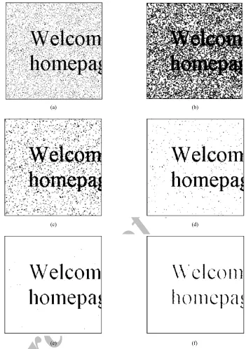
Fig. 1. (a) Original image, I₀, (b) noisy image, I, (c) resulting grayscale image thresholded at each level (H) and convolution of noisy image with binary window then thresholded to give 5 output images including the erosion (t=5), dilation (t=1) and median (t=3).

III. IMPLEMENTATION VIA LINEAR OPERATIONS

Having set out the basic definition of some simple morphological and rank order filters the paper will now consider alternative methods of implementation which may be carried out via linear processing techniques.

Consider the following statement:

All rank order filters including the median and a number of the fundamental SSP (set-set processing) tasks within mathematical morphology may be implemented simultaneously for binary images via a single linear (multiply-accumulate) operation carried out between the original image, I, and the filter window, B, followed by thresholding at an appropriate level.

The convolution operator is central to all linear software and hardware image-processing systems. The convolution

) , (mn

H between an image I and window B is defined as follows:

∑ ∑

− = =−

− − =

∗

= K

K k

L

L l

l n k m I l k B B

I n m

H( , ) ( , ) ( , ) (8)

The above operator is used in edge detection, linear smoothing and sharpening.

In order to implement the morphological operators and rank order filters, the image I and the filter window, B, are convolved to produce a single image, H. Although both I and B are binary, the result of their convolution,

H, is a grayscale image with pixel values in the range, 0 to B . The image, H, will be shown to consist of a stack of all the outputs of the rank order filter ψr, for every value

of r. The required rank order filtered output image,

) (I

r

ψ , may be obtained by thresholding the image, H , at the appropriate value of r.

The convolution of the image, I, with the window, B, is equivalent, in the binary case, to an operation which counts the number of pixels within the window, B, for which I=1,andsets the corresponding pixel in image H , to this value.

∑

= ∈

− − =

∗ =

1 ) , ( ) , (

) , ( )

, (

l k B l k

l n k m I B

I n m

H (9)

Archive of SID

(a) (b)

(c) (d)

(e) (f)

Fig. 2. The example shows a text image corrupted with 10% additive impulsive noise, then filtered with every 5 point rank order filter. It can be seen that rank r=4 gives a lower MAE than the median. (a) Noisy image, (b) r=1 dilated image, MAE= 0.392, (c) r=2 MAE= 0.087, (d) r=3 median filtered, MAE= 0.012, (e) r=4, MAE= 0.008 * optimum, (f) r=5 eroded image, MAE= 0.029.

original image I .

The binary images resulting from filtering by ψ_r, i.e. the rank order, morphological and median filters are obtained by thresholding H at the appropriate level, r. The following filters may be obtained.

• Rank order filter

[

]

r = ∗

ψ (10)

• Median Filter

( )

[

]

Med_B = B+1/2 ∗ ₍₁₁₎

• Dilation

[

]

I⊕ = 1 ∗ ₍₁₂₎

• Erosion

[

]

B

I = B ∗ (13)

where Tt[N] _{is a thresholding function defined as}

 

 ≥

=

otherwise 0

if 1 ]

[N N t

Tt .

An example is shown in Fig. 1. Fig. 1(a) shows a simple original image and Fig. 1(b) shows a noise corrupted version. The objective is to filter the noisy image in order to recover the original or an image which is as close as possible to it. As can be seen in Fig. 1(c) the resulting grayscale image contains, at each level, every rank order filter including the erosion, the dilation and the median. In this simple case the median is the best filter as it recovers the original image precisely.

Fig. 2 shows a text image corrupted with 10% additive noise. It is then convolved with a 5 point window and thresholded at each level to create the various rank order

-Archive of SID

(a) (b) (c) (d)

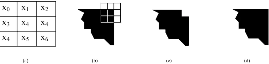
Fig. 3. (a) The labeling of the pixels within a 3×3 window, (b) location of the window at a corner pixel (there are 4 black foreground (=1) and 5 white background pixels (=0) in the window), (c) removal of the corner pixel by a standard median filter (median filter list [1, 1, 1, 1, 0, 0, 0, 0, 0] output 0, therefore the output is 0 and the corner is removed), and (d) preservation of the corner by a weighted median filtering (weighted median filter (W=3) list is [1, 1, 1, 1, 1, 1, 0, 0, 0, 0, 0], therefore the output is 1 and the corner is preserved).

filtered images. In this case the optimum filter is ψ₄ which outperforms the median, ψ₃ by a further 33% in terms of the mean absolute error (MAE).

IV. WEIGHTED MEDIAN FILTER

Another type of filter which may be implemented within the linear framework is the weighted median filter [36]-[38]. The filters described so far are essentially counting filters which give an output dependent on the number of pixels within the window which equal 1. The disadvantage of this approach, particularly for larger windows, is that it treats all pixels in the window with the same importance. In order to preserve finer image structure such as corners and straight lines it is necessary to give the pixels at some locations within the window a greater weighting.

A modification of the median filter is the weighted median (or center weighted median) in which the pixel derived from the central location of the window is included in the pixel list w times compared to the other pixels. Consider the case of a 3×3 weighted median filter. The output of this filter with weighting W and window locations labeled as in Fig. 3(a) is given by

) , , , , times repeated , , , , ( ) ( 8 7 6 5 4 4 3 2 1 0 med x x x x x W x x x x x W > < = x .

Assuming that the weighting is an odd number and again that the inputs are binary the rank ordered list will form a group of 1s followed by a group of 0s. The length of the list will be W+8 pixels so the median value will be located at position (W+9)/2 in the list. Therefore if the number of 1s in the list is greater than this value the output of the weighted median will be 1 otherwise it will be 0.

The pixel value at location x₄ is counted W times so the output of the weighted median filter will be,

     + ≥ + =

∑

( 4 ₄

med

W x Wx

W x _i i (14)

where

∑

∑

∑

= = = = ≠

+

=

i

x

x

x

In the same way as the standard median filter was applied to binary images through linear convolution and a threshold function, the weighted median filter can also be implemented in the same way. The only modification required is to set the window values to the appropriate weightings so in the case above B(0,0)=W and B(k,l)=1

for all k≠0 and l≠0. The filter output can then be written as,

( )

[

]

BW I =T W I∗B

+1/2

Med (15)

where B_W is the filter window including the weighted values and B_W is the sum of all the values in the window.

So although the weighting, W , applied in the weighted median filter refers to the number of times the center pixel is repeated, in the binary case the same output may be achieved by using, W , as a multiplicative weighting of the center pixel in the overall summation shown in (14). Therefore in the binary case, not only does the sorting operation simplify to a basic count, but also the repetition operator is replaced by a multiplicative weighting.

A. Weighting Factor Range

A problem in the application of the weighted median filter is the selection of the weighting value to be applied to the center pixel. The value of the weighting can be critical as will be seen in later examples.

B. Structural Considerations

The weighting may be chosen in order to preserve certain structures within the image. It is a simple matter to show that a basic 3×3 median filter will remove the corner pixel from a 90º angle. However by giving the center value a weighting of 3, the corner pixel will be preserved. This is demonstrated in Figs. 3(b) to 3(d). Similar variations may be introduced to preserve one pixel wide straight lines. In general the larger the weighting of the center pixel, the less change will result from filtering.

Consider the variation in window weighting for a 3×3

center weighted median:

From (14) the output of the filter W_med(x)=1 if the following inequality holds,

2 ) 9 ( 4 4 + ≥ +

∑

i . (16)

Letting W =2c+1 as W is odd, reduces (16) to

5 ) 1 2 ( 4

4+ ≥ +

+

∑

i . (17)

Archive of SID

) ( )

( ₄

med x D x

W x = ∆ (18)

where    ≠ = otherwise 0 ) ( if 1 )

(x x4 Wmed x

D (19)

and ∆ is the set difference (XOR) operator.

The differencing filter D(x) is 1 where the pixel value at the center of the window is changed by filtering. It can easily be shown that there are only four valid filter weights for the filter defined in a 3×3 window and that these are 1, 3, 5, 7. The weighting can be related directly to the number of neighboring pixels of opposite value required to cause the pixel at the center of the window to switch state. As the WMF is self dual the conditions for it to switch in either direction are the same.

For center weightings greater than, W >7 the 3×3

filter becomes the Identity filter which is neither extensive nor antiextensive.

When the weighting is W =1, the filter is identical to the standard median. For a 3×3 window it requires at least 5 neighboring pixels to possess the opposite value to the center pixel in order to cause it to switch state. For each increase in center weight, one further neighboring pixel is required to trigger a switch. This is shown in Table I.

Further generalizations to these filters may be applied by giving all pixels a weighting and by choosing ranks other than the median as the output. It is even possible with a small modification to have non-integer weightings though this is beyond the scope of this paper. The interested reader may wish to refer to [39].

V. OPTIMUM FILTER DESIGN

So far a number of non-linear filters which may be implemented through linear operators have been described. When one of these filters is employed for a specific task such as noise reduction, the problem of filter design becomes one of selecting the optimum set of parameters for the task required. Usually the optimum is the filter which minimizes some measure such as the Mean Absolute Error, MAE, between the filtered image and some ideal version. As an ideal version is required the technique uses a training set from which the optimum parameters are determined. Provided that the training set is representative then the filter found will also be optimal (or very close to optimal) for further data sets to which it is applied.

One way to determine the optimum filter ψ_opt from all possible filters is to carry out an exhaustive search by testing every filter ψ_r. This is effectively what has been carried out in Figs. 1 and 2 but it is computationally expensive for larger filters. An alternative approach is to minimize the MAE by estimating the conditional expectation of the output value [40].

For simplicity we define x=(x₀,x₁,...,x_B−1) as the observations of the noisy image, I(m,n) within the window B and y=I₀(m,n) as the corresponding pixel

3 6 5 7 7 8

>7 Not possible

value in the ideal image. The conditional expectations

) | 0 (y= x

P and P(y=1|x) are the probabilities that the filter output is 0 or 1 respectively for a given input x.

The MAE may be expressed as

∑

∑

where P(x)P(x) is the prior probability of x.

The total error consists of all the pixels where the filter output is 1 and the ideal image is 0 or vice versa. These quantities are then summed over the image.

A. Optimum Rank Order Filters

For a window of size n, each vector x can take on 2n

values, which makes finding the optimal MAE filter extremely data intensive, especially for larger windows. Suppose, however, a filter is defined based on the Hamming weight of the vector, x . Then filters are of the form φ(x), and there are only n+1 possible inputs for which it is required to determine the filter value. These filters will be called weight filters, and the optimal weight filter is given by

    < = ≥ = = 5 . 0 ) | 1 ( if , 0 5 . 0 ) | 1 ( if , 1 ) ( opt _x x x Y P Y P

φ . (21)

The filter will be correct for at least 50% of the inputs. The MAE of the optimum weight filter is summed over the cases where it gives the incorrect output:

) | 1 ( ), | 0 ( min ) ( ) ( , MAE _{0 opt}

x x x x = = × >= <

∑

The weight filter, φ_opt(x), is sub-optimal compared to the optimal of all filters defined in the window n. This is because it has been constrained to consider only the weight of the input vector, x. There is, therefore an increase in error for each input x for which the output of the φ_opt(x)

differs from the overall optimum filter.

Comparing φ_opt with ψ_r and rewriting (2), as

   ≥ = otherwise , 0 | | if , 1 ) ( r r x x

ψ (23)

then φ_opt and ψ_r depend only on the weight |x|, so they can be written as φ_opt(x) and ψ_r(x). Since φ_opt is optimal with respect to weight-based filters, its MAE cannot exceed the MAE of ψ_r, which means that rank-order filters are poorer than optimal weight filters. Indeed,

r ψ

φ_opt = if and only if P(Y =1|W)≥0.5 for W ≥r and

5 . 0 ) | 1 (Y = W <

Archive of SID

(a) (b)

(c) (d)

Fig. 4. (a) The noisy and ideal image observations, (b) the probability estimates with the optimum rank order filter ropt=6, (c) the noisy image filtered at 6

=

r , and (d) the noisy image filtered at median r=5.

j i j y

P i y

P( =1| x = )≥ ( =1|x = ) for > . (24) Then φ_opt =ψ_ropt, where r_opt =minimum value of r for which P(y=1|x =r)>0.5.

The weight-monotonic property states loosely that the more black pixels in the observation window, the more likely it is that the ideal pixel at the window center is black. The model is not unreasonable for ideal images in which the micro-geometry is somewhat random and the noise is white and symmetric. Simulation show that these assumptions hold for restoration type problems where the noisy and ideal images have similar pixel values, but they do not hold for inverted or edge detected images. Rank order filters would not be applicable for the latter type of images.

The difficulty in this general approach to filter design is in obtaining a good estimate of the conditional and prior probabilities P(y=1|x) and P(x) respectively for each value of x. In restricting the class of functions to that

corresponding to rank order filters, a smaller set of conditional and prior probabilities P(y=1|x) and P(x)

must be estimated. This is carried out through the collection of observations of a representative training sequence.

An example of optimum filter design within a 3×3

window, is shown in Fig. 4. Fig. 4(a) shows the observations for a pixel in the ideal image, where N(y=0) and N(y=1) indicates the number of times the ideal value corresponded to either 0 or 1 for the various values of x in the noisy image. Fig. 4(b) shows the estimates of the prior and conditional probability calculated from these values. For this image the optimum rank order filter is where r_opt =6, as this is the minimum value of r for which P(y=1| x)>0.5. This gives an MAE of 0.0068, which equates to 444 pixels in error. This figure is equivalent to summing the minimum value of either

=

y

Archive of SID

(a) (b)

(c) (d)

(e)

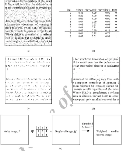
Fig. 5. (a) The detail in noisy image containing very thin text, (b) the probability estimates gives the optimum weighted median, (c) the filtered image using the standard median filter, (d) the filtered image using the weighted median filter with W=5 (equivalent to xc′ =7), and (e) the implementation of weighted median filter. The noisy image I is linearly convolved with the window, B shown to produce the grayscale image H, which is then thresholded at level 7 to give the weighted median filter with W=5.

If the median (i.e. r=5) were used instead of using the optimum filter then the increase in MAE would be 0.00036. This Fig. which is equivalent to a further 24 pixels in error can be obtained directly from the table of observations, as 308 pixels would be in error for x =5

instead of 284 pixels, i.e. N(y=0|x =5) instead of

) 5 | 1 (y= x =

N .

B. Optimum Weighted Median Filter Design

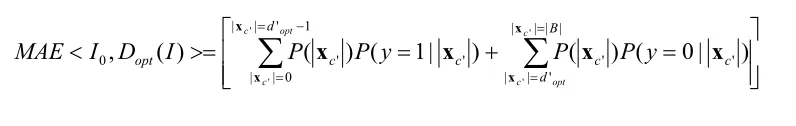
The design of the optimum weighted median filter within a window B, reduces to the problem of determining the pixel weighting, W , for which the MAE is a minimum. As explained earlier this problem may be placed in the context of a difference filter, D(I).

For simplicity let d =D(I). Then P(d =1| x_c′) is the

probability that x_c will switch value when x_c′ of its

neighbors have the opposite value. Similarly

) | 0 (d _c

P = x ′ is the probability that xc will remain unchanged under the same conditions. The prior probability |xc'| is given by P(xc′).

Assuming that the weight-monotonic property holds, then the probability that a pixel will switch state increases monotonically with the number of neighbors it has with the opposite value.

The optimum differencing filter D_opt(I) is determined by d_opt′ the minimum value of x_c′ for which

5 . 0 ) | 1 (d= _c′ >

P x .

Similarly the total MAE

Archive of SID

















=

+

=

>=

<

∑

∑

= − = = | | | | ' | | ' ' 1 ' | | 0 | | ' ' 0 ' ' ' '

)

|

0

(

)

(

)

|

1

(

)

(

)

(

,

y

P

P

y

P

P

I

D

I

MAE

x

x

x

x

_________________________________

The conditional and prior probabilities may be estimated from observations of representative training images. Fig. 5(a) shows an image containing very thin text. The probability estimates in Fig. 5(b) show that a value of

7

opt′ =

d gives the optimum weighted median. This corresponds to a weight of W =5. In contrast applying the standard median results in the destruction of most of the text as shown in Fig. 5(c). The result of applying the optimum weighted filter is shown in Fig. 5(d) and it can be seen that most of the text is preserved. The filters with weights on either side of the optimum, i.e. W =3 and 7 give very poor results, which suggests that the selection of the optimum weight is critical.

Fig. 5(e) shows an overview of the algorithm used to implement the optimum weighted median filter. It can been seen that the sorting stage has been replaced by a linear convolution with mask B(0,0)=5 and B(k,l)=1 for all

0

≠

k or l≠0. This is followed by thresholding at

7 2 / ) 9

(W+ = . C. Error Estimates

Clearly in practical situations the ideal image is not available. Where the process is repeatable such as transmission error it is possible to transmit a number of test images to build the training set. In other cases it is necessary to model the noise in some way. A vitally important part of these methods lies in using the correct size of training set. Where a training set is too small an additional error known as the precision error is introduced. This quantity is a random function as it depends on the training set.

For a basic 3×3 filtering window, the 9 input variables means that there are 229 ≈10154 different logic functions which may be implemented. For larger windows the number of functions grows rapidly. The training set required to estimate the conditional probabilities in order to determine the optimum function out of all these combinations may be impossibly large. In this work the number of functions has been reduced to the set of functions which implement rank order, morphological and weighted median functions. The optimum parameters for these filters have been obtained from a training set of a few test images with negligible estimation error. A full discussion of the problems of estimation error in this type work is given in [41].

VI. CONCLUSIONS

Many researchers and engineers reject morphological and other non-linear image processing because of the need to introduce additional hardware or software functions to their system. This work has shown how a useful subset of non-linear operations may be implemented using linear image processing tools to obtain median, rank,

morphological and weighted median filters. Analysis and examples have been included to show the reader how to estimate the optimum filter parameters for these various types of filter. The work in this paper has been limited to binary image processing but it is also possible to use a similar framework for the implementation of grayscale functions. This will be the subject of a future paper.

ACKNOWLEDGEMENT

The author would like to thank Professor E. R. Dougherty of University of Texas A&M, for his helpful comments on an earlier draft of this manuscript.

REFERENCES

[1] J. Serra, Image Analysis and Mathematical Morphology, Academic Press, London, 1982.

[2] G. Matheron, Random Sets and Integral Geometry, John-Wiley, New-York, 1975.

[3] P. Maragos and R. Schafer, "Morphological filters - part I: their set theoretic analysis and relations to linear shift-invariant filters," IEEE Trans. on Acoustics, Speech, and Signal Processing, vol. 35, no. 8, pp. 1153-1169, Aug. 1987.

[4] A. C. Bovik, T. S. Huang, and D. C. Jr. Munson, "Nonlinear filtering using linear combinations of order statistics," in Proc. IEEE Int. Conf. on Acoustics, Speech and Signal Processing, pp. 2067-2070, Paris, May 1982.

[5] A. C. Bovik, T. S. Huang, and D. C. Jr. Munson, "A generalization of median filtering using linear combinations of order statistics,"

IEEE Trans. Acoust., Speech, Signal Processing, vol. 31, no. 6, pp. 1342-1350, Dec. 1983.

[6] A. Gasteratos, Specialized Hardware Structures for Morphological Image Processing, http://argo.lira.dist.unige.it/antonis/morphology/ morphological_hardware%20_files/iv.htm.

[7] I. Andreadis, A. Gasteratos, and P. Tsalides, "An ASIC for fast gray-scale dilation," Microprocessors and Microsystems, vol. 20, no. 2, pp. 89-95, Apr. 1996.

[8] R. Lin and E. K. Wong, "Logic gate implementation for gray-scale morphology," Pattern Recognition Letters, vol. 13, no. 7, pp. 481-487, Jul. 1992.

[9] C. C. Pu and F. Y. Shih, "Threshold decomposition of gray-scale soft morphology into binary soft morphology," CVGIP-Graphical

Models and Image Processing, vol. 57, no. 6, pp. 522-526,

Nov. 1995.

[10] F. Y. Shih, and O. R. Mitchell, "Threshold decomposition of gray-scale morphology into binary morphology, IEEE Trans. on Pattern

Analysis and Machine Intelligence, vol. 11, no. 1, pp. 31-42,

Jan. 1989.

[11] C. Chen and D. L. Yang, "Realisation of morphological operations,"

IEE Proceedings: Circuits Devices and Systems, vol. 142, no. 6, pp. 364-368, Dec. 1995.

[12] I. Diamantaras and S. Y. Kung, "A linear systolic array for real-time morphological image processing," Journal of VLSI Signal Processing, vol. 17, no. 1, pp. 43-55, Sep. 1997.

[13] A. Gasteratos, I. Andreadis, and P. Tsalides, "Improvement of the majority gate algorithm for gray-scale dilation/erosion," Electronics Letters, vol. 32, no. 9, pp. 806-807, Apr. 1996.

[14] A. Gasteratos, I. Andreadis, and P. Tsalides, "Extension and very large scale integration implementation of the majority-gate algorithm for gray-scale morphological operations," Optical Engineering, vol. 36, no. 3, pp. 857-861, Mar. 1997.

Archive of SID

vol. 4, no. 3, pp. 387-391, Mar. 1995.

[18] L. Abbott, R. M. Haralick, and X. Zhuang, "Pipeline architectures for morphologic image analysis," Machine Vision and Applications, vol. 1, no. 1, pp. 23-40, Spring 1988.

[19] I. Diamantaras, K. H. Zimerman, and S. Y. Kung, "Integrated fast implementation of mathematical morphology operations in image processing", in Proc. IEEE International Symposium on Circuits and Systems, pp. 1442-1445, New Orleans, May 1990.

[20] A. Gasteratos and I. Andreadis, "Non-linear image processing in hardware," Pattern Recognition, vol. 33, no. 6, pp. 1013-1021, Jun. 2000.

[21] S. Kojima and T. Miyakawa, "One-dimensional processing architecture for gray-scale morphology," Systems and Computers in Japan, vol. 27, no. 12, pp. 1-9, Nov. 1996.

[22] F. Robin, M. Renaudin, G. Privat, and N. v.d. Bossche, "Functionally asynchronous array processor for morphological filtering of greyscale images," IEE Proceedings: Computers and Digital Techniques, vol. 143, no. 5, pp. 273-281, Sep. 1996.

[23] S. Siskos, S. Vlassis, and I. Pitas, "Analog implementation of fast min-max filtering," IEEE Trans. on Circuits and Systems II: Analog and Digital Signal Processing, vol. 45, no. 7, pp. 913-918, Jul. 1998. [24] K. Urahama and T. Nagao, "Direct analog rank filtering," IEEE

Trans. on Circuits and Systems I: Fundamental Theory and Applications, vol. 42, no. 7, pp. 385-388, Jul. 1995.

[25] S. Vlassis, S. Siskos, and I. Pitas, "Analog implementation of an order statistics filter", in Proc. 9th Mediterranean Electrotechnical Conference, MELECON’98, pp. 649-653, May 1998.

[26] E. C. Botha and D. P. Casasent, "Applications of optical morphological transformations," Optical Engineering, vol. 28, no. 5, pp. 501-505, May 1989.

[27] D. Casasent, "General-purpose optical pattern recognition image processors," Proceedings of the IEEE, vol. 82, no. 11, pp. 1724-1734, Nov. 1994.

[28] N. Woolfries, S. Marshall, and P. Lysaght, "Non-linear image processing on field programmable gate arrays," Noblesse Workshop

on Non-linear Model based Image Analysis, NMBIA98, Glasgow,

1998.

[29] K. Chen, "Bit-serial realizations of a class of nonlinear filters based on positive Boolean functions," IEEE Trans. on Circuits and Systems, vol. 36, no. 6, pp. 785-794, Jun. 1989.

[30] A. Gasteratos, I. Andreadis, and P. Tsalides, "Realization of rank-order filters based on majority gate," Pattern Recognition, vol. 30, no. 9, pp. 1571-1576, Sep. 1997.

[31] D. S. Bloomberg, "Implementation efficiency of binary morphology," in Proc.Int. Symp. for Mathematical Morphology VI, ISMM2002, pp 209-218, Sydney, Australia, Apr. 2002.

relationship to median filters," IEEE Trans. Acoust., Speech, Signal Processing, vol. 32, no. 1, pp. 145-153, Feb. 1984.

[36] L. Yin, R. Yang, M. Gabbouj, and Y. Neuvo, "Weighted median filters: a tutorial", IEEE Trans on Circuits and Systems-II: Analog

and Digital Signal Processing, vol. 43, no. 3, pp. 157-192,

Mar. 1996.

[37] D. R. K. Brownrigg, "The weighted median filter", Commun. ACM, vol. 27, no. 8, pp. 807-818, Aug. 1984.

[38] B. I., Justusson, "Median filtering: statistical properties", Topics in Applied Physics, Two-Dimensional Digital Signal Processing II, T. Huang, Ed., Springer-Verlag, Berlin, vol. 43, pp. 161-196, 1981. [39] J. Astola and P. Kuosmanen, Fundamentals of Non-linear Digital

Filtering, CRC Press, New York, 1997.

[40] E. R. Dougherty and J. Barrera, "Logical image operators" in E. R. Dougherty and J. T. Astola, Non-linear Filters for Image Processing, pp. 1-58, SPIE, Washington, 1999,

[41] E. R. Dougherty and R. Loce, "Precision of morphological-representation estimators for translation invariant binary filters: Increasing and non increasing," Signal Processing, vol. 40, no. 2-3, pp. 129-145, Nov. 1994.

Stephen Marshall was born in Sunderland, England in 1958. He received a first class honors degree in Electrical and Electronic Engineering from the University of Nottingham in 1979 and a PhD in Image Processing from University of Strathclyde in 1989. In between he worked at Plessey Office Systems, Nottingham, University of Paisley and the University of Rhode Island, USA. He is currently a Reader in the Department of Electronic and Electrical Engineering at the University of Strathclyde. His interests are non-linear image processing techniques, including mathematical morphology, genetic algorithms and novel image coding. He has published over 100 conference and journal papers on these topics; these include SPIE Journal of Electronic Imaging, SIAM, IEEE ICASSP and EUSIPCO. He has also been a reviewer for these and other journals and conferences.

Dr Marshall has participated in the NAT and Noblesse European Projects in non-linear image processing techniques. He has chaired various workshops and special sessions and been a guest editor for SPIE Electronic Imaging Journal. He edited the proceedings of the NMBIA workshop on Non-linear Model Based Image Coding in Glasgow, 1998 of which he was General Chairman.