Resolving degeneracy in diffusion MRI biophysical model parameter estimation using double diffusion encoding

Magn Reson Med. 2019;82:395–410. wileyonlinelibrary.com/journal/mrm

|

Resolving degeneracy in diffusion MRI biophysical model

parameter estimation using double diffusion encoding

Santiago Coelho

_|

_{Jose M. Pozo}

_|

_{Sune N. Jespersen}

_|

_{Derek K. Jones}

_|

Alejandro F. Frangi

1_{Centre for Computational Imaging & Simulation Technologies in Biomedicine (CISTIB) and Leeds Institute for Cardiac and Metabolic Medicine}

(LICAMM), School of Computing & School of Medicine, University of Leeds, Leeds, United Kingdom

2_{CISTIB, Electronic and Electrical Engineering Department, The University of Sheffield, Sheffield, United Kingdom}

3_{Center of Functionally Integrative Neuroscience (CFIN) and MINDLab, Department of Clinical Medicine, Aarhus University, Aarhus, Denmark} 4_{Department of Physics and Astronomy, Aarhus University, Aarhus, Denmark}

5_{Cardiff University Brain Research Imaging Centre (CUBRIC), Cardiff University, Cardiff, United Kingdom} 6_{School of Psychology, Australian Catholic University, Melbourne, Australia}

This is an open access article under the terms of the Creative Commons Attribution License, which permits use, distribution and reproduction in any medium, provided the original work is properly cited.

© 2019 The Authors. Magnetic Resonance in Medicine published by Wiley Periodicals, Inc. on behalf of International Society for Magnetic Resonance in Medicine

Correspondence

Santiago Coelho, CISTIB, School of Computing, University of Leeds, EC Stoner Building, Rm 6.01, Woodhouse Lane, Leeds LS2 9JT, United Kingdom. Email: [email protected] Twitter: @santicoelho

Purpose: Biophysical tissue models are increasingly used in the interpretation of dif-fusion MRI (dMRI) data, with the potential to provide specific biomarkers of brain microstructural changes. However, it has been shown recently that, in the general Standard Model, parameter estimation from dMRI data is ill‐conditioned even when very high b‐values are applied. We analyze this issue for the Neurite Orientation Dispersion and Density Imaging with Diffusivity Assessment (NODDIDA) model and demonstrate that its extension from single diffusion encoding (SDE) to double diffu-sion encoding (DDE) resolves the ill‐posedness for intermediate diffudiffu-sion weightings, producing an increase in accuracy and precision of the parameter estimation.

Methods: We analyze theoretically the cumulant expansion up to fourth order in b of SDE and DDE signals. Additionally, we perform in silico experiments to compare SDE and DDE capabilities under similar noise conditions.

Results: We prove analytically that DDE provides invariant information non‐acces-sible from SDE, which makes the NODDIDA parameter estimation injective. The in silico experiments show that DDE reduces the bias and mean square error of the estimation along the whole feasible region of 5D model parameter space. Conclusions: DDE adds additional information for estimating the model parameters, unexplored by SDE. We show, as an example, that this is sufficient to solve the pre-viously reported degeneracies in the NODDIDA model parameter estimation.

1

|

INTRODUCTION

Diffusion MRI (dMRI) has been established as an invalu-able tool for characterizing brain microstructure in vivo

and non‐invasively. Diffusion weighted images (DWIs) are sensitive to the random displacement of water mole-cules within a voxel,1 _{probing tissue on scales}

consider-ably lower than image resolution.2 _{Diffusion MRI provides}

the aggregate signal from the distribution of components within a voxel. By measuring across multiple diffusion ori-entations and weightings, information about the underlying tissue architecture can be unravelled. The ability to detect small alterations in brain tissue is a key factor when de-veloping biomarkers for early stages of neurodegenerative diseases.3 _{Various approaches to derive information from}

Diffusion Weighted Images (DWI) have been proposed in the literature.4–8 _{Most direct approaches, such as Diffusion}

Tensor Imaging (DTI),4 _{are just aimed at describing the}

main MRI signal characteristics (signal representations,9_).

However, the quest for specific information on tissue microstructural integrity inspired the development of biophysical tissue models.10–13 _{By assuming certain}

char-acteristics for the tissue, such as the type of constituents, their geometry and physical properties, these models may allow the extraction of more specific microstructural in-formation than signal representations, as long as these assumptions are at least approximately satisfied by the tissue. Nevertheless, the validity of these results relies on how accurate the model is for the tissue under study. The widely used Neurite Orientation Dispersion and Density Imaging (NODDI)14 _{model fixes the diffusivity values of}

the compartments present in the voxel to specific values. NODDI’s assumptions have been shown to be incompat-ible with data from spherical tensor encoding (STE) in Lampinen et al15 _{and it has been argued to introduce bias}

in the estimation of the remaining model parameters.16

To overcome this limitation, Jelescu et al17 _{extended the}

model by adding the diffusivities to the estimation rou-tine, and removing the CSF compartment. They dubbed it NODDIDA (NODDI with Diffusivity Assessment). While this approach eliminated some flawed assump-tions made by NODDI, this led to multiple possible solu-tions that describe the signal equally well. This reflects that the estimation problem is ill‐posed or, at least, ill‐ conditioned, and is usually stated as the existence of de-generated model parameter sets. Recent work by Novikov et al showed that this degeneracy is intrinsic to the so‐called Standard Model (SM),18 _{of which NODDIDA is a special}

case. They show that choosing the correct solution is chal-lenging even with the use of high b‐value data, although Jespersen et al19 _{obtained stable estimations in ex‐vivo brain}

tissue using extremely high b‐values (15 ms/μm2). Reisert

et al20 _{proposed a supervised machine learning approach}

trained with the expected value of the Bayesian posterior, which, by definition, disregards the possible multimodality of the distribution. Furthermore, it was trained on simu-lated data with the prior assumption of similar traces for the intra‐ and extra‐axonal diffusivities.

Most of the dMRI techniques have been developed for an acquisition performed within a Single Diffusion Encoding (SDE) framework. Since Stejskal and Tanner developed the Pulsed Gradient Spin Echo (PGSE) sequence,21 _{there have}

been many works aimed at maximizing the information that can be obtained from a dMRI experiment by exploring dif-ferent acquisition protocols.22,23 _{One of the many}

modifica-tions proposed to the magnetic gradient waveforms involves the addition of multiple gradient pairs. Particularly, a scheme that has lately gained popularity is termed double diffusion encoding (DDE),24 _{first proposed by Cory et al.}25 _{The term}

DDE refers to any sequence consisting of two consecutive diffusion encodings. It has been shown that DDE, as well as other multiple encoding schemes, has the potential to provide new information that is not immediately accessible with SDE.26 _{Many groups focused on developing methods}

for extracting microstructural information based on this scheme.27–30 _{Jespersen et al}31 _{showed that in the}

low‐diffu-sion‐weighting limit, the information extracted from single and multiple diffusion encodings is the same. A recently developed dMRI framework based on q‐space trajectory encoding (i.e. multidimensional diffusion encoding) was proposed to probe tissue in ways not accessible by SDE.32

For tissues comprised of multiple Gaussian compartments (MGCs) any q‐space trajectory is equivalent to a second order b‐tensor, which generalizes the concept of b‐value. In such systems SDE and DDE are fully specified by b‐ten-sors, with one and two non‐zero eigenvalues, respectively, and are also called linear tensor encoding (LTE) and planar tensor encoding (PTE), in case of DDE with perpendicular directions. Lampinen et al15 _{have analyzed the advantages}

of a multidimensional encoding over SDE NODDI. They proved that extending the acquisition increases the accuracy in quantifying microscopic anisotropy. However, it has not been fully explored, from the point of view of fitting a bio-physical model to noisy measurements, if single or multiple encodings can provide us with more precise model parameter estimates (cf.29,30_{). Recently, the advantages of combining}

K E Y W O R D S

linear with planar or spherical tensor encoding to address the degeneracy and increase the precision of parameter estima-tion have been investigated33–35 _{in both in silico and/or in} vivo experiments. Their results show that the estimation pre-cision is increased by the addition of these orthogonal mea-surements. However, a theoretical background of why this happens is still missing.

This paper extends NODDIDA to a DDE scheme and as-sesses the accuracy of estimators based on SDE and DDE measurements. This extension adds more degrees of freedom to the data acquisition (i.e. two diffusion encoding periods must be chosen). We hypothesized that DDE acquisition pro-tocols containing both parallel and perpendicular direction pairs might outperform SDE protocols in informing biophys-ical models. We investigated analytbiophys-ically the different infor-mation provided by DDE and SDE in terms of their fourth order cumulant expansions. We examine the ill‐posed nature of the parameter estimation from SDE and present a theoreti-cal explanation of why DDE resolves the degeneracy (except for the completely isotropic case κ = 0) without requiring extremely high diffusion weightings (e.g. b>4 ms∕μm2).

Additionally, we generated in silico dMRI measurements for acquisitions with different DDE configurations from a wide range of model parameter values covering the biologically feasible region of the 5D parameter space. Under similar experimental conditions, higher accuracy and precision is obtained for DDE combining parallel and perpendicular di-rection pairs, outperforming SDE in most scenarios.

2

_|

THEORY

2.1

_|

Biophysical model assumptions

A general assumption among multi‐compartment models rep-resenting tissue microstructure is that water exchange between compartments is negligible for typical experimental time scales. The total signal is the weighted contribution from each compartment. The two‐compartment model dubbed Standard Model is the most general version of the typical models used for diffusion in neural tissue (see Ref.36_{). The stick}

compart-ment (sometimes referred as intra‐neurite) represents axons, which are expected to be the main contributors to the restricted diffusion signal, and, possibly, dendrites and glial processes.19

The inclusion of dendrites and glial processes is open to dis-cussion36 _{and implies the assumption that in certain regimes}

(depending on e.g. diffusion time) they have similar diffusiv-ity and T₂ relaxation properties and directional distribution, a

question which still has not been fully addressed (see partial discussion in Lampinen et al37_{). Sticks are zero‐radius}

cylin-ders and model fibers in which diffusion is assumed to occur only along the fiber’s main direction as it was first proposed for water in neurites in Jespersen et al.13 _{Later, Nilsson et al}38

showed theoretically that typical axonal diameters cannot be

resolved with SDE and gradient amplitudes available on clini-cal scanners and thus, are indistinguishable from sticks. This was also confirmed experimentally in Veraart et al.39 _The

sec-ond compartment represents the extra‐neurite space where dif-fusion is hindered and is modeled as Gaussian anisotropic19

(zeppelin compartment). A fiber segment is defined as the local bundle of aligned sticks with the extra‐neurite space surrounding them. Voxels are composed of a large number of fiber segments. The SM consists of the fiber segment signal model (i.e. kernel) with the diffusivities and water fraction as free parameters, together with a general fiber orientation dis-tribution function (ODF), which could be represented by its spherical harmonics decomposition. One limitation of this model is that each fascicle within a voxel is assumed to have identical diffusion properties, leading to identical microstruc-tural parameters.

Some other works consider a third compartment that rep-resents the contribution from stationary water.11,40 _However,

recent works41 _{have concluded that the signal arising from}

this compartment can be neglected in most structures for the diffusion times used in the clinic and should only be con-sidered in the cerebellum.42 _{Additionally, in its original}

ver-sion, NODDI included an isotropic diffusion compartment to account for the presence of cerebrospinal fluid (CSF). This compartment was removed from NODDIDA for the sake of simplicity.17

Considering a general fiber ODF involves a large set of parameters, which can hinder their unambiguous estimation from the dMRI signal. The NODDIDA model,17 _is

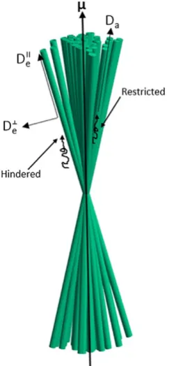
essen-tially the SM with the constraint that the fiber ODF must be a Watson spherical distribution (u)̂ =f(û|𝝁̂,𝜅), with

con-centration parameter κ and main direction 𝝁̂ (see Figure 1). This cylindrically symmetric ODF is usually considered a sufficiently good and parsimonious model,43 _{especially for}

white matter regions without crossing fibers. Although being a simplified version of SM, NODDIDA still presents some degeneracy problems. Thus, in this work, we focus our anal-ysis on the NODIDDA model.

2.2

_|

NODDIDA model with SDE

For a general SM, the signal from a SDE experiment, where the diffusion weighting b (i.e. b‐value) is applied in the diffu-sion encoding direction n̂ =[n_x,n_y,n_z]t, is given by the

con-volution over the unit sphere18

where

(1)

S_SDE(b,n)̂ =S₀

�𝕊2

(u)̂ (b,n̂⋅_{u)d̂ S}

̂

u,

(2) (b,n̂⋅_û)=fexp[_−bD

a(n̂⋅û)2 ]

+(1−f) exp[−bD⟂

e−bΔe(n̂⋅û)2 ]

is the response signal (kernel) from a fiber segment oriented along direction û. Here, f is the (mainly) T₂‐weighted stick

volume fraction, D_a the intra‐neurite axial diffusivity, and

Δ_e=D‖_e−D⟂

e, with D

‖

e, D⟂e the extra‐neurite diffusivities

parallel and perpendicular to the fiber‐segment axis.36 _These

scalar kernel parameters (f, D_a, D‖_e, and D⟂

e) provide

impor-tant tissue microstructural information, and have shown potential clinical relevance as they are sensitive to specific disease processes such as demyelination, axonal loss or inflammation.44–46

It has been recently shown that the parameter estimation is challenging under normal experimental conditions.17 _There

are two issues here. The first one is that fitting these mod-els to noisy measurements is generally a non‐convex opti-mization problem, potentially having several local minima of the objective function, requiring appropriate optimization algorithms. However, the existence of multiple local minima opens the door to a second, more serious, issue: the objec-tive function can present multiple minima with equal or very similar values. In the presence of noise these minima are per-turbed, making unstable which one becomes the global min-imum. Jelescu et al17 _{evidenced this ill‐posedness issue for}

clinically feasible dMRI acquisitions in two particular cases. They showed that the estimated parameters from a collection of independently simulated dMRI measurements follow a bi‐modal distribution, despite being simulated from a single ground truth, and the presence of practically indistinguish-able spurious minima in the objective function.

2.3

_|

Parameter estimation from SDE: An

ill‐posed problem

A recent work by Novikov et al18 _{analyzed in detail this}

in-verse problem for the unconstrained SM by reparametrizing it into its rotational invariants. They concluded that without any constraints on the ODF shape, it was not possible to estimate the kernel parameters with an acquisition sensitive up to order

(b2). However, in this work we are interested in studying

NODDIDA, where the ODF is given by a Watson distribution. For intermediate diffusion weightings (i.e. b<2.5 ms∕μm2)

the dMRI signal is accurately represented by its 4th‐order

cu-mulant expansion47 _{(sensitive up to (b}2₎ contributions). For

SDE this expansion can be written as8

where S₀ =S(b=0) is the unweighted signal, D and W

are the diffusion and kurtosis tensors, respectively, with ̄

D=tr(D), as defined in Hansen et al48 and Einstein’s

sum-mation convention is implied. Let us consider a voxel with fibers oriented according to a Watson ODF. Following an analogous procedure as in Novikov et al18 we can expand the signal S(b,n)̂ in Equation 1 up to order (b2₎ according to

Equation 3. This gives a mapping between the biophysical parameter (BP) space and the diffusion kurtosis (DK) space, removing the dependence with the acquisition settings and simplifying the analysis of whether different sets of model parameters produce the same signal profile.

Due to the axial symmetry of the Watson distribution, the corresponding diffusion and kurtosis tensors can be ex-pressed in terms of the projection, 𝜉=n̂⋅_𝝁̂, of the gradient

direction to the main direction 𝝁̂ Jespersen et al49,1 :

where h2(𝜉,𝜅)= 1 3+

2

3p2P2(𝜉) and h4(𝜉,𝜅)=

1 5+

4

7p2P2(𝜉)+ 8 35p4P4(𝜉)

are defined as in Jespersen et al49_P

2(𝜉) and P4(𝜉) are the

sec-ond and fourth order Legendre polynomials, and p₂, p₄ the

non‐zero second and fourth order coefficients of the spherical harmonics expansion of the Watson distribution:

where F denotes the Dawson function.50 Using these equa-tions, we can derive the relations between the BP and DK parameters that fully describe this axially symmetric environ-ment, as done in Hansen et al51 _{for fully aligned fibers, but}

here for an arbitrary value of κ:

(3)

log (S(b,n̂)∕S₀)≈ −bn_in_jD_ij+1₆b2_D̄2_n

injnkn𝓁Wijk𝓁

= −bD(n̂)+1₆b2_D̄2_W(n̂),

(4) D(𝜉)=(fD_a+(1−f )Δe)h2(𝜉,𝜅)+(1−f )D⟂e,W(𝜉)D̄

2

=3[(fD2

a+(1−f )Δ 2 e )

h₄(𝜉,𝜅)+2(1−f )Δ_eD⟂

eh2(𝜉,𝜅) +(1−f )D⟂2

e −D(𝜉) 2]_,

(5)

p₂=1

4

�

3

√

𝜅F(√𝜅)−2− 3

𝜅 �

,

p₄= 1

32𝜅2

�

105+12𝜅(5+𝜅)+5 √

𝜅(2𝜅−21) F(√𝜅)

�

, FIGURE 1 Diagram of the two compartments present in the

where _D̄ _=(2D

⟂+D‖)∕3. Taking the limit for κ→∞ we

re-cover the system of equations for parallel fibers presented in Hansen et al51 _{(Equation 12).}

In Hansen et al48 _{the equivalent to the system in Equation 6}

is solved reaching two alternative equations for κ, _±(𝜅)=0,

each giving possible solutions. This suggested that, in gen-eral, there should be two solutions, one for each branch. However, this is not always the case, as illustrated in Table 1. We derive here an alternative expression of the solution in one equation only. First, Equation 6 can be reparametrized as:

After this substitution, Equation 6 can be expressed as a linear system of five equations for the 5 unknowns α, β, γ, δ

and ε, decoupled into two independent smaller systems:

Observe that the coefficients of matrices L and M depend on κ. We will ignore for the moment that the five unknowns are not independent. The solution is unique as long as matrices L and M are invertible. This is the case when κ ≠ 0, since detL=p₂ and detM= −1

2p2p4. In the

limit of a fully isotropic medium (κ = 0) the system has only two independent equations, not allowing the recover-ing of the kernel parameters without additional informa-tion. By solving the two systems in Equation 8 we find expressions for α, β, γ, δ and ε that only depend on κ and the DK parameters (see Appendix A for solution). Those vari-ables are actually defined from only four kernel parameters (Equation 7), resulting in the coupling equation

(6)

D_‖= (fD_a+(1−f )Δe)h2(1,𝜅)+(1−f )D⟂e,

D_⟂= (fD_a+(1−f )Δe)h2(0,𝜅)+(1−f )D⟂e,

1 3W‖D̄

2_+D2

‖= (fD2a+(1−f )Δ2e)h4(1,𝜅)+2(1−f )ΔeD⟂eh2(1,𝜅)+(1−f )D⟂e2,

1 3W⟂D̄

2_+D2 ⟂= (fD

2

a+(1−f )Δ 2

e)h4(0,𝜅)+2(1−f )ΔeD⟂eh2(0,𝜅)+(1−f )D⟂e2,

5W̄D̄2 8 −

W⟂D̄

2 4 −

W‖D̄2 24 +

(D⟂+D‖)2 4 = (fD

2

a+(1−f )Δ 2 e)h4(

1

√

2,𝜅) +2(1−f )ΔeD ⟂ eh2(

1

√

2,𝜅) +(1−f )D ⟂2 e ,

(7) 𝛼=f Da+(1−f )Δe,𝛽 =(1−f )D⟂e,𝛾 =f D

2

a+(1−f )Δ 2 e, 𝛿=(1−f )Δ_eD⟂

e, 𝜖 =(1−f )D⟂ 2 e . (8) � D_‖ D_⟂ � = �

h2(1,𝜅) 1 h2(0,𝜅) 1

� � 𝛼 𝛽 � =L � 𝛼 𝛽 � , ⎡ ⎢ ⎢ ⎢ ⎣ 1 3W‖D̄

2_+D2

‖

1 3W⟂D̄

2_+D2 ⟂ 5W̄D̄2

8 −

W_⟂D̄2

4 −

W_‖D̄2

24 + (D_⟂+D_‖)2

4 ⎤ ⎥ ⎥ ⎥ ⎦ = ⎡ ⎢ ⎢ ⎢ ⎣

h4(1,𝜅) 2h2(1,𝜅) 1 h4(0,𝜅) 2h2(0,𝜅) 1 h4(

1

√

2,𝜅) 2h2( 1

√

2,𝜅) 1 ⎤ ⎥ ⎥ ⎥ ⎦ ⎡ ⎢ ⎢ ⎢ ⎣ 𝛾 𝛿 𝜖 ⎤ ⎥ ⎥ ⎥ ⎦ =M ⎡ ⎢ ⎢ ⎢ ⎣ 𝛾 𝛿 𝜖 ⎤ ⎥ ⎥ ⎥ ⎦ . (9) 𝛾(𝜖−𝛽2)=𝛼2𝜖+𝛿2−2𝛼𝛽𝛿.

TABLE 1 Illustration of sets of biophysical (BP) parameter values resulting in the same diffusion–kurtosis (DK) parameters

DK parameters Branch BP parameters C new invariants

[D‖,D_⟂,W‖,W_⟂,W̄] [f,Da,D

‖

e,D⟂e,𝜿] ζ1 ζ2

[1.503, 0.195, 1.456, 0.291, 0.926] + [0.730, 2.000, 1.000, 0.300, 8.000] −0.006 0.210

− [0.607, 1.287, 2.191, 0.318, 11.49] 0.023 0.053

[1.557, 1.048, 0.396, 0.708, 0.330] + [0.250, 2.370, 1.300, 1.390, 50.00] 0.349 0.624

− — —

[0.457, 0.408, 2.901, 2.702, 2.770] + [0.879, 1.320, 1.401, −0.232, 0.265] −0.190 0.022

− [0.870, 0.950, 2.000, 0.720, 0.360] −0.023 0.014

− [0.549, 0.182, 1.071, 0.766, 1.414] 0.154 −0.002

− [0.510, 0.076, 0.931, 0.794, 3.187] 0.161 −0.005

[1.560, 1.256, 0.423, 0.540, 0.506] + — —

− [0.240, 1.450, 2.100, 1.400, 2.330] 0.237 0.125

− [0.189, 0.668, 1.887, 1.489, 5.442] 0.325 0.057

By plugging the expressions for α, β, γ, δ and ε as functions of κ into Equation 9, we obtain a nonlinear equation for κ

with potentially multiple solutions. Each solution for κ gives a single solution for α, β, γ, δ and ε, which in turn, gives a single solution for the kernel parameters:

Thus, the number of solutions to Equation 9 corresponds to the number of BP parameter sets that have the same DK pa-rameters. Table 1 presents cases with up to four solutions. We computed the number of solutions for 10k random points in the BP parameter space. Most present two solutions (70.2%), some only one (29.3%), and only a small proportion have four solutions (0.5%). This gives rise to the previously dis-cussed degeneracy in model parameter estimation from noisy measurements.17 _{In contrast with the claim in Hansen et al}51

even in the extreme case of parallel fibers leaving only four unknowns, the five equations in Equation 6 are independent. This is possible due to the nonlinear nature of the system. If κ

is known and not zero (including the limiting case κ → ∞ of parallel fibers), the full‐system is invertible as long as f is not 0 or 1, and D⟂

e is not null. In that case, each point in the DK

parameter space (signal profile) corresponds to a single set of BP parameters. However, this is not the case for an arbitrary unknown κ. Here, the full‐system has five independent equa-tions with five unknowns, but, depending on the parameter values, it can have only one or multiple solutions. This latter case makes the inverse mapping an ill‐posed problem.

Using very high b‐values might be considered an option to solve this problem, as it will add higher order terms in Equation 3. However, it is still challenging due to very low associated signal‐to‐noise ratio (SNR) and is also unfeasible in most clin-ical scanners, although bespoke systems with ultra‐strong gra-dients may provide leverage in this regard.52 _{Another solution}

that does not require powerful gradients is to seek for indepen-dent measurements providing new information.

2.4

_|

Model extension to DDE

DDE adds an extra dimension to the dMRI acquisition, unex-plored by SDE experiments. For a general multidimensional acquisition,32,53 _{due to the assumption of impermeable}

com-partments, within each of which the diffusion displacement profile is assumed to be Gaussian, the signal can be written as:

with the kernel

for b = tr(B). The b‐tensor of a DDE acquisition is

B=b₁n̂₁⊗ ̂n₁+b₂n̂₂⊗ ̂n₂, defined from the pair of gradient

directions, n̂₁, n̂₂, and their individual diffusion weightings, b₁, b₂. It has in general two non‐zero eigenvalues, viz. PTE. In

con-trast, the SDE’s b‐tensor, B=bn̂ ⊗ ̂n, has only one non‐zero

eigenvalue, viz. LTE. Hence, for this model a SDE acquisition is a subset of the DDE acquisitions (SDE=DDE_‖ ⊂DDE),

for which n̂₁=n̂₂ (parallel direction pair).

2.5

_|

DDE information gain

DDE can, in principle, provide independent complemen-tary information. This could transform the inverse map-ping of recovering BP parameters from diffusion‐weighted measurements into a well‐posed problem. The fourth order cumulant expansion for the dMRI signal arising from a DDE experiment is

Here, C is the second cumulant tensor of the dMRI signal expansion in terms of the b‐tensor and satisfies minor and major symmetries:

but it is not totally symmetric. Its totally symmetric part is proportional to the kurtosis tensor:

For MGCs or DDE with long mixing times,31_{D and C can be}

written as

where f_𝛼 and D(_ij𝛼) denote the fraction and diffusion tensor of

compartment α, including in this summation the integral over the unit sphere with the ODF (cf. Equation 1). This motivated naming C as the diffusion tensor covariance.31,32 _Our

defini-tion of C coincides with the one in Westin et al32 _{and for long}

mixing times it is also proportional to the Z tensor (C=Z∕(4Δ2₎), earlier introduced in Jespersen.31 The Z

ten-sor is defined more generally, i.e. not restricted to MGCs, as a cumulant of the DDE signal.

In the case of a Watson ODF, W and C are transversely isotropic fourth order tensors, i.e. they have cylindrical sym-metry. Hence, instead of having 15 and 21 independent com-ponents they only have three and five, respectively. We can write both tensors as a function of coordinate independent tensor forms (for full derivation see Appendix B), like it is done for W in Hansen et al51 _{(Equation 6):}

(10) f=1−𝛽

2

𝜖 ,Da= 𝛼𝜖−𝛽𝛿

𝜖−𝛽2 ,Δe= 𝛿 𝛽,D

⟂

e= 𝜖 𝛽.

(11)

S_NODDIDA(B)=S₀

�𝕊2

(u)̂ (B,u)d̂ S_û,

(12)

(B,u)̂ =fexp[ −D_aB_iju_iu_j] +(1−f) exp[ −bD⟂_e− Δ_eB_iju_iu_j],

(13)

log (S∕S₀)= −B_ijD_ij+ 1

2BijBk𝓁Cijk𝓁

= −(b1n1in1j+b2n2in2j)Dij +D̄2

6(b 2

1n1in1jn1kn1𝓁+b₂2n2in2jn2kn2𝓁)Wijk𝓁

+b₁b₂n_1in_1jn_2kn₂𝓁Cijk𝓁.

(14)

C_ijk𝓁 =Cjik𝓁 =Cij𝓁k =Ck𝓁ij,

(15) ̄

D2W_ijk𝓁 =3C₍ijk𝓁₎ =Cijk𝓁 +Ci𝓁jk+Cik𝓁j.

(16) Dij=⟨Dij⟩=

∑

𝛼

f𝛼D

(𝛼)

ij ,

Cijk𝓁= �

(D_ij−⟨D_ij⟩)(D_k𝓁−⟨D_k𝓁⟩) �

=∑ 𝛼

f𝛼D

(𝛼)

ij D

(𝛼)

where C was written separating its fully symmetric part from the remaining part,54 _and

where 𝛿_ij is the Kronecker delta and 𝝁̂ the Watson distribution main direction. Equation 17 shows explicitly that C contains two extra degrees of freedom independent of W. Observe that the fully symmetric part of R and J vanishes, so that the in-formation encoded in 𝜁₁ and 𝜁₂ is not accessible from a SDE experiment.28 _{We can isolate the new non‐symmetric}

compo-nents by the antisymmetrization

Considering a coordinate frame with the z‐axis parallel to the fibers main direction 𝝁̂, we can identify

Similarly to Equation 6 we can relate the elements of C to the biophysical parameters like it was done for W. For the SM, including NODDIDA, D and C are given by

where

For NODDIDA we get h₂(𝜉,𝜅)=H_ij(2)n_in_j and h₄(𝜉,𝜅)=H_ijk(4)_𝓁n_in_jn_kn𝓁, with 𝜉 =𝝁̂⋅n̂. The cross‐terms of C

present new information not accessible from SDE. This makes the DDE signal able to resolve the degeneracy. To make this explicit, we can write the components isolated in Equation 20 in the adapted coordinate frame in terms of BP parameters:

Those two equations are independent to the ones in Equation 6, adding complementary information to the mapping between DK and BP spaces (see last column in Table 1). Using the same variables defined in Equation 7 we get

These two equations enlarge the system in Equation 8. Following the derivation in Appendix C, we demonstrate that they determine a single solution for κ:

since the left‐hand side is a strictly monotone increasing function on κ. This agrees with recent work by Cotaar et al,55 who showed that combining different b‐tensor shapes can determine robustly fiber dispersion. Observe that the cases f = 0 or f = 1 reflect only an apparent degeneracy, as the different sets of parameters represent the same physical model. In contrast, the case of κ = 0 presents a proper degeneracy of the model due to lack of information, where different model instances have identi-cal D and C tensors.

3

_|

METHODS

3.1

_|

Signal generation

All synthetic measurements were generated from substrates composed of 1 μm diameter cylinders to simultaneously as-sess our stick approximation. We found this difference was below the noise level. We computed the signal attenuation in the cylinder’s perpendicular plane with the Gaussian phase approximation for both SDE56 _{and DDE.}30

Since there is no closed analytical solution for the integral on the sphere in Equation 11, we computed the spherical con-volution using Lebedev’s quadrature57_:

where wi are the quadrature weights of each grid point ûi

across the unit sphere. For all configurations of SDE and DDE we used 1,202 quadrature points, which guarantee an exact result up to a 59th order spherical harmonics

decom-position of the ODF. No practical differences were found between the results from our SDE implementation and the analytic summation for SDE in Zhang et al.43

Finally, Rician noise was added to the synthetic signals, normalizing it to obtain a SNR = 50 for the b₀ measurements,

like in Jelescu et al.17

(17) W=𝜔₁P+𝜔₂Q+𝜔₃I and C= 1

3 ̄

D2W+𝜁₁R+𝜁₂J,

(18)

Pijk𝓁=𝜇i𝜇j𝜇k𝜇𝓁,

Qijk𝓁=

1 6

(

𝜇i𝜇j𝛿k𝓁+𝜇k𝜇𝓁𝛿ij+𝜇i𝜇k𝛿j𝓁+𝜇j𝜇k𝛿i𝓁+𝜇i𝜇𝓁𝛿jk+𝜇j𝜇𝓁𝛿ik )

,

I_ijk𝓁=

1 3

(

𝛿_ij𝛿_k𝓁+𝛿ik𝛿j𝓁+𝛿i𝓁𝛿jk )

,

Rijk𝓁=

1 2

(

𝜇i𝜇j𝛿k𝓁+𝜇k𝜇𝓁𝛿ij )

−1

4

(

𝜇i𝜇k𝛿j𝓁+𝜇j𝜇k𝛿i𝓁+𝜇i𝜇𝓁𝛿jk+𝜇j𝜇𝓁𝛿ik )

,

J_ijk𝓁=𝛿ij𝛿k𝓁−

1 2

(

𝛿_ik𝛿_j𝓁+𝛿i𝓁𝛿jk )

,

(19)

C_ijk𝓁−Cikj𝓁 =𝜁₁(Rijk𝓁−Rikj𝓁)+𝜁2(Jijk𝓁−Jikj𝓁).

(20)

Cxxyy−Cxyxy= 3

2𝜁2 and Cxxzz−Cxzxz−Cxxyy+Cxyxy= 3 4𝜁1.

(21)

D_ij= [f D_a+(1−f)Δe]H (2)

ij +(1−f)D⟂e𝛿ij,

C_ijk𝓁= [f D2_a +(1−f)Δ2_e]H

(4)

ijk𝓁

+(1−f)D⟂

eΔe (

𝛿ijH

(2)

k𝓁 +𝛿k𝓁H

(2)

ij

)

+(1−f)D⟂2

e 𝛿ij𝛿k𝓁−DijDk𝓁,

(22)

H_ij(2)=_�

𝕊2

(û)u_iu_jdS_û and H(4)

ijk𝓁=� 𝕊2

(û)u_iu_ju_ku𝓁dSû.

(23) 3

2𝜁2=Cxxyy−Cxyxy =(1−f)

�

D⟂

eΔe �

H(2)_xx +H_yy(2)

� +D⟂

e 2�

−DxxDyy

=(1−f)�2D⟂

eΔeh2(0,𝜅)+D⟂e 2�

−D2

⟂,

3

4𝜁1=Cxxzz−Cxzxz−Cxxyy+Cxyxy =(1−f)D⟂

eΔe �

H(2)

zz −H

(2)

yy

�

−D_xx(D_zz−D_yy) =(1−f)D⟂

eΔe(h2(1,𝜅)−h2(0,𝜅)) −D⟂(D‖−D⟂).

(24) 2h₂(0,𝜅)𝛿+𝜖 = 3

2𝜁2+D 2

⟂ and

(h2(1,𝜅)−h2(0,𝜅))𝛿= 3

4𝜁1 +D⟂(D‖−D⟂).

(25)

h₄(1,𝜅)

h₄(0,𝜅) = 1 3W‖D̄

2₋3

2(𝜁1 +𝜁2)+(D‖−D⟂) 2

1 3W⟂

̄

D2₋3

2𝜁2

(26)

∫𝕊2

f (û)dS_û≈∑ i

3.2

_|

Parameter estimation algorithm

Parameter estimation was based on a nonlinear least squares estimator. This was justified due to the relatively high SNR considered for the experiments, where Rician noise can be approximated as Gaussian.58 _{We used the Trust Region}

Reflective algorithm implemented in the MATLAB (R2016a, MathWorks, Natick, Massachusetts) optimization toolbox. The objective cost function was

where N is the total number of measurements, B_i

in-dicates the b‐tensor used in the i‐th measurement and

𝜽=[f,D_a,D‖_e,D⟂

e,𝜅] is a vector containing the model

param-eters. The main direction of the fibers, 𝝁̂, and S₀ were fitted

independently in a first stage through a DTI fitting like in Jelescu et al.17 _{For all configurations, this optimization}

pro-cedure was repeated using 30 independent random initializa-tions for the model parameters to avoid local minima of the five‐dimensional cost function. The local solution with the lowest residue was the global optimum.

3.3

_|

SDE and DDE tested configurations

Five encoding configurations were considered: DDE₆₀₊₀, DDE₄₀+20, DDE30+30, DDE20+40, and DDE0+60, with

pro-gressively increasing proportions of perpendicular direction pairs, b, with respect to parallel direction pairs, a, denoted as DDEa+b. Observe that DDE60+0 is equivalent to SDE if

MGCs are assumed. We compared the SDE protocol used in Jelescu et al17 _{against different DDE acquisitions with}

the same number of measurements that can be measured in a similar experimental time. The SDE measurement proto-col had two shells with b‐values of 1 and 2 ms∕μm2 with

30 directions each.17 _{These directions were generated using}

the Sparse and Optimal Acquisition (SOA) scheme.59 DDE configurations were also divided in two shells with the same b‐values as above and both directions in each pair had equal individual diffusion weightings, b₁=b₂= 1

2b. Thus,

per-pendicular direction pairs define axially symmetric planar b‐tensors, uniquely defined by their normal vector. We gen-erated homogeneously distributed normal vectors using the same algorithm used for the SDE directions. The DDE₃₀₊₃₀

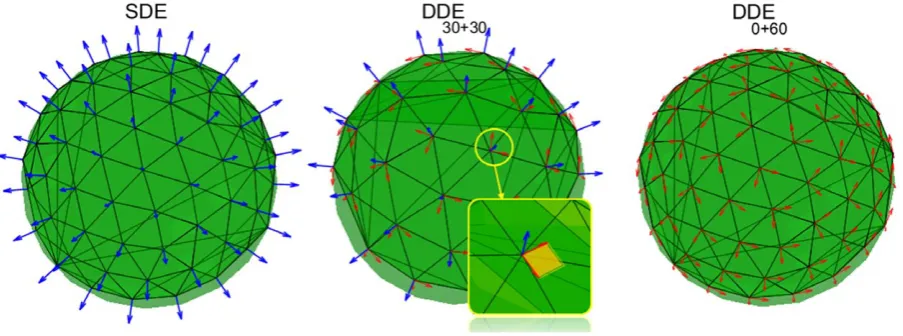
acquisition had 30 parallel direction pairs and 30 perpen-dicular direction pairs with normal vectors coinciding with the parallel pairs33 (see middle diagram in Figure 2). The DDE₀₊₆₀ protocol had only perpendicular directions

pairs (right diagram in Figure 2). Configuration DDE₄₀+20

had two parallel per each perpendicular directions pair, and DDE₂₀+40 two perpendicular per each parallel

direc-tions pair. All acquisidirec-tions had five non diffusion‐weighted measurements (i.e. b₀ measurements).

3.4

_|

Experiments

We performed two in silico experiments to assess whether the addition of DDE measurements can enhance the pa-rameter estimation in the presence of typical noise in the measurements.

In the first experiment, we considered two possible instances of NODDIDA parameter values for a voxel in the posterior limb of the internal capsule (PLIC) taken from Jelescu et al17 _(see

Table 2), for which SDE estimates showed a bimodal distribu-tion. We explored in detail whether DDE solves the degeneracy between these particular cases. Only SDE and DDE₃₀₊₃₀

acqui-sition configurations were considered for this experiment. Two thousand and five hundred independent realizations of Rician noise were added to the synthetic SDE and DDE signals.

The second experiment aims to compare the ac-curacy and precision provided by SDE and the differ-ent DDE configurations extensively along the feasible region of the full five‐dimensional (5D) space of param-eters (diffusivities between 0 and 3μm2_∕ms, fraction

be-tween 0 and 1, and κ positive). This allows exploring whether there are subregions presenting different behav-iors. A 5D grid was generated by all the combinations of

f = [0.1, 0.3, 0.5, 0.7, 0.9], Da=[0.3,0.8,1.3,1.8,2.3]μm2∕ms, D‖_e =[0.8, 1.3, 1.8]μm2_∕ms, _D⟂

e =[0.5, 1, 1.5]μm

2_∕ms, and κ = [0.84, 2.58, 4.75, 9.27, 15.53, 33.70]. The fraction and the diffusivities were selected from a uniform discreti-zation of the expected range, and κ values were chosen such that the mean‐squared‐cosine corresponding angle, ⟨cos2_𝜑⟩=c

2=⟨(û⋅𝝁̂)2⟩= (2

√

𝜅F(√𝜅))−1−(2𝜅)−1, was

𝜑=[50◦ , 40◦

, 30◦ , 20◦

, 15◦ , 10◦

] (c₂ = [0.41, 0.59, 0.75, 0.88, 0.93, 0.97]). We generated 50 independent Rician noise realizations (SNR = 50) for the measurements of each com-bination of the parameters for the five configurations.

4

_|

RESULTS

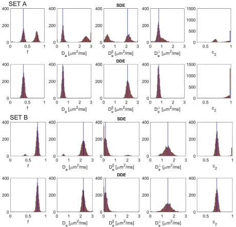
Histograms of the estimated model parameters from the first experiment (Figure 3) show an increase in the accuracy and precision of the estimates with the DDE scheme. The bimodal distribution of the estimated parameters is evident with the SDE acquisition, confirming that it is not possi-ble to differentiate true and spurious minima. This effect is removed when using the DDE sequence.

We analyzed the shapes of the SDE and DDE ob-jective functions from the synthetic measurements of SET A (sum of squared differences: F_A(𝜽)). To

facil-itate the visualization of these 5D functions, we per-formed a 1D cut through a straight line joining the true and spurious minima of SDE. This was parametrized with the scalar variable t: 𝜽=t𝜽_spur+(1−t)𝜽_true;t∈[0, 1],

where 𝜽_true=[0.38, 0.5, 2.1, 0.74, 64] and

(27)

F(𝜽)=

N

∑

i

𝜽_spur=[0.78, 2.67, 0.32, 0.85, 3.65], with diffusivities

ex-pressed in μm2_∕ms. Figure 4 shows the behavior of _F A(𝜽)

along this cut as a function of t. It can be observed that al-though the DDE objective function is still bimodal, the spu-rious and true minima have significantly different absolute values (due to the contribution of the tensor C to the DDE signal). This enables us to distinguish both peaks in condi-tions where SDE cannot (i.e. b_max=2 ms∕μm2). Adding

more directions to the SDE acquisition would not help to dif-ferentiate the peaks, as even in the noiseless case these two sets produce the same signal. Only by increasing the SDE diffusion weighting the spurious minimum could be differen-tiated from the true one.

For each point in the 5D grid of parameters, the Root Mean Square Error (RMSE, for definition see for instance60₎

of each parameter has been computed from 50 independent noise realizations. The distributions of RMSE of the param-eter estimates from this second experiment are displayed in Figure 5 with violin plots (similar to box plots but showing also estimated probability density61_{). The summary statistics}

of the RMSE distributions are shown in Table 3. On aver-age, DDE₄₀₊₂₀ and DDE₃₀₊₃₀ are the most accurate

config-urations for estimating all parameters. This suggests that the

incorporation of even a small proportion of DDE measure-ments can remove the degeneracy, leading to an increase in accuracy and precision.

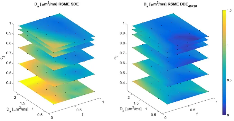
To compare the performance of SDE and DDE in different regions of the parameter space, we projected the 5D RMSE map onto different 3D sub‐spaces. Figures 6 and 7 show two different 3D projections, over (D‖_e, D⟂_e,c₂(𝜅)) and

over (f,D_a,c₂(𝜅)), of the RMSE of f and D_a, respectively. The

highest improvement of DDE with respect to SDE is asso-ciated with low c₂ values, i.e. high orientation dispersion.

Additionally, for highly aligned voxels the performances of both schemes becomes similar.

5

_|

DISCUSSION

Our work shows that modifying the diffusion MRI pulse sequence can mitigate the degeneracy on NODDIDA’s pa-rameter estimation. Our proposal circumvents the need of presetting diffusivities to a priori values as in NODDI. We showed that estimating the NODDIDA model through SDE is generally an ill‐posed problem. Depending on the specific combination of model parameters, multiple parameter sets may produce the same signal profile. We show analytically that DDE makes parameter estimation well‐posed, and illus-trate for a particular model instance the better behaved cost function obtained with DDE. In silico experiments over a wide range of model parameter combinations confirmed that extending the acquisition to DDE makes the inverse prob-lem well‐posed and solves the degeneracy in the parameter estimation. Combining DDE parallel (i.e. LTE) and perpen-dicular (i.e. PTE) direction pairs not only provides more sta-ble parameter estimates but also increases their accuracy and precision.

FIGURE 2 Diagram of different measurement protocols (SDE, DDE30+30, and DDE0+60). Only SDE and DDE30+30 were used in experiment 1, while they all were used in experiment 2. Blue colors denote the SDE directions or DDE parallel direction pairs. DDE perpendicular direction pairs are in red

TABLE 2 Ground truth for experiment 1

Model parameter SET A SET B

f 0.38 0.77

Da[μm2∕ms] 0.50 2.23

D‖_e[μm2_∕ms] 2.10 0.16

D⟂ e[μm

2_∕ms] 0.74 1.48

In Section 2, we showed that considering a noise‐free scenario, in the case of fibers following a Watson ODF with known (nonzero) concentration parameter κ (including the case of parallel fibers), the inverse problem of recovering biophysical parameters from SDE measurements is well‐ posed. This is not the case for arbitrary unknown concen-tration κ, where Jelescu et al17 _{first showed experimentally}

that the parameter estimation from SDE with intermediate b‐values was degenerated. This was analyzed in Jespersen et al49 _{showing that there were two nonlinear equations}

providing possible solutions. We demonstrated that in the absence of noise the number of BP parameter sets that de-scribe the signal equally well up to (b2₎ can be either 1, 2,

or 4. In contrast, we showed analytically that the C tensor includes non‐symmetric independent components that are accessible by DDE, but not by SDE, allowing the complete inverse mapping between the cumulant signal representation and BP parameter space. Consistently, the first experiment showed that in both of the PLIC synthetic voxels, DDE leads to more accurate and precise parameter estimations. This is clearly seen when analyzing the optimization cost‐function which shows that although DDE also presents multiple local minima, the global minimum is substantially deeper, unlike SDE, thus it can be picked in typical noise levels. However, two points in the 5D model parameter space are insufficient to draw more general conclusions. Therefore, the second

experiment swept the parameter space extensively using a regular grid. Mean results (see Table 3) showed the min-imum RMSE for an acquisition consisting of both linear and planar b‐tensors, suggesting that the optimal combina-tion for the scenario considered is between DDE₄₀₊₂₀ and DDE₃₀+30 configurations.

Increasing the total number of measurements and SNR will have a larger impact in enhancing DDE parameter esti-mation than with SDE, since the bimodality present in SDE implies a non‐zero lower bound for the achievable MSE even without noise. Results from34 _{show that the addition}

of STE data also leads to an increase in the precision of

D_a and f in in vivo experiments. In our synthetic

experi-ments the addition of PTE data reduces the RMSE in all the parameter estimates (to a lesser extent in f and D⟂

e).

Recently, Dhital et al35 _{showed through in silico}

experi-ments that incorporating PTE data to LTE data enabled

us to discriminate spurious solutions in the cost‐function. This latter result is explained by our theoretical analysis in Section 5 where we derive the independent equations pro-vided by DDE that make the inverse problem well‐posed. While finalizing this paper, a preprint62 _{appeared, reaching}

similar conclusions.

Biophysical models are promising for extracting micro-structure‐specific information but care must be taken when applying them in dMRI. Some assumptions are more mean-ingful than others and hence their impact on parameter esti-mation must be assessed.9 _{Invalid assumptions in the model}

will likely produce bias in the resulting microstructural in-formation, which is epistemic and thus such biases cannot be removed simply by removing the degeneracy. Releasing the diffusivities in the typical two‐compartment model elimi-nates an invalid assumption, reduces possible biases in the es-timated parameters, and provides extra information amenable

FIGURE 4 Plots of F_A(𝜽(t)) for different values of t ∈ [−0.05,1.05], with 𝜽(t)=t𝜽_spur+(1−t)𝜽_true. Black curves show F_A values for noise‐free

SDE and DDE₃₀+30 acquisitions. The colored curves show 30 independent realizations of FA for SNR = 50

FIGURE 5 Violin plots of the RMSE for all model parameters for all voxels in the 5D grid (a total of 5×5×3×3×6 = 1,350). Black dots denote the mean and red lines the median. The RMSE for each voxel was computed by repeating the estimation on 50 independent noise realizations of the measurements for each voxel

TABLE 3 Mean and standard deviation of the RMSE over the whole grid for each acquisition protocol and each of the estimated parameters

RMSE (μ; σ) f Da[𝛍m2∕ms] D

‖

e[𝛍m

2_{∕ms] D}⟂

e[𝛍m

2_{∕ms] c} 2=f(𝜿)

SDE 0.14; 0.12 0.74; 0.43 0.51; 0.33 0.33; 0.27 0.13; 0.08

DDE40+20 0.10; 0.10 0.39; 0.30 0.41; 0.31 0.29; 0.25 0.08; 0.07

DDE30+30 0.11; 0.10 0.39; 0.29 0.42; 0.30 0.30; 0.25 0.08; 0.07

DDE20+40 0.11; 0.10 0.40; 0.30 0.43; 0.31 0.31; 0.25 0.08 ; 0.07

to be used as a biomarker of microstructural integrity and sensitive to specific disease processes.44,45,63 _{In this work, we}

have focused on analyzing the estimability of the model under different acquisition settings. The validation against comple-mentary real data is an independent problem. Both should be addressed further to bring biophysical models to the clinic.

Jespersen et al19 _{showed the estimation of the SM was}

stable and without degeneracy when using extremely high b‐ values (15 ms∕μm2) on ex vivo data. Recent work by Novikov

et al18 _{studied the unconstrained SM and concluded that}

if high b‐values are unfeasible then orthogonal measure-ments might be an alternative to uniquely relate the kernel

FIGURE 6 RMSE of f, for SDE and DDE₄₀₊₂₀ acquisition protocols. This 3D plot shows the projection over D‖e, D⟂e, and c2 of all the RMSE in the 5D grid. This projection was made by computing the square root of the quadratic mean of the errors in the remaining 2 dimensions (Eproj,ijk=

�∑

𝓁

∑

mEijk2𝓁m∕(N𝓁Nm)). Black dots denote the actual points in the grid, linear interpolation was used to generate the color figures

FIGURE 7 RMSE of D_a, for SDE and DDE₄₀+20 acquisition protocols. This 3D plot shows the projection over f, Da, and c2 of all the RMSE in the 5D grid. This projection was made by computing the square root of the quadratic mean of the errors in the remaining 2 dimensions (Eproj,ijk=

�∑

𝓁

∑

parameters to the signal. Veraart et al extended the SM to acquisitions with varying echo time (TE).64 _{This latter work}

goes in a similar direction to our work here, i.e. adding extra dimensions to the experiment and changing the objective function to avoid ill‐posedness. However, measuring multi-ple directions while varying the TE implies increasing the acquisition time and TE, affecting the SNR. However, this approach can be combined with DDE leading to a DDE acquisition with multiple TEs. Recently, Lampinen et al15

showed that by acquiring data with linear and spherical ten-sor encodings the accuracy in estimating the microstructural anisotropy was increased compared to that derived from NODDI’s parameters. Additionally, Dhital et al41 _measured

the intracellular diffusivity using isotropic encoding. These two works point in a similar direction than ours, i.e. extend-ing the acquisition to combine different shapes of b‐tensors to maximize accuracy and precision. Future work will study the generalization of the model to a multidimensional diffusion acquisition, since the C tensor can be fully sampled using different combinations of b‐tensor shapes, not only by LTE + PTE. Also, a detailed analysis of the impact of noise will be performed, further assessing the practical identifiability of the model parameters.

This work’s aim was to demonstrate that it is possible to solve the intrinsic degeneracy of the SM with a Watson fODF using DDE. Although a cylindrically symmetric fODF might be insufficient to model crossing fibers, it may provide a reasonable approximation in the spinal cord and certain other white matter fiber bundles,65 _{or in highly}

dispersed tissues like gray matter. Work by Tariq et al has extended the initial NODDI model to a Bingham ODF.66

Additionally, Novikov et al18 _{proposed the unconstrained}

SM with ODF to be described by a series of spherical harmonics. We plan to extend the analysis in this paper to general ODFs. The extension of biophysical models to multidimensional dMRI acquisitions32 _{should be further}

explored. The comparisons made in this work between SDE and DDE protocols do not consider the optimization of the diffusion directions in DDE, just taking four arbitrary cho-sen DDE protocols extrapolated from an optimized SDE. We expect that further optimization of the DDE acquisition protocol may also lead to larger improvements. Finally, the largest errors in the parameter estimates occur for κ → 0. This might mean that for highly dispersed tissue (i.e. grey matter) many measurements might be needed to accurately estimate model parameters.

6

_|

CONCLUSIONS

The potential increase in sensitivity and specificity in detecting brain microstructural changes is a major driv-ing force for developdriv-ing biophysical models. However,

non‐linear parameter estimation of these models is not nec-essarily well‐posed and can lead to unreliable parameter values. In this work, we not only extended the NODDIDA biophysical model from SDE to DDE schemes, but also demonstrated theoretically the advantages this latter ap-proach has. We illustrated how DDE resolves the degen-eracy issue intrinsic to this model estimation from SDE. We prove theoretically that DDE provides complementary information that makes the parameter estimation well‐ posed. Additionally, this extension leads to an increase in the accuracy and precision in the model parameter esti-mates in the presence of noise. The combination of paral-lel and perpendicular measurements for optimal parameter estimation as function of SNR and measurement time re-mains to be investigated. Our approach does not require high diffusion weightings to make the inverse problem well‐posed and it can be further developed for the uncon-strained SM.

ACKNOWLEDGMENTS

This work has been supported by the OCEAN project (EP/ M006328/1) and MedIAN Network (EP/N026993/1) both funded by the Engineering and Physical Sciences Research Council (EPSRC) and the European Commission FP7 Project VPH‐DARE@IT (FP7‐ICT‐2011‐9‐601055). DKJ is supported by a Wellcome Trust Investigator Award (096646/Z/11/Z) and a Wellcome Trust Strategic Award (104943/Z/14/Z).

NOTE

1_{These equations are presented in Ref. [49] (Equation 9). However, in their}

expression, Δ_e incorrectly appears squared also in the second term of the equation for W(𝜉)D̄2. This was a typing error.

REFERENCES

1. Callaghan PT. Physics of Diffusion. In: Jones DK, editor. Diffusion MRI: Theory, Methods and Applications. Oxford: Oxford University Press; 2010:45–56.

2. Kiselev VG. Fundamentals of diffusion MRI physics. NMR Biomed. 2017;30:1–18.

3. Assaf Y. Can we use diffusion MRI as a bio‐marker of neurodegen-erative processes? BioEssays. 2008;30:1235–1245.

4. Basser PJ, Mattiello J, LeBihan D. Estimation of the Effective Self‐Diffusion Tensor from the NMR Spin Echo. J Magn Reson. 1994;103:247–254.

5. Assaf Y, Cohen Y. Structural information in neuronal tissue as re-vealed by q‐space diffusion NMR spectroscopy of metabolites in bovine optic nerve. NMR Biomed. 1999;12:335–344.

8. Jensen JH, Helpern JA, Ramani A, Lu H, Kaczynski K. Diffusional Kurtosis imaging: the quantification of non‐Gaussian water diffu-sion by means of magnetic resonance imaging. Magn Reson Med. 2005;53:1432–1440.

9. Novikov DS, Kiselev VG, Jespersen SN. On modeling. Magn Reson Med. 2018;79:3172–3193.

10. Gelderen PV, Despres D, Zijl PCMV, Moonen CTW. Evaluation of restricted diffusion in cylinders phosphocreatine in rabbit leg muscle. J Magn Reson Ser B. 1994;103:255–260.

11. Stanisz GJ, Szafer A, Wright GA, Henkelman RM. An analytical model of restricted diffusion in bovine optic nerve. Magn Reson Med. 1997;37:103–111.

12. Assaf Y, Blumenfeld‐Katzir T, Yovel Y, Basser PJ. New model-ing and experimental framework to characterize hindered and re-stricted water diffusion in brain white matter. Magn Reson Med. 2004;52:965–978.

13. Jespersen SN, Kroenke CD, Østergaard L, Ackerman JJH, Yablonskiy DA. Modeling dendrite density from magnetic reso-nance diffusion measurements. NeuroImage. 2007;34:1473–1486. 14. Zhang H, Schneider T, Wheeler‐Kingshott CA, Alexander DC.

NODDI: practical in vivo neurite orientation dispersion and density imaging of the human brain. NeuroImage. 2012;61:1000–1016. 15. Lampinen B, Szczepankiewicz F, Mårtensson J, van Westen

D, Sundgren PC, Nilsson M. Neurite density imaging versus imaging of microscopic anisotropy in diffusion MRI: a model comparison using spherical tensor encoding. NeuroImage. 2017;147:517–531.

16. Hutchinson EB, Avram AV, Irfanoglu MO, et al. Analysis of the effects of noise, DWI sampling, and value of assumed parameters in diffusion MRI models. Magn Reson Med. 2017;78:1767–1780. 17. Jelescu IO, Veraart J, Fieremans E, Novikov DS. Degeneracy in

model parameter estimation for multi‐compartmental diffusion in neuronal tissue. NMR Biomed. 2016;29:33–47.

18. Novikov DS, Veraart J, Jelescu IO, Fieremans E. Rotationally‐in-variant mapping of scalar and orientational metrics of neuronal mi-crostructure with diffusion MRI. NeuroImage. 2018;174:518–538. 19. Jespersen SN, Bjarkam CR, Nyengaard JR, et al. Neurite density

from magnetic resonance diffusion measurements at ultrahigh field: comparison with light microscopy and electron microscopy. NeuroImage. 2010;49:205–216.

20. Reisert M, Kellner E, Dhital B, Hennig J, Kiselev VG. Disentangling micro from mesostructure by diffusion MRI: a Bayesian approach. NeuroImage. 2017;147:964–975.

21. Stejskal EO, Tanner TE. Spin diffusion measurements: spin echoes in the presence of a time‐dependent field gradient. J Chem Phys. 1965;42:288–292.

22. Jones DK. The effect of gradient sampling schemes on measures derived from diffusion tensor MRI: a Monte Carlo study. Magn Reson Med. 2004;51:807–815.

23. Alexander DC. A general framework for experiment design in dif-fusion MRI and its application in measuring direct tissue‐micro-structure features. Magn Reson Med. 2008;60:439–448.

24. Shemesh N, Jespersen SN, Alexander DC, et al. Conventions and nomenclature for double diffusion encoding NMR and MRI. Magn Reson Med. 2015;75:82–87.

25. Cory DG, Garroway AN, Miller JB. Applications of spin transport as a probe of local geometry. Polymer Preprints 1990;31:149. 26. Mitra PP. Multiple wave‐vector extensions of the NMR pulsed‐

field‐gradient spin‐echo diffusion measurement. Phys Rev B. 1995;51:15074–15078.

27. Özarslan E, Shemesh N, Basser PJ. A general framework to quan-tify the effect of restricted diffusion on the NMR signal with appli-cations to double pulsed field gradient NMR experiments. J Chem Phys. 2009;130:104702/1–104702/9.

28. Jespersen SN, Lundell H, Sønderby CK, Dyrby TB. Orientationally invariant metrics of apparent compartment eccentricity from dou-ble pulsed field gradient diffusion experiments. NMR Biomed. 2013;26:1647–1662.

29. Benjamini D, Komlosh ME, Basser PJ, Nevo U. Nonparametric pore size distribution using d‐PFG: comparison to s‐PFG and mi-gration to MRI. J Magn Reson. 2014;246:36–45.

30. Ianuş A, Drobnjak I, Alexander DC. Model‐based estimation of microscopic anisotropy using diffusion MRI: a simulation study. NMR Biomed. 2016;29:672–685.

31. Jespersen SN. Equivalence of double and single wave vector diffusion contrast at low diffusion weighting. NMR Biomed. 2011;25:813–818.

32. Westin CF, Knutsson H, Pasternak O, et  al. q‐space trajectory imaging for multidimensional diffusion MRI of the human brain. NeuroImage. 2016;135:345–362.

33. Coelho S, Beltrachini L, Pozo JM, Frangi AF. Double diffusion encoding vs single diffusion encoding in parameter estimation of biophysical models in diffusion‐weighted MRI. In Proceedings of the 25th Annual Meeting of ISMRM, Honolulu, HI, 2017:3383. 34. Fieremans E, Veraart J, Ades‐Aron B, Szczepankiewicz F, Nilsson

M, Novikov DS. Effects of combining linear with spherical ten-sor encoding on estimating brain microstructural parameters. In Proceedings of the 26th Annual Meeting of ISMRM, Paris, France, 2018:0254.

35. Dhital B, Reisert M, Kellner E, Kiselev VG. Diffusion Weighting with linear and planar encoding solves degeneracy in parameter estimation. In Proceedings of the 26th Annual Meeting of ISMRM, Paris, France, 2018:5239.

36. Novikov DS, Fieremans E, Jespersen SN, Kiselev VG. Quantifying brain microstructure with diffusion MRI: theory and parameter estimation. NMR Biomed. 2018:e3998.

37. Lampinen B, Szczepankiewicz F, Novén M, et al. Searching for the neurite density with diffusion MRI: challenges for biophysical modeling. 2018; arXiv:1806.02731.

38. Nilsson M, Lasicˇ S, Drobnjak I, Topgaard D, Westin CF. Resolution limit of cylinder diameter estimation by diffusion MRI: the impact of gradient waveform and orientation dispersion. NMR Biomed. 30:e3711.

39. Veraart J, Fieremans E, Novikov DS. On the scaling behavior of water diffusion in human brain white matter. NeuroImage. 2018;185:379–387.

40. Alexander DC, Hubbard PL, Hall MG, et al. Orientationally in-variant indices of axon diameter and density from diffusion MRI. NeuroImage. 2010;52:1374–1389.

41. Dhital B, Kellner E, Kiselev VG, Reisert M. The absence of restricted water pool in brain white matter. NeuroImage. 2018;182:398‐406.

42. Tax C, Szczepankiewicz F, Nilsson M, Jones D. The Dot... where-fore art thou? Search for the isotropic restricted diffusion com-partment in the brain with spherical tensor encoding and strong gradients. In Proceedings of the 26th Annual Meeting of ISMRM, Paris, France, 2018:0253.