White Rose Research Online URL for this paper:
http://eprints.whiterose.ac.uk/149857/
Version: Published Version
Article:
Clark, LA, Stokes, A and Beige, A orcid.org/0000-0001-7230-4220 (2019) Quantum jump
metrology. Physical Review A, 99 (2). 022102. ISSN 1050-2947
https://doi.org/10.1103/PhysRevA.99.022102
© 2019, American Physical Society. Reproduced in accordance with the publisher's
self-archiving policy.
[email protected] https://eprints.whiterose.ac.uk/ Reuse
Items deposited in White Rose Research Online are protected by copyright, with all rights reserved unless indicated otherwise. They may be downloaded and/or printed for private study, or other acts as permitted by national copyright laws. The publisher or other rights holders may allow further reproduction and re-use of the full text version. This is indicated by the licence information on the White Rose Research Online record for the item.
Takedown
If you consider content in White Rose Research Online to be in breach of UK law, please notify us by
Quantum jump metrology
Lewis A. Clark,1,2Adam Stokes,1,3and Almut Beige1
1The School of Physics and Astronomy, University of Leeds, Leeds LS2 9JT, United Kingdom
2Joint Quantum Centre Durham-Newcastle, School of Mathematics, Statistics and Physics, Newcastle University,
Newcastle upon Tyne NE1 7RU, United Kingdom
3School of Physics and Astronomy, University of Manchester, Oxford Road, Manchester M13 9PL, United Kingdom
(Received 2 November 2018; published 4 February 2019)
Quantum metrology exploits quantum correlations in specially prepared entangled or other nonclassical states to perform measurements that exceed the standard quantum limit. Typically, though, such states are hard to engineer, particularly when larger numbers of resources are desired. As an alternative, this paper aims to establish
quantum jump metrology, which is based on generalized sequential measurements as a general design principle for quantum metrology and discusses how to exploit open quantum systems to obtain a quantum enhancement. By analyzing a simple toy model, we illustrate that parameter-dependent quantum feedback can indeed be used to exceed the standard quantum limit without the need for complex state preparation.
DOI:10.1103/PhysRevA.99.022102
I. INTRODUCTION
Over recent years, developing novel methods of conduct-ing measurements with enhanced precision has become of increasing interest to a wide range of research areas and for a wide range of applications [1–4]. Classically, the best scaling in measurement uncertainty that one can achieve is the standard quantum limit. This limit applies when the variance (ϕ)2of a measured parameterϕis inversely proportional to N,
(ϕ)2 ∝N−1, (1)
where N is called a resource. Depending on the type of measurement considered,Ncould correspond to a number of different quantities. For instance,N could be the number of photons involved in an interferometric phase shift measure-ment between two pathways of light. Alternatively,N might relate to the total length of the measurement process.
As is well known, it is possible to exploit the more coun-terintuitive properties of quantum physics, like entanglement, to increase the precision of measurements and to overcome the standard quantum limit. This can be done in a variety of ways [5–21] (see, for example, Ref. [22] for a recent review). Using quantum resources, the variance (ϕ)2 of a measured parameterϕcan be shown to possibly scale as
(ϕ)2 ∝N−2, (2)
which is known as the Heisenberg limit [23,24]. In principle, even this limit can be overcome [25] but this requires non-linear system dynamics which are difficult to induce. Even the preparation of highly entangled resources usually poses serious experimental challenges. This means that although very high scaling is achievable within the theoretical frame-work, it is not likely to be achieved on a large scale in a laboratory in the near future. This makes the development of alternative approaches for potentially immediate practical quantum technology applications desirable, even when these
do not necessarily realize the full potential of the Heisenberg limit.
In this paper, we have a closer look at quantum metrology schemes that do not rely on entanglement as a resource and are therefore easier to implement experimentally [26–32]. Such schemes exploit the strong temporal correlations that are known to exist in the system dynamics of open quantum systems with generalized sequential measurements [33–35]. Also, monitoring the environment has been shown previously to have benefits for quantum metrology even when using entanglement [36]. Although the modeling of such systems is well understood [37–41], it is in general difficult to design and analyze these quantum metrology schemes, since the derivation of the scaling laws for quantum metrology schemes in closed systems do not automatically extend to open systems and require novel insight [26,30]. Some of the currently known results only apply to specific systems, which can be analyzed analytically by drawing analogies to closed systems [32]. In other cases, scaling laws for measurement errors can only be obtained through extensive numerical simulations of the proposed measurements [29].
This paper aims to establish quantum jump metrology
FIG. 1. Schematic view of the generation of non-Markovian measurement statistics via sequential measurements in open quantum systems. In every time step, an interaction between the quantum system and its surrounding bath results in the generation of a measurement signal. For instance, an open quantum system might emit a photon or not. Depending on the measurement result, the state of the quantum system is altered. Although the system dynamics are Markovian, the same does not need to be true for the generated measurement sequence.
is obtained, as illustrated in Fig. 1, which considers an open quantum system. Second, Kraus operators which correspond to different measurement outcomes should not commute with each other which is a necessary criteria for strong temporal correlations in the measurement statistics.
Systems with long-range temporal correlations in their measurement statistics are well-known to be useful in clas-sical computer science and are classified as hidden Markov models. Their name derives from the fact that they progress randomly from one internal state to another, which remains unobserved (hidden), while producing a stochastic output sequence [44–46]. Although based on Markovian system dy-namics, hidden Markov models can produce non-Markovian measurement sequences (cf. Fig. 1). The same applies to quantum versions of hidden Markov models, so-called hidden Quantum Markov models [47–51]. A standard example for hidden quantum Markov models are open quantum systems with quantum feedback [52]. In other words, this paper pro-poses to utilize hidden quantum Markov models in quantum metrology.
Recent research has shown that hidden quantum Markov models are able to produce stronger temporal measurement correlations than their classical counterparts, even when using significantly less resources to store information [48,53,54]. Similarly, quantum neural networks have also been shown to offer an enhancement versus their classical counterpart [55]. The dynamics of these quantum versions exhibit a higher de-gree of complexity which can result in an extreme advantage for a wide range of computational tasks, like the simulation of complex systems [56].
There are five sections in this paper. In Sec. II we give a brief overview of parameter estimation theory, especially Fisher information and scaling laws. In Sec.III, we demon-strate how parameter estimation theory can be applied to analyze temporal sequential measurements in open quantum systems. Here we introduce the basic idea of quantum jump metrology and illustrate it with two toy model cases. In Sec. IV, we analyze a concrete physical system with more
practical relevance and discuss how to exceed the standard quantum limit in open quantum systems. Finally, we conclude and discuss the results of our work in Sec.V.
II. PARAMETER ESTIMATION THEORY
To see the benefit of quantum metrology, we shall consider a brief mathematical analysis of parameter estimation theory and give an overview of the Fisher information and Cramér-Rao bound (for more details see, for example, Ref. [23]). The classical Fisher information is useful in determining the pre-cision of an estimator ˆϕ(x) of some parameterϕ. The estimate
ˆ
ϕ(x) is assumed to depend on the values of some data-string
x∈RN, for someN∈N, of a real random vectorXdefined over a Kolmogorov probability space. The Fisher information associated with the probability densityPϕis defined by
F(Pϕ)=
dNxPϕ(x)[∂ϕlnPϕ(x)]2
=
dNx[∂ϕPϕ(x)] 2
Pϕ(x)
. (3)
The Fisher information is additive for independent sources of knowledge;F(P)=F(P1)+F(P2) wheneverP(x1,x2)= P1(x1)P2(x2).
The Cramér-Rao bound gives a lower bound on the preci-sion of an estimate ˆϕusing the Fisher information. The bound is
ϕˆ2Pϕ
1
F(Pϕ)+
ϕˆ2Pϕ 1
F(Pϕ)
, (4)
where for an unbiased estimate ϕˆ2Pϕ =0. The proof of Eq. (4) involves a straightforward application of the Cauchy-Schwarz inequalityxy|x,y|2 applied to the natural
inner-product defined over theL2(RN
) function space [23,24]. In practice one gathers information about a physical system in the form of a list of numbers obtained by querying the sys-tem. The valuesxN can be viewed as the result of querying a
physical systemNtimes, which would be equivalent to having an ensemble ofN identically prepared independent systems that have the same state ˜Pϕ=Pϕ(xi), ∀i=1, ...,N. More
generally, systems that are independent but not necessarily identically prepared are described by aproduct distribution
Pϕ(x)=Ni=1Pϕi(xi). For such a distribution the Cramér-Rao
bound and the additivity of the Fisher information yield the bound
ϕˆ2Pϕ
1
NFmax, (5)
where Fmax=maxxiF[P i
ϕ(xi)]. The numberN is called the resource and is what was discussed in the previous section in terms of the limits. It is the number of times one has queried the system to gather information in the form of a list of numbersx. The bound from Eq. (4) yields the so-called standard quantum limit scaling of 1/√N for the lower bound of√ϕˆ2Pϕ.
In quantum metrology one considers a quantum system whose density matrix ρϕ depends on an unknown
Pϕ(x)=tr(Exρϕ), where Ex is a positive operator-valued
measure (POVM) describing the measurement process. The quantum Fisher information can be defined as
FQ(ρϕ)=max
Ex
F[Pϕ(x)]. (6)
The quantum Cramér-Rao bound
ϕˆ2ρϕ
1
FQ(ρϕ)
(7)
then follows from the Cramér-Rao bound Eq. (4). The quan-tum Fisher information is additive in that FQ(ρϕ1⊗ρ
2
ϕ)=
FQ(ρϕ1)+FQ(ρϕ2) whenever the composite stateρϕ=ρϕ1⊗ρϕ2
varies with ϕ according to ∂ϕρϕ=i[ρϕ,h1ϕ⊗I2+I1⊗h2ϕ]
with h1,2
ϕ being a Hermitian operator. In this case, for an
uncorrelatedN-part stateρϕ=
N i=1ρ
i
ϕthe quantum
Cramér-Rao bound yields
ϕˆ2ρϕ
1
NFmax Q
, (8)
whereFmax
Q =maxiFQ(ρϕi). The above bound gives the
stan-dard quantum limit scaling for the precision. Since each system making up the N-part composite system is queried once in a measurement, the number N coincides with the number of queries made.
One way to obtain an enhancement over the scaling of 1/N
of the standard quantum limit in Eq. (8) is to consider an
N-part system that is prepared in an entangled state. Since for an entangled state the Fisher information is not additive the bound in Eq. (8) does not follow from the Cramér-Rao bound. It is then possible to improve upon the standard scaling to obtain the Heisenberg scaling ϕˆ2
ρϕ ∼1/N
2 [23,24].
The crucial ingredient in obtaining this enhancement is the breakdown of additivity of the quantum Fisher information due to the presence of correlations within theN-part system. Then, although not always, it is possible that the Fisher information will scale greater than linearly.
III. QUANTUM JUMP METROLOGY
We will now introduce a method of creating nonaddi-tive Fisher information that can produce a nonlinear scaling with respect to the resource without the need for entangled state preparation. Concrete examples of quantum metrology schemes, which do not require entanglement as a resource, can already be found in the literature [26–32]. In the fol-lowing, we aim to establish a general design principle for quantum metrology schemes that are based on sequential measurements and quantum feedback and which we refer to as quantum jump metrology. By calculating the Fisher information for relatively simple two-level toy models, it is shown that quantum jump metrology schemes are indeed able to exceed the standard quantum limit.
In contrast to metrology schemes that require entanglement as a resource and which are difficult to realize experimentally, quantum jump metrology schemes are easily scalable. As we shall see below, to obtain a quantum enhancement in the uncertainty scaling, all that is required is correlations. Entanglement is one special example of such correlations,
but its presence is not a necessary criterion. To obtain more insight as to where the enhancement comes from, we present a thorough analysis of the Fisher information for specific examples. We discuss how to introduce the necessary quantum correlations in open quantum systems with quantum feedback and identify types of processes that can be useful for quantum metrology. We expect that our results can be used to guide the design of quantum metrology schemes in open quantum systems.
A. Correlated distributions yield nonadditive Fisher information
Temporal quantum correlations [33,34] and sequential measurements [27,28,31] in open quantum systems are known to constitute an interesting resource for quantum technology applications. The analysis of the previous section shows that enhancement over the standard quantum limit can be obtained when additivity of the quantum Fisher information fails to hold. The quantum Fisher information is simply a specific type of classical Fisher information having the form of Eq. (6). Of course, one can consider the precision of parameter esti-mates without restricting one’s attention to the quantum Fisher information, especially in the case we consider here where the measurement outcomes are effectively a classical string of data. The standard quantum limit scaling seen in Eq. (5) follows from the Cramér-Rao bound in Eq. (4) when the Fisher information is additive, i.e., when the probability den-sityPϕ(x) is uncorrelated;Pϕ(x)=Ni=1Pϕ(xi). When there
are correlations present within Pϕ(x) the standard quantum
limit-scaling does not necessarily follow, which allows for the possibility of obtaining enhanced precision. One way to achieve such enhancement is to consider a distribution of the form Pϕ(x;Ex)=tr(Exρϕ) in which ρϕ is an entangled
quantum state and Ex is a POVM. However, this is by no
means the only way to obtain a correlated distributionPϕ(x).
The use of entanglement is hence not the only means by which to obtain enhanced precision.
B. Producing temporal correlations
In this section we consider a different approach. Our aim is to determine precision bounds on parameter estimates when the queries of a system are represented by parameter-dependent POVMs. Suppose generalized measurements are performed on a single qubit at short time intervals and the only possible measurement outcomes are 0 or 1. Moreover, we assume in the following, that these measurements trig-ger a parameter-dependent back-action and describe their overall effect on the state of the single qubit by parameter-dependent Kraus operatorsK0,1(ϕ) [43]. They must satisfy the
completeness relation
n
Kn†Kn =1. (9)
One way of implementing parameter-dependent Kraus op-erators in the dynamics of a two-level system is to create an interaction between the single qubit and an auxiliary system, a so-called ancilla, which is measured and reset after every discrete time step of the evolution. Since the ancilla always ends up eventually, i.e., at the end of every measurement, in exactly the same state, the dynamics of the single qubit may be described by a sequence of Kraus operators. In the following, we have a closer look at possible measurement schemes that are capable of quantum-enhance precision. In the approach described here there is no need to prepare entangled states of the system measured.
First, we shall demonstrate that the output produced by a sequence of generalized measurements can indeed be highly correlated. The distributionPϕ(x) of outcomes afterN
sequen-tial queries on the parameterϕis given by
Pϕ(x)=tr
KxNKxN−1...Kx1ρK † x1...K
† xN−1K
† xN
, (10)
where ρ is the initial state of the system and where xi=
0,1 is the outcome of the i′th measurement. In general, the distribution Pϕ(x) is correlated, i.e., is not of the product
form N
i=1P˜ϕ(xi). Even when the reduced dynamics of the
quantum system are Markovian, the distribution Pϕ(x) does
not result from a Markov chain of outcome events [48,52]. To see this note that at each step i=1, ...,N the operators
K0,1, respectively, select subensembles of systems for which
outcomes 0,1 were obtained. The complete ensemble at stepi
is therefore represented by a density matrix
ρ(i)=T[ρ(i−1)]
:=K0ρ(i−1)K0†+K1ρ(i−1)K1†, (11)
where T denotes the Markovian evolution map that propa-gates the system’s state to the next step. Consider the example
N =3. In this case, we have
Pϕ(x3|x2,x1)=
tr
Kx3Kx2Kx1ρK † x1K
† x2K
† x3
tr
Kx2Kx1ρK † x1K
† x2
, (12)
whereas
Pϕ(x3|x2) :=
trKx3Kx2T(ρ)K † x2K
† x3
trKx2T(ρ)K † x2
. (13)
In general, the right-hand side of Eq. (13) is not equal to the right-hand side of Eq. (12), therefore the random variable se-quenceX1→X2→X3is not a Markov chain. Since the state of the system after each measurement depends on the outcome obtained, the probability density Pϕ(x) can become highly
correlated throughout the course of theN-measurements. This is the result of the system having coherences that are not necessarily destroyed in Kraus measurements. The presence of correlations in the distribution in Eq. (10) means that the standard quantum limit does not necessarily follow from the Cramér-Rao bound for the associated Fisher information.
C. Implementations
To illustrate the idea of determining precision bounds within the context described above we now consider some simple examples involving just a single qubit. All of the examples can be implemented by applying simple operations
to a qubit and an ancilla [43,48,52]. First we examine a system that does not produce an enhancement but produces the usual scaling of the standard quantum limit to show a simple example of how it may be calculated in this context. Afterwards, we discuss an example that does produce an enhanced scaling.
1. An example without enhanced precision
Our first example assumes a qubit system with the two Kraus operators
K0=
cos(ϕ) 0
0 cos(ϕ) ,
K1=
0 sin(ϕ)
sin(ϕ) 0 . (14)
These operators could be generated by taking an ancilla initially prepared in |0 and performing a Pauli operation
σx= |1 0| + |0 1| on the system qubit and ancilla with probability sin2(ϕ). By then measuring the ancilla in either state|0 or|1, we obtain the above Kraus operators. These satisfy the relations
K0,1=K0†,1, K02+K 2
1 =1, (15)
and
[K0,K1]=0. (16)
The first and second property ensure that theKxwithx=0,1
are indeed Kraus operators. SinceK0=cos(ϕ)1,K0 andK1
commute, which makes them amenable to analytic calcula-tions. Moreover, K1=sin(ϕ)σx so thatK2
0 =cos2(ϕ)1 and K2
1 =sin 2
(ϕ)1. For this choice of Kraus operators and for
fixed ϕ the number of different values ofPϕ(x) is only N,
because ifxandx′contain the same number of zeros and ones, thenPϕ(x)=Pϕ(x′). Since tr(ρ)=1 for any initial stateρ, if
xcontainskxzeros, then we get
Pϕ(x)=tr
K2kx 0 K
2(N−kx) 1 ρ
=cos2kx(ϕ) sin2(N−kx)(ϕ), (17)
where we have used the cyclicity of the trace and Eqs. (15) and (16). Thexare binomially distributed in that the number ofx’s withkxzeros andN−kxones is
N kx
. We can calculate the Fisher information [cf. Eq. (3)] associated withρϕas
F =
x
[∂ϕPϕ(x)]2
Pϕ(x)
= N
kx=0
N
kx
[N−2kx+Ncos(2ϕ)]2
×cos2(kx−1)(ϕ) sin2(N−kx−1)(ϕ)
=4N. (18)
Thus, for the choices in Eq. (14) we get the standard quantum limit scaling from the Cramér-Rao bound in Eq. (4):
(ϕ)2 1
This result is due to the nature of the distributionPϕ(x), which
can in fact be written as a product distributionN
i=1Pϕ(xi). To
see this, note that in this particular examplePi
ϕ(xi)=Pϕj(xj)
wheneverxi=xj, soPϕi is actually independent ofi. Over all
stepsi=1, . . . ,Nthere are only two possible probabilities:
Pϕi(0)=Pϕ(0)=tr
K02ρ=cos2(ϕ),
Pϕi(1)=Pϕ(1)=tr
K12ρ=sin2(ϕ). (20)
We therefore have
Pϕ(x)=cos2kx(ϕ) sin2(N−kx)(ϕ)
=Pϕ(0)kxPϕ(1)N−kx
= N
i=1
Pϕ(xi). (21)
We can define the single-shot distributionPϕsas the pairPϕs =
[Pϕ(0),Pϕ(1)]. The associated single-shot Fisher information
is
Fs:=FPϕs
=
x=0,1
[∂ϕPϕ(x)]2
Pϕ(x)
=4 sin2(ϕ)+4 cos2(ϕ)
=4, (22)
and since the Fisher information is additive for a product distribution, we obtain
F(Pϕ)=
N
i=1
FPϕs=4
N
i=1
=4N, (23)
in agreement with Eq. (18).
This standard quantum limit scaling follows from the use of the product distribution described in Eq. (21). Sufficient conditions for obtaining a product distribution are that theKx
are Hermitian and share an orthonormal eigenbasis {|b1,2},
and thatρ is one of the corresponding spectral projections, i.e.,ρ= |b1 b1|orρ= |b2 b2|. In such a case, the resulting string of Kraus operators applied to the system commute and hence do not create any temporal correlations in the dynamics. In the example above, Eqs. (15) and (16) imply that theKxare
Hermitian and share a common orthonormal eigenbasis that may or may not depend onϕ. We have in this case that
Kx(ϕ)=
n=1,2
λnx(ϕ)|bn bn|, (24)
where the eigenvaluesλn
x(ϕ) depend in general onϕ. If ρ= |b1 b1|, say, then forx=0,1,
Pϕ(x)=tr(Kx(ϕ)2ρ)=λ1x(ϕ) 2,
Pϕ(x)=Pϕ(0)kxPϕ(1)N−kx =
N
i=1
Pϕ(xi), (25)
wherekxis the number ofxi=0, andN−kx is the number
of xi=1, in the string x. To get a ϕ-dependent result the
eigenvaluesλn
x must depend onϕ. Alternatively, if the (λnx)2
are independent ofnas in the example from Eq. (14) above, thenρ can be a completely arbitrary density matrix and the
0 2 4 6
0 π
2 π
N
F
(
N
,ϕ
)
ϕ
[image:6.608.326.545.71.239.2]3 8 13 18 23
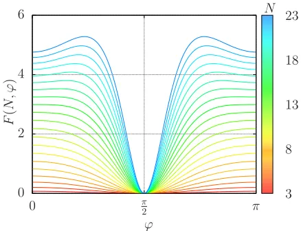
FIG. 2. Fisher information as a function of the parameterϕ. Each curve shows a different number of time stepsN, as illustrated by the key. Here the free parameters are chosen to beA=0.9 andb=0.1. We see a steady increase in the Fisher information for all values ofϕ. However, the peak value seems to move closer toπ /2 asNincreases.
same result will follow. In this case bothK2
0,1are proportional
to the identity K2
x =λ2x1, so that Pϕ(x)=tr(Kx2ρ)=λ2x for
any normalizedρ.
2. An example with enhanced precision
In the following, we consider a single qubit with parameter-dependent resetting. More concretely, we reset into a state that is a function of a parameterϕand whose measure-ments can be described by
K0 =
1 0
0 A ,
K1 =
0 cos(ϕ)√1−A2
0 sin(ϕ)√1−A2
, (26)
with 0A1. Furthermore, we may choose an initial state given by the density matrix
ρ =b|0 0| +(1−b)|1 1|, (27)
where 0b1. One can easily check that the above Kraus operators satisfy the completeness relation in Eq. (9) but do not commute:
[K0,K1]=0. (28)
Immediately, it should be noted that in general for this choice of Kraus operators, Eq. (12) is different to Eq. (13). Thus, these Kraus operators have potential to provide a Fisher in-formation with greater than linear scaling. In the next section, we will have a closer look at a possible implementation of the aboveK0andK1.
10−8
10−7
10−6
2 5 10 20
F
(
N
)
N F(N)
N2-scaling
[image:7.608.61.283.68.226.2]N-scaling
FIG. 3. Fitted log-log plot of the Fisher information for the Kraus operators given in Eq. (31) forϕ=(499/500)π and with A≈1, such that √1−A2=10−4. The trend is clearly not linear and is therefore beyond the standard linear scaling of classical systems. Plots showing scaling as∼N2and
∼Nare shown for illustration.
achieved when the parameter Ain Eq. (26) is close to unity, while the choice ofboffers little physical interest in long term scaling. In this case, we find thatF(N) scales as
F(N)∼(N2−N+c), (29)
where cis a small constant (cf. Figs.3and4). For largeN, the right-hand side of Eq. (29) is dominated by theN2 term
which implies scaling approaching the Heisenberg limit. The numerical simulations moreover show that
F(N, ϕ)=cos2(ϕ)(N2−N+c) (30)
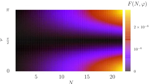
to a very good approximation. For example, Fig. 3 shows
F(N, ϕ) for a fixed value ofϕ. Figure4, which showsF(N, ϕ) forϕ∈(0, π), clearly demonstrates a nonlinear growth.
In general, for most values of A, the Fisher information grows nonlinearly withN initially but assumes linear scaling in N for large N. Only when the parameter A is close to one, the Fisher information is nonlinear for a relatively wide range of N. Our simulations show that enhanced scaling
F(N, ϕ)
5 10 15 20
N
0
π 2
π
ϕ
0
10−6
2×10⁻⁶
FIG. 4. Fitted function of the Fisher information for the scheme described by the Kraus operators in Eq. (31), again taking
√
1−A2=10−4. We see that the Fisher information is maximised around 0 andπand also appears to grow nonlinearly at these points, as shown in Fig.3.
which overcomes the standard quantum limit can be generated with no entanglement. The exact behavior that results from varying the parameterAis not studied here, though presents a potentially interesting topic on how this affects the long-term scaling as a function ofT. For instance, we know that taking values ofAincreasingly close to 1 results in more persistent Heisenberg-scaling, but its asymptotic limit is not determined. In all the finite cases considered here the scaling eventually reaches that of the standard quantum limit, but still offers an enhancement for someT. This result supports our earlier results in Ref. [29], where we analyze a much more complex system with applications in quantum metrology. There is no reason why a quantum system occupying a larger Hilbert space should not persist with enhanced scaling further even for very large values ofN. Unfortunately, numerical calcula-tions of the Fisher information are in general difficult to obtain in these complex systems. However, what we have seen here is that enhanced scaling is possible in such systems.
Moreover, we have seen in this section, that there are necessary (although not sufficient) conditions for producing a quantum enhancement. First, the Kraus operators should depend on ϕ in a nontrivial way. Second, Kraus operators which correspond to different measurement outcomes should not commute with each other which is a necessary criteria for strong temporal correlations in the measurement statistics. This observation can be used to guide the design of quan-tum jump metrology schemes which can then be analyzed for instance numerically via the simulation of the proposed measurement scheme.
IV. DETAILED ANALYSIS OF A CONCRETE PHYSICAL IMPLEMENTATION
To obtain more insight into how this works, we finally have a closer look at a possible concrete implementation of Eq. (26) and for which we can obtain analytical results. Suppose a single two-level atom is allowed to freely decay, while being subjected to parameter-dependent back-action upon photon emission. Such parameter-dependent queries could be realised physically by connecting the photodetectors that monitor the radiation field around the atom to a laser directed towards the atom. The laser sends a feedback pulse to the atom whenever a photon is detected. Most importantly, the laser parameters of the feedback pulse should depend on the unknown parameter
ϕthat we want to measure. In this case only the Kraus operator
K1would beϕ-dependent. There are a number of ways such
a scheme could be implemented but we focus on the resulting behavior here.
Proceeding as described, for example, in Refs. [37–39,52] and as we shall see below, we find that the dynamics of such a two-level atom with ground state|0and an excited state|1
over a short time intervalt can be described by the Kraus operators
K0 = |0 0| +e−12Ŵt|1 1|,
K1 =√Ŵt[cos(ϕ)|0 1| −isin(ϕ)|1 1|]. (31)
[image:7.608.55.295.552.689.2]subsection we see that the quantum trajectories of the atom are due to the successive application of the above Kraus operators on a coarse grained time scalet. To measure the unknown parameter ϕ, we observe the average number ¯N(T, ϕ) of photons emitted by the atom in a time interval (0,T) of length
T which we derive later in this section. Eventually, we show that this quantity may provide an enhanced measurement of the unknown parameterϕ.
Notice also that the Kraus operatorsK0andK1in Eq. (31) coincide with the Kraus operators in Eq. (26) forA=e−1
2Ŵt
in the limit of frequent measurements on the free radiation field which implies small time intervalst. The Kraus opera-torsK0andK1in Eq. (31) are in fact the Kraus operators used in Figs.3and4to allow for a comparison with the results in this section.
A. Quantum jump operators in open quantum systems
From quantum optics, we know that an atom that is con-stantly monitored but does not emit a photon evolves with the conditional Hamiltonian [37–39]
Hcond = −i
2h¯Ŵσ
+σ−, (32)
which is non-Hermitian. If no photon is detected for a short timet, the state of the atom evolves into the unnormalized state
|ψI(t+t) =exp (−iHcondt/h¯)|ψI(t) (33)
up to first order int. The normalization of this state squared equals the probability for no photon emission in (t,t+t). Hence, the no-photon time evolution of the atom automati-cally implements the transformation|ψI −→K0|ψIwithK0
given in Eq. (31), as long astis sufficiently small. This can be shown by calculating the right-hand side of Eq. (33).
Whenever a photon is detected, the atom is subsequently found in its ground state|0. Moreover, we know that the prob-ability density for the emission of a photon is the product of its spontaneous decay rateŴand the population1|ψ(t)2 in the excited state. Suppose now, every photon emission triggers a short strong laser pulse which transfers its state into a state of the form
|ψph =cos(ϕ)|0 −isin(ϕ)|1, (34)
which could be achieved in a variety of ways. Then the change of atomic state in the case of an emission can be described by the Kraus operatorK1in Eq. (31).
B. Average number of emitted photons
To determine the unknown parameterϕ, we utilize in the following a measurement of the average number of emitted photons in a time period (0,T), denoted ¯N(T, ϕ). In this subsection, we calculate this observable for the proposed experimental setup. To do so, we notice that ¯N(T, ϕ) can be written as
¯
N(T, ϕ)=
∞
n=1
npn(0,T), (35)
where pn(0,T) is the probability of the system emitting
exactlynphotons in a time interval (0,T) for a given initial state. For simplicity, we assume in the following that the state of the atom at the timet =0 equals the the reset state after a photon detection|ψph
which can be found in Eq. (34). Next we notice that the time evolution operator of our two-level system under the condition of no photon detections equalsUcond(T,0)=exp(−iHcondT/h¯) and that the probabil-ity of the system not emitting a photon in a time period (0,T),
p0(0,T) is given by
p0(0,T)= Ucond(T,0) |ψph 2
=cos2(ϕ)+e−ŴTsin2(ϕ). (36)
Moreover, one can show that the probability density for emit-ting exactly one photon in a time period (0,T) at a timet
equals the probability densityw1(0,t) for the emission of a first photon at a timet,
w1(0,t)= −
d
dtp0(0,t)=Ŵsin 2
(ϕ)e−Ŵt, (37)
multiplied by the probability for no photon emission in (t,T), which we denote p0(t,T). The probability p1(0,T) of the system emitting exactly one photon in a time period (0,T) is hence obtained by integrating these probability densities over
t. Hence,
p1(0,T)= T
0
dtw1(0,t)p0(t,T). (38)
Proceeding analogously and calculating the probability for exactlynphoton emissions in a time interval (0,T) moreover yields
pn(0,T)=
T
0
dt1w1(0,t1)pn−1(t1,T), (39)
where pn−1(t1,T) denotes the probability for the emission
of n−1 photon in the time interval (t1,T). In other words,
the probability for having n photons in (0,T) is the sum of all probability densities with a first photon att1 ∈(0,T) and exactlyn−1 photons in (t1,T). In the following, we use this relation to determinepnas a function ofw1andp0.
Iteration of Eq. (39) yields
pn(0,T)=
T
0 dt1
T
t1
dt2w1(0,t1)w1(t1,t2)pn−2(t2,T)
(40)
and so on. Hence,
pn(0,T)=
T
0 dt1
T
t1 dt2· · ·
T
tn−1
dtnw1(0,t1)
×w1(t1,t2). . .w1(tn−1,tn)p0(tn,T)
= n
i=1
T
ti−1
dtiw1(ti−1,ti) p0(tn,T), (41)
meaning
lim
T→∞
T
ti−1
dtiw(ti−1,ti)=sin2(ϕ),
lim
T→∞p0(tn,T)=cos
2
(ϕ). (42)
Hence, we find that the probability for n photons in the stationary limit is given by
lim
T→∞pn(0,T)=sin
2n
(ϕ) cos2(ϕ). (43)
The average number of photons emitted in the stationary limit can now be calculated by substituting Eq. (43) into Eq. (35), which gives
¯
N(∞, ϕ)=
∞
n=1
nsin2n(ϕ) cos2(ϕ). (44)
This is nearly a geometric series. After appropriately modify-ing the standard geometric series, it can be shown that
∞
n=1
nrn = r
(1−r)2. (45)
Takingr=sin2(ϕ), we hence find
¯
N(∞, ϕ)=tan2(ϕ). (46)
This function matches expectations, as we see that for the case where the system is reset exactly to the excited state, we see an infinite number of photons, whereas when it is reset to the ground state we see no photons.
For the purposes of metrology, we want a signal we can scale with time. As such, we can calculate how this signal scales for finiteT. By not imposingT → ∞, the integrals no longer factorize nicely. Nevertheless, a solution can still be found forp(n,T), which is given by
pn(0,T)=sin2n(ϕ) cos2(ϕ)+
e−ŴTsin2n
(ϕ)
n!
×
(ŴT)n−cos2(ϕ)
n
m=0 n!
m!(ŴT)
m
. (47)
The derivation of Eq. (47) is given in the Appendix. The limit of the sum in Eq. (35) wheren→ ∞is now more difficult to resolve. Although the limit is well defined, it is not straightfor-ward to explicitly calculate. Hence, for simplicity, all results involving this term will be approximated by choosing a large finite value forn. In doing so, ¯N(T, ϕ) can be calculated to a very good approximation. In Fig.5, we see how this function behaves as a function ofϕat a variety of timesT.
This signal clearly displays dependence on the parameter
ϕ that grows in time. Hence, it should be possible to use this signal to extract information about ϕ. To calculate the uncertainty inϕ, we use the error propagation formula [22]
(ϕ)2 = [A(ϕ)] 2
dAdϕ
2 , (48)
for some signal A(ϕ) that has dependence on the unknown parameter ϕ. For our case of A=N¯, the variance in the
0 2 4 6 8 10
0 π
2 π
¯N
ϕ
T=2Γ−1
T=4Γ−1
T=6Γ−1
T=8Γ−1
T=10Γ−1
[image:9.608.327.545.72.223.2]T→∞
FIG. 5. The plot of ¯N now does not go to infinity, as a finite amount of time is considered. The curve has a similar functional shape to the case of infinite time and hence demonstrates the validity of the calculations. Here, the sum is taken up ton=2000. The limit ofT → ∞calculated in Eq. (46) is also shown for consistency.
numerator is given by
(N¯)2 =
∞
n=1
n2pn(0,T)−
∞
n=1
npn(0,T)
2
, (49)
from Eq. (35), while the derivative in the denominator can be calculated straightforwardly.
Plotting as a function of ϕ for a variety of times T, we see in Fig. 6 how the uncertainty in ϕ changes in time. In particular, the error decreases in time. However, it appears to approach a fixed point that depends on the value ofϕ being considered. Also, the error is able to reach a lower value for a large amount of time the closer it is toπ /2. Hence, to maximise the scaling it appears that we should choose a value ofϕclose toπ /2, so long as a large timeTmay be considered. As such, whenT is unable to be taken as a large value, a value ofϕ away fromπ /2 is preferable. Takingϕ as values close toπ /2, we now plot (ϕ)2 as a function of timeT. This is
0 0.5 1 1.5 2
0 π
2 π
(∆
ϕ
)
2
ϕ T=Γ−1
T=2Γ−1
T=5Γ−1
T=8Γ−1
[image:9.608.328.544.536.692.2]T=15Γ−1
10−6
10−4
10−2
1 102
104
0.1 1 10 100
(∆
ϕ
)
2
T (units of Γ−1
) H-berg scaling
SQL scaling
ϕ= 1.5
[image:10.608.62.282.71.228.2]ϕ= 1.4
FIG. 7. The uncertainty (ϕ)2 as a function ofT plotted for fixed values ofϕ (ϕ=1.4,1.5). For illustrative purposes, scaling according to the standard quantum limit (∼1/T) and the Heisenberg limit (∼1/T2) are shown. We see that the scaling of our system lies between these two. The results are produced with a sum up to
n=2000 again.
shown in Fig.7. Here, we see the scaling is surpassing that of the standard quantum limit.
Crucially, we see that there is an enhanced scaling present for this measurement scheme. Although this measurement is not necessarily an optimum measurement, it serves as a proof-of-principle that an enhanced time-dependent scaling can be found for a relatively simple system with quantum feedback. Indeed, there are many ways in which this system can be developed further, including going to a larger system size or performing a more complex measurement, such as using photon correlations where an enhancement has already been shown [29]. In Fig.7, we see that the uncertainty inϕ seems to be levelling off to a fixed value. This is also suggested in Fig.6for other values ofϕ. If we move to a larger system size, then the overall uncertainty should be reduced further. This is because in a larger system size two initially close together
10−2
10−1
1 101
1 10 100
(∆
ϕ
)
2
T (units of Γ−1
)
ϕ= 1.25
ϕ= 1.3
ϕ= 1.35
ϕ= 1.4
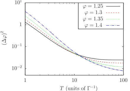
FIG. 8. Uncertainty (ϕ)2as a function ofT plotted for a range of values ofϕ. For smaller values ofϕ, we see the long time limit of plateauing behavior both more clearly and earlier. This shows how values ofϕthat are initially optimal in the short time limit eventually become inferior to others in the long time limit. The results are produced with the same simulations as previous plots in this section.
points in the relevant space can move further away from each other and hence become more distinguishable.
Another observation from Figs. 6 and7 is that for small
T a value of ϕ closer to 0 is preferable. However, as T
increases, the optimum value of ϕ to be measured shifts asymptotically closer to π /2. This supports what was seen earlier in Fig.2, where the maximum of the Fisher information moves closer to π /2 with increasingN. Indeed all values of
ϕtend to follow a standard quantum limit scaling initially for this measurement scheme, before eventually at some timeT
gaining some enhanced scaling and ultimately then plateauing at some fixed value for (ϕ)2. This allows one to determine
an optimum value of ϕ to measure ifT becomes a limiting factor. This is shown for a range of values ofϕin Fig.8.
V. CONCLUSIONS
This paper introduces the general concept of quantum jump metrology, which is based on generalized sequential measurements and considers the total durationT of the mea-surement process as the main meamea-surement resource. One way of implementing quantum jump metrology is to apply quantum feedback to open quantum systems. It is shown that this approach can indeed result in precision scaling beyond the standard quantum limit without the need for complex state preparation. This is in contrast to closed quantum systems, where overcoming the standard quantum limit requires en-tanglement or the presence of other highly nonclassical states which are hard to prepare experimentally. Open quantum sys-tems therefore currently receive a lot of attention in quantum metrology but their systematic study is often difficult, since standard quantum metrology techniques do not extend easily to more complex systems [32].
Here we provide novel insight into quantum metrology with generalized sequential measurements by drawing analo-gies to hidden quantum Markov models [47–51]. This anal-ogy suggests that there could be a wide range of computa-tional advantages compared to analogous classical machines [48,53,54,56]. As usual, we describe the system dynamics induced by the generalized measurements with Kraus oper-ators. For applications in quantum metrology, these should depend in a nontrivial fashion on the parameter ϕ that we want to measure. Moreover, the Kraus operators associated with different measurement outcomes should not commute with each other. A quantum enhancement of the scaling of errors can be expected, when measurement sequences cannot be modeled as Markov processes and contain long-range tem-poral correlations. The above described necessary (although not sufficient) conditions can be used to guide the design of quantum metrology schemes in open quantum systems.
[image:10.608.64.284.525.680.2]numerical analysis of a more complex quantum metrology scheme based on the conditional dynamics of the coherent states of an optical cavity for which we were unable to establish analytical bounds for the precision of measurement outcomes [29].
We also emphasize again here that the approach and im-plementation shown are not necessarily optimum but provide a simple pathway to enhancements. There are other meth-ods that obtain enhancements that could potentially also be incorporated into this work, such as a final measurement of the system to obtain a further enhancement [58]. The scope for further developments of these schemes is large and should be of significant interest. Furthermore, as discussed in Sec. III C 2, there is still much more to explore in terms of the Fisher information of systems of this type, such as a more rigorous study involving varying the parameter A. We leave this as an open question here that remains to be investigated in future work. Overall, we hope that the general discussion of this paper helps the design of novel practical quantum metrology schemes.
ACKNOWLEDGMENTS
We acknowledge financial support from the Oxford Quan-tum Technology Hub NQIT (Grant No. EP/M013243/1). Statement of compliance with EPSRC policy framework on research data: This publication is theoretical work that does not require supporting research data.
APPENDIX: DERIVATION OFpn(0,T)
We derive Eq. (47) by direct construction. We start with the expression
pn+1(0,T)=
T
0
dtw1(0,t)pn(t,T). (A1)
Using the notation pn(0,t)=:pn(t) and w1(0,t)=:w1(t) and noting that pn(t,T)=pn(0,T −t)=:pn(T −t) the
convolution theorem yields
˜
pn+1(s)=w˜1(s) ˜pn(s)=w˜1(s)n+1˜p0(s), (A2)
where ˜g:=L[g] denotes the Laplace transform ofg. Applying the convolution theorem again then yields
pn+1(T)=(fn+1∗p0)(T), fn(t)=L−1[ ˜w1(s)n](t),
(A3)
where∗denotes the convolution product,
(f ∗g)(T) := T
0
dt f(t)g(T −t). (A4)
Using Eq. (37) we have
˜
w1(s)n+1=
Ŵn+1sin2(n+1)
(ϕ) (Ŵ+s)n+1
= Ŵ n+1
sin2(n+1)(ϕ) (−1)nn!
dn dsn
1
s+Ŵ
=L
Ŵn+1sin2(n+1)(ϕ)t
ne−Ŵt
n!
(s), (A5)
from which it follows that
fn+1(t)=Ŵn+1sin2(n+1)(ϕ) tne−Ŵt
n! . (A6)
Using this expression and Eq. (A3) we obtain
pn+1(T)=
Ŵn+1sin2(n+1)
(ϕ)
n!
e−ŴTTn+1sin2
(ϕ)
n+1
+cos2(ϕ)
T
0
dt tne−Ŵt
. (A7)
The integral in the above can be evaluated as
T
0
dt tne−Ŵt = 1
Ŵn+1[n!−γ(n+1, ŴT)], (A8)
where γ denotes a special function called the incomplete
γ-function, which is defined by
γ(a,y)= ∞
y
dz za−1e−z. (A9)
Using Eq. (A8) we obtain
pn+1(t)=sin2(n+1)(ϕ) cos(ϕ)
+(ŴT) n+1e−ŴT
sin2(ϕ) sin2(n+1)(ϕ) (n+1)!
−cos
2(ϕ) sin2(n+1)
(ϕ)
n! γ(n+1, ŴT)
=sin2(n+1)(ϕ) cos(ϕ)+(ŴT)
n+1e−ŴTsin2(n+1)
(ϕ) (n+1)!
−cos2(ϕ) sin2(n+1)(ϕ)
×
(ŴT)n+1e−ŴT
(n+1)! +
γ(n+1, ŴT)
n!
. (A10)
Using the definition Eq. (A9) and integration by parts one can prove inductively that
γ(n+1, ŴT)=e−ŴT n
m=0 n!
m!(ŴT)
m
. (A11)
We therefore obtain
pn+1(t)=sin2(n+1)(ϕ) cos(ϕ)
+(ŴT)
n+1e−ŴTsin2(n+1)
(ϕ) (n+1)!
−cos2(ϕ) sin2(n+1)(ϕ)
n+1
m=0
1
m!(ŴT)
m,
(A12)
[1] F. Wolfgramm, C. Vitelli, F. A. Beduini, N. Godbout, and M. W. Mitchell, Entanglement-enhanced probing of a delicate material system,Nat. Photonics7,28(2013).
[2] M. A. Taylor, J. Janousek, V. Daria, J. Knittel, B. Hage, H.-A. Bachor, and W. P. Bowen, Biological measurement beyond the quantum limit,Nat. Photonics7,229(2013).
[3] A. Crespi, M. Lobino, J. C. F. Matthews, A. Politi, C. R. Neal, R. Ramponi, R. Osellame, and J. L. O’Brien, Measuring protein concentration with entangled photons, Appl. Phys. Lett.100,
233704(2012).
[4] B. P. Abbottet al.(LIGO Scientific Collaboration and Virgo Collaboration), Observation of Gravitational Waves from a Bi-nary Black Hole Merger,Phys. Rev. Lett.116,061102(2016). [5] C. M. Caves, Quantum-mechanical noise in an interferometer,
Phys. Rev. D23,1693(1981).
[6] R. S. Bondurant and J. H. Shapiro, Squeezed states in phase-sensing interferometers,Phys. Rev. D30,2548(1984). [7] D. W. Berry and H. M. Wiseman, Optimal States and Almost
Optimal Adaptive Measurements for Quantum Interferometry,
Phys. Rev. Lett.85,5098(2000).
[8] C. C. Gerry, A. Benmoussa, and R. A. Campos, Nonlinear interferometer as a resource for maximally entangled photonic states: Application to interferometry,Phys. Rev. A66,013804
(2002).
[9] R. A. Campos, C. C. Gerry, and A. Benmoussa, Optical interfer-ometry at the Heisenberg limit with twin Fock states and parity measurements,Phys. Rev. A68,023810(2003).
[10] V. Giovannetti, S. Lloyd, and L. Maccone, Quantum-enhanced measurements: Beating the standard quantum limit, Science 306,1330(2004).
[11] V. Giovannetti, S. Lloyd, and L. Maccone, Quantum Metrology,
Phys. Rev. Lett.96,010401(2006).
[12] B. L. Higgins, D. W. Berry, S. D. Bartlett, H. M. Wiseman, and G. J. Pryde, Entanglement-free Heisenberg-limited phase estimation,Nature450,393(2007).
[13] S. D. Huver, C. F. Wildfeuer, and J. P. Dowling, Entangled fock states for robust quantum optical metrology, imaging, and sensing,Phys. Rev. A78,063828(2008).
[14] C. C. Gerry and J. Mimih, The parity operator in quantum optical metrology,Contemp. Phys.51,497(2010).
[15] C. C. Gerry, J. Mimih, and R. Birrittella, State-projective scheme for generating pair coherent states in traveling-wave optical fields,Phys. Rev. A84,023810(2011).
[16] J. Joo, W. J. Munro, and T. P. Spiller, Quantum Metrology with Entangled Coherent States,Phys. Rev. Lett.107,083601
(2011).
[17] M. Zwierz, C. A. Perez-Delgado, and P. Kok, Ultimate limits to quantum metrology and the meaning of the Heisenberg limit,
Phys. Rev. A85,042112(2012).
[18] K. Jiang, C. J. Brignac, Y. Weng, M. B. Kim, H. Lee, and J. P. Dowling, Strategies for choosing path-entangled number states for optimal robust quantum-optical metrology in the presence of loss,Phys. Rev. A86,013826(2012).
[19] P. A. Knott, W. J. Munro, and J. A. Dunningham, Attaining sub-classical metrology in lossy systems with entangled coherent states,Phys. Rev. A89,053812(2014).
[20] R. Carranza and C. C. Gerry, Photon-subtracted two-mode squeezed vacuum states and applications to quantum optical interferometry,JOSA B29,2581(2012).
[21] A. De Pasquale, P. Facchi, G. Florio, V. Giovannetti, K. Matsuoka, and K. Yuasa, Two-mode Bosonic quantum metrology with number fluctuations,Phys. Rev. A92,042115
(2015).
[22] J. P. Dowling and K. P. Seshadreesan, Quantum optical tech-nologies for metrology, sensing, and imaging, J. Lightwave Technol.33,2359(2015).
[23] P. Kok and B. Lovett,Introduction to Optical Information Quan-tum Processing QuanQuan-tum information processing(Cambridge University Press, Cambridge, 2010).
[24] S. L. Braunstein and C. M. Caves, Statistical Distance and the Geometry of Quantum States,Phys. Rev. Lett. 72, 3439
(1994).
[25] S. Boixo, A. Datta, S. T. Flammia, A. Shaji, E. Bagan, and C. M. Caves, Quantum-limited metrology with product states,Phys. Rev. A77,012317(2008).
[26] D. Braun and J. Martin, Heisenberg-limited sensitivity with decoherence-enhanced measurements, Nat. Commun. 2, 223
(2011).
[27] M. Guta, Fisher information and asymptotic normality in sys-tem identification for quantum Markov chains,Phys. Rev. A83,
062324(2011).
[28] D. Burgarth, V. Giovannetti, A. N. Kato, and K. Yuasa, Quan-tum estimation via sequential measurements,New J. Phys.17,
113055(2015).
[29] L. A. Clark, A. Stokes, and A. Beige, Quantum-enhanced metrology through the single mode coherent states of optical cavities with quantum feedback, Phys. Rev. A 94, 023840
(2016).
[30] K. Macieszczak, M. Guta, I. Lesanovsky, and J. P. Garrahan, Dynamical phase transitions as a resource for quantum en-hanced metrology,Phys. Rev. A93,022103(2016).
[31] A. H. Kiilerich and K. Mølmer, Bayesian parameter estimation by continuous homodyne detection,Phys. Rev. A94, 032103
(2016).
[32] D. Braun, G. Adesso, F. Benatti, R. Floreanini, U. Marzolino, M. W. Mitchell, and S. Pirandola, Quantum enhanced mea-surements without entanglement,Rev. Mod. Phys.90,035006
(2018).
[33] S. Oppel, T. Büttner, P. Kok, and J. von Zanthier, Super-Resolving Multi-Photon Interferences with Independent Light Sources,Phys. Rev. Lett.109,233603(2012).
[34] M. E. Pearce, T. Mehringer, J. von Zanthier, and P. Kok, Precision estimation of source dimensions from higher-order intensity correlations,Phys. Rev. A92,043831(2015). [35] L. A. Clark, F. Torzewska, B. Maybee, and A. Beige,
Non-ergodicity in open quantum systems through quantum feedback,
arXiv:1611.03716.
[36] F. Albarelli, M. A. C. Rossi, D. Tamascelli, and M. G. Genoni, Restoring Heisenberg scaling in noisy quantum metrology by monitoring the environment,Quantum2,110(2018).
[37] G. C. Hegerfeldt, How to reset an atom after a photon detection: Applications to photon-counting processes,Phys. Rev. A47,
449(1993).
[38] J. Dalibard, Y. Castin, and K. Mølmer, Wave-Function Ap-proach to Dissipative Processes in Quantum Optics,Phys. Rev. Lett.68,580(1992).
[40] H.-P. Breuer and F. Petruccione,The Theory of Open Quantum Systems(Oxford University Press, Oxford, 2002).
[41] H. M. Wiseman and G. J. Milburn,Quantum Measurement and Control(Cambridge University Press, Cambridge, 2010). [42] T. Baumgratz, M. Cramer, and M. B. Plenio, Quantifying
Coherence,Phys. Rev. Lett.113,140401(2014).
[43] K. Kraus, States, Effects, and Operations, Lecture Notes in Physics, Vol. 190 (Springer-Verlag, Berlin, 1983).
[44] L. R. Rabiner, A tutorial on hidden Markov models and selected applications in speech recognition,Proc. IEEE77,257(1989). [45] H. Xue, Hidden Markov models combining discrete symbols
and continuous attributes in handwriting recognition, IEEE Trans. Pattern Anal. Mach. Intell.28,458(2006).
[46] B. Vanluyten, J. C. Willems, and B. D. Moor, Equivalence of state representations for hidden Markov models,Syst. Control Lett.57,410(2008).
[47] K. Wiesner and C. P. Crutchfield, Computation in finitary stochastic and quantum processes,Physica D237,1173(2008). [48] A. Monras, A. Beige, and K. Wiesner, Hidden quantum Markov models and non-adaptive read-out of many-body states,Appl. Math. and Comp. Sciences3, 93 (2011).
[49] M. Schuld, I. Sinayskiy, and F. Petruccione, An introduction to quantum machine learning,Contemp. Phys.56,172(2014). [50] J. Biamonte, P. Wittek, N. Pancotti, P. Rebentrost, N. Wiebe,
and S. Lloyd, Quantum machine learning, Nature 549, 195
(2017).
[51] J. Barry, D. T. Barry, and S. Aaronson, Quantum partially ob-servable Markov decision processes,Phys. Rev. A90,032311
(2014).
[52] L. A. Clark, W. Huang, T. M. Barlow, and A. Beige, Hidden quantum Markov models and open quantum systems with in-stantaneous feedback, inProceedings of the Interdisciplinary Symposium on Complex Systems, Emergence, Complexity and Computation (ISCS’14)(Springer, Berlin, 2015), p. 143. [53] H.-C. Cheng, M.-H. Hsieh, and P.-C. Yeh, The learnability of
unknown quantum measurements, QIC16, 0615 (2016). [54] S. Srinivasan, G. Gordon, and B. Boots, Learning hidden
quantum Markov models, inProceedings of the Twenty-First International Conference on Artificial Intelligence and Statis-tics(PMLR, Playa Blanca, Lanzarote, Canary Islands, 2018), Vol. 84, pp. 1979–1987.
[55] P. Rebentrost, T. R. Bromley, C. Weedbrook, and S. Lloyd, Quantum Hopfield neural network,Phys. Rev. A98,042308
(2018).
[56] C. Aghamohammadi, J. R. Mahoney, and J. P. Crutchfield, Extreme quantum advantage when simulating classical systems with long-range interactions,Sci. Rep.7,6735(2017). [57] R. Blatt and P. Zoller, Quantum jumps in atomic systems,Eur.
J. Phys.9,250(1988).
[58] A. H. Kiilerich and K. Mølmer, Hypothesis testing with a continuously monitored quantum system, Phys. Rev. A 98,