System identification and control of a 3D truss structure using PLID and LQG

Rochester Institute of Technology

RIT Scholar Works

Theses

Thesis/Dissertation Collections

10-1-1997

System identification and control of a 3D truss

structure using PLID and LQG

Phillip Vallone

Follow this and additional works at:

http://scholarworks.rit.edu/theses

This Thesis is brought to you for free and open access by the Thesis/Dissertation Collections at RIT Scholar Works. It has been accepted for inclusion in Theses by an authorized administrator of RIT Scholar Works. For more information, please [email protected].

Recommended Citation

ROCHESTER INSTITUTE OF TECHNOLOGY

Rochester, New York

October, 1997

SYSTEM IDENTIFICATION AND CONTROL OF A 3D TRUSS STRUCTURE

USING PLID AND LQG

A THESIS FOR M.S.

SUBMITTED TO

THE FACULTY OF THE DEPARTMENT OF ELECTRICAL ENGINEERING

IN CANDIDACY FOR THE DEGREE OF

MASTER OF SCIENCE

in

ELECTRICAL ENGINEERING

BY

PHILLIP VALLONE

Approved

By:

Prof.

Dr. Mark A. Hopkins

(Thesis Advisor)

Prof.

Dr. Mark H.

Kempski

Prof.

Dr. Athimoottil V. Mathew

Prof.

RIT Thesis Binding Procedure

Examples of Thesis Reproduction Permission Statement

(3 options--please choose one)

Permission granted

T~.tleofthesis

S,j.:>t'XM

J:AQvJ\',r'<"'~~'Qh

o,vv\

(0;1[0\

of

~

51)

lrv.s~

>-t-,..v,--\vr~

VSI1I\'tl

ELlc>

"""&

LOh

I, author's name,

hereby grant permission to the Wallace Library of the Rochester Institute of Technology

to reproduce my thesis in whole or in part. Any reproduction will not be for commercial use or profit.

Date: \

1.)

_r.l

g

/q

_'--'--

7

Signature of Author:

-OR

Permission From Author Required

Title of thesis

_

I, author's name,

prefer to be contacted each time a request for reproduction is made.

If

permission is granted,

any reproduction will not be for commercial use or profit. I can be reached at the following address:

Phone:

_

Date:

Signature of Author:

_

OR

Permission Denied

Title of thesis

_

I, author's name,

hereby deny permission to the Wallace Library of the Rochester Institute of Technology

to reproduce my thesis in whole or in part.

ACKNOWLEDGMENTS

I am _sincerely grateful to Dr. Mark Hopkins for his patience

and guidance in

teaching

me the ins and outs of his algo

rithm. His open exchange of expertise was a _refreshing and

rewarding experience I shall never forget.

Finally,

to _my wife

Nancy

and son Maxwell goes a great sense of debt and appreciation for their patience and

loving

sup

port. The hot chocolate sustained me through those

long

nights of "basement exile". Without their encouragement, I

TABLE OF CONTENTS

Page

Abstract vi

List of Tables viii

List of Figures ix

Introduction 1

1. 0 Review of Literature 8

1. 1 A Fast Method 8

1. 2 A Method for Large Systems 19

2. 0 Testbed Description 23

2. 1 Design Criterion 23

2. 2 Testbed Design 24

2.2.1

Geometry

24

3. 0 Digital Controller 29

3. 1 System Description 29

3. 2 Power Amps 32

3. 3 Noise Sources 37

3.3.1 A/D and D/A Converters 37

3.3.2 Sensors 38

4.0 System Identification Algorithm Description 40

4. 1 Overview of PLID 40

4. 2 Mathematical Framework 45

4.2.1 Extended State Model Definition 45

4.2.2 Stochastic Extended State Model 50

4.2.3 PLID Equations 55

5. 0 MATLAB Simulation Results 65

5. 1 Direct Implementation of PLID 65

5.1.1 Test Model 1 65

5.1.2 Test Model 2 71

5.2 Square Root Filter Implementation of PLID 73

5.2.1 Full Order Test Model 3 74

5.2.2 Reduced Order Models: 9 Modes 81

5.2.3 Reduced Order Models : 12 Modes 84

6. 0 PLID Testbed Results 98

6.1 MIMO Models 102

6.1.1 Initial Results 102

6.1.2 Refined Results 108

6.2 SIMO Models 112

6.2.1 Initial Results 112

6.2.2 Refined Results 118

7. 0 Conclusions 144

8 . 0

Summary

149

References

Appendix

A) MATLAB Code

Al)

Directly

Coded PLID Al-1 to Al-41

A2) PLID Square Root Filter Code . . . . A2-1 to A2-69

B) C Code for Data Acquisition Bl to B21

C) Drawings of Testbed Cl to CIO

D) NASTRAN Model Data Deck Dl to D13

E) Power

Amp

Schematic El

G) IFORSELS

Theory

G1-G7

H) Testbed Design H1-H26

H2. 1) Testbed Design Criterion HI

-H3

H2. 2

)

Testbed Design H4

-H5

H2 .

3)

Instrumentation H6

-HI 8

H2.3.1) Sensors H6

-H10

H2.3.2) Actuators Hll

-H18

H2.3.2.1) PZT Equations Hll

-H18

H2.4) NASTRAN Analysis H19

-H26

H2.4.1) Brief Intro, to NASTRAN .... HI 9

-H21

H2.4.2) Model Description H21

-H23

H2.4.3) Sensor & Actuator

Modeling

. H24

ABSTRACT

Thisthesis dealswiththe experimental application of a systemidentificationtech

nique called pseudo-linear identification (PLID). PLID is a

discrete-time,

_multi-input,

multi-output

(MEMO),

state _space, simultaneous parameter estimator and one _step ahead

state predictor oflinear time invariant systems. No measurements are assumed perfect

under

PLED;

thatistheinputs and outputs are allowedto havezero mean white gaussian

(ZMWG)

additive noise.

Furthermore,

the states are also assumed to have additive

ZMWGnoise.

Like most systemidentification

techniques,

PLED requires the systemto be com

pletely controllable and observable under the given actuator and sensor suite. _{The only}

firm assumption made on model structureis that the transferfunction be _{strictly proper;}

that

is,

the

frequency

response is

bounded

and tends towards zero as

frequency

is in

creasedtoinfinity. Poleand zero locationsare not _confined;

indeed,

unstable systems can

be

identified,

and

furthermore,

they

canbe controlled becausePLED provides simultane

ous one _step ahead state predictions. Developed

by

Hopkins et. al. in 1988

[1],

this

method has seenlittle application(due in part to its youth);

however,

it is shown in the

following

pages tobe a powerful technique_{for performing} state space system identifica

tion,

aswellas on-line model order reduction.

The experiment involves _{applying PLED} toa 3-Dimensional

(3-D)

kinematic truss

structure (referred to here forward as the

"testbed")

in a

batch

mode (off-line). Batch

mode

identification,

by

definition,

implies that the testbed does not change _appreciably

betweenthe time itwas identified andthe time itwill be controlled. Formost

kinematic

structures, this is true. PLED can be used for real-time

(on-line)

system

identification.

and the

high

bandwidth of control (hundreds of

hertz),

this is not possible with current

personalcomputer

(PC)

based

controllers.

Ultimately,

the state space model generated

by

PLED will be used to design a closed

loop

controller forthe testbed thatwill increase its

damping

twenty

fold,

from _ap

proximately 0.25% zetato 5% zeta. Dueto time constraints, we will _only show simula

tionresults oftheclosed

loop

system.

List of Tables

Page

Table

3.2-1)

Pole/ZeroLocations ofPA-85 Witha luF Load 34

List of Figures

Page

1-1)

Bode

Results,

Red-o=

EDd,

Green=_Actual

Plant,

s/n= _{lOOdB 9}

1_-2)

PZ-Map Results,

Red=

EDd,

Green=_Actual

Plant,

s/n= _{1 OOdB 10}

1-3)

Bode

Results,

Red-o=

EDd,

Green=_Actual

Plant,

s/n=_{60dB 1 1}

1-4) PZ-Map Results,

Red=

EDd,

Green=_Actual

Plant,

s/n=_{60dB 1 1}

1-5)

Bode

Results,

Red-o

=

EDd,

Green=_Actual

Plant,

s/n=_{50dB 12}

1_-6)

PZ-Map

Results,

Red=

EDd,

Green=_Actual

Plant,

s/n= _{50dB 13}

1-7)

Bode

Results,

Red-o=

EDd,

Green=

Actual

Plant,

s/n=_{30dB 14}

1-8) PZ-Map

Results,

Red=

EDd,

Green=_Actual

Plant,

s/n= _{30dB 14}

1-9)

Bode

Results,

Red-o=

EDd,

Green=_Actual

Plant,

s/n=_{50dB 15}

1-10)

Bode

Results,

Red-o=

EDd,

Green=

Actual

Plant,

s/n=

90dB,

36states... 16 1-1

1)

PZ-Map

Results,

Red=

EDd,

Green=_Actual

Plant,

s/n=

90dB,

36states... 17

1-12)

Bode

Results,

Red-o=

EDd,

Green=

Actual

Plant,

s/n=

60dB,

36states... 18

1-13) PZ-Map

Results,

Red=

EDd,

Green=_Actual

Plant,

s/n

-60dB,

36 states... 18

2-1)

EFORSELS Algorithm Basic Flow Diagram 20

Fig.

2.2-1)

Rough SketchofStructure 24

Fig.

2.2.1-1)

Top

View Line DrawofStrutsandUpper Delta Frame 25

Fig.

2.2.1-2)

SideViewofTestbed 26

Fig.

2.2.1-3)

Cut-away

ofSquare Actuator Adapter SectionofSupportTubes 27

Fig.

3.1-1)

PartialTimeline onPC using MS-DOS 31

Fig. 3.2-1)Open

Loop

Gain PlotofthePA-85 Witha luTLoad 35

Fig.

3.2-2)

Open

Loop

Gain Plot With Compensation

RcCc

36

Fig.

3.2-3)

Open

Loop

Gain Plot With Compensation&FeedbackPole 36

Fig. 5.1.1

-1

)

Maximum AbsoluteParameterand State Prediction Error- Noiseless 67

Fig.

5.1.1-2)

State|Actual-_One

Step

_{AheadPrediction|: Noiseless 68}

Fig.

5.1.1-3)

Actual

(red)

vs.Estimated

(green)

Transfer Functions- Noiseless 68

Fig.

5.1.1-4)

Actual

(red)

vs. Estimated

(green)

Transfer Functions- _s/n=28dB 70

Fig. 5.

1.2-1)

ConvergencePlotforModel 2with6dB s/n 71

Fig.

5.2.1-1)

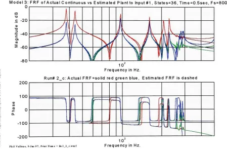
MagnitudeandPhaseBodePlotforModel

3,

ContinuousTime 75

Fig.

5.2.1-2)

BodePlotforModel 3 ActualContinuousPlantvs. Estimated Discrete ....76

Plant

Fig.

5.2.1-3)

Bode Plot for Model 3 Actual Discretized

(ZOH)

vs.Estimated Discrete...77

Plant

Fig.

5.2.1-4)

Bode PlotforModel 3 ActualDiscretized

(ZOH)

vs.Estimated Discrete... 78

Plant

Fig.

5.2.1-5)

Max. Sensor Prediction ErrorforModel 3 79

Fig.

5.2.2-1)

MagnitudeandPhase Bode PlotforModel

3,

18 StateEDdModel 81

Fig.

5.2.2-2)

Max. Sensor Prediction Error for Model

3,

18 States 82

Fig.

5.2.2-3)

MagnitudeandPhase Bode Plot for Model

3,

18 State EDd

Model,

Low...83

Noise

Fig.

5.2.3-1)

Max. Sensor Prediction Error for Model

3,

24states 84

Fig.

5.2.3-2)

MagnitudeandPhase Bode PlotforModel

3,

24StateEDd

Model,

85

LowNoise

Fig.

5.2.3-3)

One-step-aheadSensor Predictionvs. ActualOutputModel

3,

24 States...86

Fig.

5.2.3-4)

Magnitude&Phase BodePlot for Model

3,

24 StateEDd

Model,

87

Low Noise 3200samples

Fig.

5.2.3-5)

PZ

Map

ofModel

3,

24 State ED Model BeforeandAfter Stabilization 89

Fig.

5.2.3-6)

Magnitude&PhaseBodePlotforModel

3,

Unstablevs. Stabilized 90

Estimate

Fig.

5.2.3-7)

ActualSensor

(green--)

vs.Kalman

Est.,

Model

3,

23 StateModel 91

Fig.

5.2.3-8)

ActualSensor

(green-)

vs. Kalman

Est.,

Model

3,

23 State Model 92

Fig.

5.2.3-9)

Magnitude& PhaseBodePlot forModel

3,

Openvs. Closed

Loop

93

Fig.

5.2.3-10)

Magnitude & Phase Bode PlotforModel

3,

Openvs. Closed 94

Fig. 5.2.3-1

1)

Open

Loop

Sensor Output

(green--)

vs. Closed

Loop,

Model

3,

95 23 StateModel

Fig.

5.2.3-12)

Magnitude & PhaseBode PlotforModel

3,

Openvs 96 Closed

Loop,

X/U=1000

Fig.

5.2.3-13)

Open

Loop

Sensor Output

(green-)

vs. Closed

Loop,

97 Model

3,

X/U=1000

Fig.

6.0-1)

ExperimentalTF Plotsfromthe

HP,

Before

(left)

& After

Adding

99 Weights

Fig.

6.0-2)

D/AOutputTime

History

Sketch

(ZOH) Showing

High Freq. Steps 100 Fig.

6.0-3)

Experimental

Setup

_{(final configuration)} 101 Fig.

6.1.1-1)

14 StateModelvs.theFFTdTime

History

Data 103 Fig. 6.

1.1-2)

HPSine

Sweep

TFvs.theFFTd Time

History

Data 105 Fig.

6.1.1-3)

HP Sine

Sweep (green)

vs. thePLEDTF

(blue),

14 states 106 Fig. 6.

1.1-4)

HP Sine

Sweep

(green)

vs. thePLED TF

(blue),

18 states 107 Fig.

6.1.2-1)

HP Sine

Sweep (green)

vs. thePLED TF

(blue),

24states 108 Fig.

6.1.2-2)

HP Sine

Sweep (green)

vs. thePLED TF

(blue),

24states

(Z3/U1)

109 Fig. 6. 1.2-3)FFTdTime

History

Data

(red)

vs. thePLED TF

(blue),

24states 110 Fig.

6.1.2-4)

HP Sine

Sweep

(green)

vs.thePLED TF

(blue),

30 states Ill

Fig.

6.2.1-1)

Actuator Input #1 Time

History

113

Fig.

6.2.1-2)

Sensor Response Time

History

toActuatorInput #1 114 Fig.

6.2.1-3)

Abs. Max.

1-Step

AheadSensor

Error,

_{30 states,}

Ul,

NoAve 115 Fig.

6.2.1-4)

HP Sine

Sweep (green)

vs. thePLED TF

(blue),

_{30 states,}

Ul,

No Ave. .. 1 16

Fig. 6.2.

1-5)

FFToftheTime

History

Data

(red)

vs. PLED TF

(blue),

30 _states, 117

Ul,

NoAve.

Fig.

6.2.2-1)

HP Sine

Sweep (green)

vs.FFToftheTime

History

Data

(red),

1 19 9Averages

Fig.

6.2.2-2)

HP Sine

Sweep (green)

vs.thePLED TF

(blue),

_{30 states,}

Ul,

120 9

Ave.,

1=450

Fig.

6.2.2-3)

Abs.Max.

1-Step

Ahead Sensor

Error,

30 states,

Ul,

9 Ave 121

Fig.

6.2.2-4)

HPSine

Sweep (green)

vs. thePLED TF

(blue),

30 _states,

Ul,

121 9

Ave.,

1=326

Fig.

6.2.2-5)

FFToftheTime

History

Data

(red)

vs.PLED TF

(blue),

30 states, 123

Ul,

9Ave.

Fig.

6.2.2-6)

FFToftheTime

History

Data

(red)

vs. PLED TF

(blue),

30 _states, 124

Ul,

9Ave.

Fig.

6.2.2-7)

HP Sine

Sweep (green)

vs.thePLED TF

(blue),

30 _states,

Ul,

125

Zl,

1=326

Fig.

6.2.2-8)

HPSine

Sweep (green)

vs. thePLED TF

(blue),

30_states,

Ul,

125

Z3,

1=326

Fig.

6.2.2-9)

FFToftheTime

History

Data

(red)

vs. HP TF

(green),

U2-Z3,

126 10Ave

Fig.

6.2.2-10)

FFTofthe Time

History

Data

(red)

vs. PLED TF

(blue),

U2-Z3,

128 30

States,

10Ave.

Fig.

6.2.2-11)

Abs.Max.

1-Step

Ahead Sensor

Error,

30 states,

U2,

10Ave 129

Fig.

6.2.2-12)

FFToftheTime

History

Data

(red)

vs. PLED TF

(blue),

U2-Z3,

129

30

States,

1=455

Fig.

6.2.2-13)

SensorOutput

(green-o)

vs. PLED's

1-Step

AheadPrediction

(red),

130

U2-Z3

Fig.

6.2.2-14)

Sensor Output

(green-o)

vs.PLED's

1-Step

AheadPrediction

(red),

131 ZOOM

Fig.

6.2.2-15)

Sensor Error(blue

line)

vs. CPU

(486-66)

Cost(cyan

bars)

132

Fig.

6.2.2-16)

FFToftheTime

History

Data

(red)

vs. PLED TF

(blue),

133

U2-Z3,

64 States

Fig.

6.2.2-17)

FFToftheTime

History

Data

(red)

vs.HP TF

(green),

U3-Z1,

134 8Ave.

Fig.

6.2.2-18)

SensorOutputTime Histories: Samples3500to 5550 135

Fig.

6.2.2-19)

Abs. Max.

1-Step

Ahead Sensor

Error,

30

States, U3,

8Ave 136

Fig.

6.2.2-20)

HP Sine

Sweep (green)

vs.thePLED TF

(blue),

30

States,

136

U3-Z1,

1=410

Fig.

6.2.2-21)

HP Sine

Sweep (green)

vs. thePLED TF

(blue),

6

States,

138

INTRODUCTION

Building

uponthework ofSalutet.al.

[2]

and Chenet.al.

[3],

Hopkinset.al.

[1]

derive a method of_{simultaneously estimating} the system parameters and _predicting the

one-step ahead state vector ofthe most _up to date system estimate. As the above sen

tence

implies,

the process of state and parameter prediction/estimation isa recursive one.

This is different from a

"bootstrap"

method where the state and parameter estimates are

carried out separately.

The algorithm developed

by

Hopkins et.al. is called pseudo-linear identification

(PLED)

whichgets its _name, in _part, fromthe algorithm nonlinearities that arise from si

multaneous parameter and state estimation. PLED appliesto

discrete-time, linear,

multi-input,

multi-output

(MEMO)

stochastic _systems, whose

inputs,

_outputs, and states are all

corrupted

by

ZMWGnoise with known auto and cross covariances. Conditioned on all

past

history

ofthe input and output measurements _up to and

including

the current

time,

PLEDisshownin Hopkinset.al. tobetheoptimal conditional mean_estimator,inthemean

squareerrorsense.

Hopkinset.al. go onto showthatPLEDconverges to the true systemparameters

w.p.l. Of_course, such convergence can _only be guarantied ifall conditions _previously

mentioned are met.

However,

PLEDisrobusttodeviationsfromthoseconditionsthat will

yield optimal performance and certain convergence.

Indeed,

it is shownhere that PLED

remainsa

highly

usefultool forthe system identification

(SYSED)

of_{slowly time varying,}

weaklynon-linear,infinitedimensionalsystems.

The bulkofthisworkinvolves anin-depthapplication ofPLEDto afour foot

tall,

by

piezo-ceramic wafers and sensed _using piezo-ceramic based accelerometers. PLED is

applied in abatch _mode, wherethe

input/output

data is collected _using aPC based data

acquisition system and processed _using a MATLAB implementation ofPLED cast in a

square root filter form for maximum numerical _accuracy and stability. The identified

modelis tobe used ina state feedbackcontrol system whose purposeis to reducevibra

tions. Closed

loop

control results were not available

due

toalackof a suitable computer

controller;

however,

some candidatecontrolmethods arediscussed.

By "slowly

time-varying"

we meanthatthe system whoseinput/output data is be

ing

processeddoesnot changein a meaningful_wayfasterthanPLED canreacha satisfac

tory

level of convergence to the plant parameters. That

is,

since PLED will _continually

converge, at some pointtheuser willbe satisfied that themodel isof sufficient

fidelity

to be used inthe proposed application.

Depending

onthe system order and available com

pute _power,convergence can require anywherefrom lessthana secondto_manyhours. Ef

thesystemistimeinvariantrelativetoboth the convergence speed andthe maximumtol

erable model_error,thenPLEDcanbeused_{successfully for SYSED.}

"Weakly

non-linear"

is also subject to the relative metric of

"satisfactory

conver

gence"

Iftheactuationlevelsusedtoexcitethe systemto collect sensor

data

are similar

to thoselevels expected

during

_operation, and _{any deviation from} such a case results in

acceptable model_error, thenPLED canbeused. Forthe testbed investigated

here,

a2x (6

dB)

increase inthe actuation

levels

results in no

less

than a 1.78x (5

dB)

increase inthe

sensoroutput. Forthis_study, such_{non-linearity}isacceptable. Eachcasewillbe

different,

and no "ruleof

thumb"

generally

applies.

A mathematical description ofthe testbed's vibrational characteristic is

desired.

This is often referred to as _{characterizing}the eigenstructure ofthe testbed. Contained in

ei-genvectors (mode shapes). Aset of each ofthese parameters is obtained foreach vibra

tionalresonance ofthestructure.

Being

adistributed or continuoussystem(as opposedto a

discrete

or

lumped-parameter

_system),the testbed has ahugenumberofresonances ex

tending

from a

few

hertz to beyond a _gigahertz, with _possibly billions ofunique reso nances withinthisbandwidth.

Fortunately

for structural vibrationcontrol applications we are

typically

_{only inter} ested in vibrations below _{say 10} or 20 kHz. For this investigation we are

limiting

the

bandwidthto below200 Hz. Evenwith thebandwidth limited to 200

Hz,

we still must

contend with dozens of

lightly

damped vibrational resonances (often called "resonant

modes"

or _{simply "modes").} Recallfrom basic physicsthat atthe

frequency

of a particu

lar _{resonance, the} system is

largely

_acting as a simple spring-mass-dashpot (or

R-L-C)

systemwithadominant_springand mass _exchangingkineticand potential_{energy harmoni} cally. Suchasystemrequirestwo statesto describethe"state"ofthe two_energystorage

devices.

Thus,

foratestbedwith 18modesbelow200

Hz,

36states are requiredtomodel this system. Although 36 states is small relative to some complex _systems, it quite suffi

cientlydifficultto

thoroughly

testPLED.

This testbed consists of6 tubular _struts, (3 feet

long)

which rise _{up from} abase

from three points. That

is,

2 ofthe 6 struts (referred to as

bipods)

are anchored to the

same_point, andthese 3 pointslie ona circle thatis _{approximately 30} inches indiameter.

One strut from one bipod then connects to a strut from an adjacent

bipod, forming

3

points where struts meet atthe upper end. Uponthese three points is set a

heavy

prism shaped _{truss structure,} 12 inches on a _side, which is meant to behave

rigidly

in our fre quency band ofinterest. This upper prism-shaped truss structure is referred to as the "UpperDeltaFrame"

Eachstrut

has

a

different

cross-sectional area. This wasdonetobreak_upthe

test-bed's symmetryto

increase

_coupling

between

thevibrational resonances.

The overall goalistoreducethe vibrationspresentintheUDF.

Thus,

sensors are

place on theUDF. Tomake theproblem _non-trivial, but of reasonable _complexity, three

accelerometersare placed atthecorners oftheUDFjustabovethepoints wherethe struts

meet. Since all non-acoustic vibrations must be _{coming up from the struts, the} logical

placefortheactuatorsisonthe strutsthemselves.

Theactuatorswerealso placedthereforan additional purpose. Onemightwonder

whywedidn'tuse an actuatorthatcouldbe"collocated"withthe_sensor,there

by

_reaping

all ofthebenefitsofcollocation. Wefeltthat with a model of sufficient_qualityand acon

trollerdesigned

intelligently,

collocation should notbea_necessaryconditionforsuccessful

loop

closure.

Further,

sometimes collocationhas itsown setof_problems, such as a physi

cal

inability

toplacebothsensor and actuatorinthesamelocation.

Acting

as arigid

body,

the UDF willhave 6 _resonances, 1 for each ofits degrees

offreedom (DOF).

Again,

the springs_actingupontheUDF arethe6 struts. Ifeach strut

were _{exactly the same,} and the UDF were _{precisely symmetric,} then the UDF's 6 reso

nances would consistof:

1)

delta-Zmode

(i.e.;

translating

inthevertical orZ

direction), 2)

atheta-Zmode wheretheUDFrotates aboutthe

Z-axis,

3)

atranslationalmode wherethe

UDF vibrates parallelto the floor inthe Xdirection or "delta-X mode"

(as defined

by

a

Cartesian coordinate_system),

4)

adelta-Ytranslational_mode,

5)

atheta-X

(tip), 6)

and a

theta-Y

(tilt)

mode. Thetheta X and Ymodes are often coupled withthe delta Xand Y

modes

by

structural non-uniformity. We wish to increase this _coupling so that we can

observe all6resonances withour 3 sensors. To do

this,

we _simplyvariedthe wall thick

ness of each strut. Inthis_arrangement, eventhe theta-Zmodewill cause sometranslation

due to the _{varying stiffnesses,} each strut will allow different

deflections,

thus

inducing

motions otherthanpuretheta-Z.

Eachofthesestruts will _{have its} own_resonances, sincethe strutshave both stiff

ness

(K)

and mass (M).

Being

_essentially one

dimensional,

each strut will vibrate much likea_string,

forming

numerous

harmonics

with

increasing

frequency. Eachstrutwillhave

2first

bending

modes whose spatial wavelength istwice thelengthofthe strut. Eachwill

have 2 second

bending

modes with wavelengths equal to the strut

length,

_vibrating at

some higher

frequency,

followed in

frequency

by

athird _mode, and so on.

Being

3 feet

long,

these struts are almost certain to have at leasttheirfirst

bending

modes below 200

Hz;

that

is,

these6 struts will add 12modes or24statesto themathmodel.

These modes will_greatly complicate our_analysis, so we soughtto minimize their

observability fromthe accelerometers.

By

_makingthe UDF as

heavy

as possible and the struts aslightas possible we reducethedynamic influencea strut canhaveontheUDF. A

heavily

constructed UDF hasthe added benefit of_making it as rigid as_possible, eliminat

ing

its own resonances from our bandwidth (0-200 Hz). This worked _reasonably well

withthefirst 12

bending

modes ofthe strutswhich were measured at a

frequency

of-60

Hz. The 6 rigid

body

modes fell between 130 and 250

Hz,

intermixed with the strut's second

bending

modes whichwere between 215 and 240 Hz.

Falling

between 310 and 350Hzwerethe thirdstrut

bending

modes. Nosignificantmodes were observedbetween 350and450Hz.

All 6 struts were instrumented with piezoelectric wafers at their mid-points. To

reducethe number of channels needed in our

data

acquisition _system, we wired 2 ofthe strutswhichhavea commonupper vertexto actuateinunison. That

is,

they

were driven

Despitethe weight ofthe

UDF,

one ofthe twelve 2nd strut

bending

modes was

"strong"

enoughtohavea significant gain.

Thus,

6 UDF+ 1 strut modes(14 _states)were

tobemodeled. Of

these,

3 fell below200 Hztobe_controlled;

i.e.,

damped orattenuated.

To

help

limit high

frequency

resonancesfrom aliasing backinto ourbandwidth of

interest,

1 pole _analog low pass filterswere placed at a

frequency

of120 Hzbefore the

input to theactuators. For additional anti-alias protection2pole Butterworth smoothing

filters

(Fb

= ₁₃₀₀

Hz)

were used tofilter the command signalto theactuator. PLED will

havetoalso account forthe 120 Hzfilter_pole,

increasing

thenumber of statestobe iden

tified to 15.

Further,

the 2pole anti-alias

filter,

although at a muchhigher

frequency,

will

causea significant phase shiftto occur at 200 Hzandthusmust be_modeled,

bringing

the

totalto 17 states.

Afewmore states willbeneededto"smoothover"

the smallripplescaused

by

the

strut'sfirst

bending

modes. Wewishto smoothoverthesemodes so as not to wastetoo

many states _capturing detailsthat are _{only 5 dB in} magnitude and are at an overall low

gainlevel.

Using

a sample rate of8*200 Hz = 1,600

Hz,

data was collected

by

_exciting all

threeof_{the actuators,}while _{simultaneouslyrecording} the sensor outputswith 12-bit ana

log-to-digital

(A/D)

converters. PLED's accuracy was tested with model sizes _ranging

from6to 64states. Both MEMOandSEMOmodels were generated.

Eachmodel was comparedto experimental transferfunctions generated

by

ahigh

resolution _{sine-sweep using} the Hewlett Packard 3 562A Dynamic Signal Analyzer (here

forwardreferredtoas the"HP"). Acomparisonwasalso madebetween PLED'sone _step

ahead sensor prediction to theactual measured sensor output. This "signal to prediction

error"

The SEMOmodels performedthe

best,

witha signalto prediction errorratio of46 dB. That

is,

the sensor signalRMS was46dB or200x higherthanthe sensorerror. Con

sideringthat the 12-bit A/D converters_{have approximately}60dB oftotaldynamicrange, theresults are_veryencouraging.

We feel that these SEMO models could be combined to yield a MEMO model of

equivalent quality. This is an area of current research andwill _onlybe

briefly

touched on

here.

Using

these_models,a modern controllerissimulated. Dueto computerlimitations

1.0

Review

of

Literature

Dueto thelengthand experimental nature ofthis

thesis,

wehavenot made a com

prehensive review ofthe numerous publications onthis subject.

Instead,

wehave chosen

toresearch2methodsthat the author_{feels haveparticular merit and}

applicabilityto plants

similar to ours.

Furthermore,

the system

identification

methods described below are

commercially available, allowingthe readerto obtain the algorithms without _requiring an

extensive _coding effort. These methods have a proven track _record, and have been _ap

pliedtoa wide range of systems.

1.1

A

Fast Method

The firstmethod was developed over_many years

by

researchers in different engi

neeringfields. Itwas, ina_sense, summarized and popularized

by

Benjamin Friedlanderin August of

1982,

in his paper"Lattice Filters for AdaptiveProcessing" [4]. Et was com mercialized

by

a _company called

dsp

Technologies. At

dsp

Technologies,

Dick Benson coded the algorithm into a portable device called "SigLab 20-22". SigLab contains a Texas Instruments

(TI)

_{C3 1 DSP chip}whichrunsthealgorithm atnearreal-time rates. A 40th

order S1SOrun_{may only}require 10to 30 seconds. Themethod (as implemented

by

dsp

Technologies)

appearstobe limitedtoabout50 state S1SO systems,butthiscovers a

relatively large set of real world problems and thus it deserves attention

-if for nothing

elsebut itsspeed.

We havecodedthe algorithminMATLAB and applied itto some ofthe data sets

that were obtained from the actual testbed.

Showing

these results

jumps

the gun a

bit,

datawas obtained

is

explained in great detail in subsequent chapters. _{A very}briefover

view ofthe

theory

behind

_{thismethodisprovidedinAppendix F.}

Several simulations were made _usingthe lattice filter. Five pages ofMATLAB

code is all it

takes,

indicating

_{the algorithm's simplicity.}

First,

a simple 6th

order SISO

system was simulated and runthrough thelatticeED. Noisewas added to thesensor _sig

nal, andisshowninall oftheplotsbelow. Westartedwitha_veryhigh

(unobtainable)

_sig nalto noise

(s/n)

ratio of100 dB as abaseline test. As _expected, the algorithm did _very

well, essentiallyexactly matchingthebodeplot acrosstheentirebandwidth. Mostimpres

siveistheruntime. _{It only}took_{approximately 10} secondstorunthrough40time steps.

Clearly,

thisisa_{verycomputationally}efficient method.

40

3

20

D)

CO

Bode PlotofIDd in Red-ovs.Acutal in SolidGreen,Signal/Noise=_100dB

-20

10 10

Frequencyin Hz

10

0

d) S-100

c

CD

10

|-200

ann

IDd in Red-ovsAcutal iiSolid_Green,Signal/Nose= _100dB

10'

Phil Vallane, 16-Jan-97, Print Name=_{ltb IOOdb.wmf}

10'

FrequencyinHz

10J

Fig. 1.

1-1)

Bode

Results,

Red-o

=

EDd,

Green=_Actual

PZ mapofIDd Poles&Zeros in_Red,Acutal in_Green,Signal/Noise=_100dB

1 I 1

^ >

\

i i

/

c

\

X >.

/

\

//*

\

1

\

1/

Near Perfect

\

o

Match

(

Somedistortionof

\

dead-beatzeros,with

V

noeffect onBode.

x

/

\. c> x /

^v^^

> :

i 0.8 0.6 0.4 0.2 0 -0.2 -0.4 -0.6 -0.8 -1 -1 -0.5

PhilVallone, 16-Jan-97. Print Name=_ltmlOOdbwmf

0.5

Fig.

1.1-2)

PZ-Map

Results,

Red=

EDd,

Green=_Actual

Plant,

s/n= _lOOdB

Next wetried a

high,

but obtainable s/n ratioifa 16bit A/Dwereused to collect

thedata_usinga highprecision_sensor;with 16

bits,

80 dB is possible. Thebode plot still

shows_virtuallyno error(not shownfor brevity).

However,

thedead-beatzeros(nearz=

OjO)

are_{moving away}fromtheiractual location. Becausethe movementis symmetrical,

and

they

surroundthe truezerosat z=

OjO,

thereis_virtuallynobode distortion.

Sincewe are_usinga 12bitconverterwhoseLSB is toggling, 60dB s/nisachiev

able;Fig. 1.1-3 showsthebodeplot.

Still,

_only a slightdistortion

is

visible nearthe peak at 500 Hz. With such an accurate bode plot, one would expect that the

PZ-map

would still be _nearlyperfect.

Interestingly,

this is not the case. All ofthe estimated poles and

40

20

Bode PlotofIDd in Red-ovs.Acutal in SolidGreen,Signal/Noise=_60dB

ro s 0

-20

-e&X

^^^ v^

V

L

\

\_s

10' 10'

FrequencyinHz

IDdin Red-ovsAcutal in SolidGreen,Signal/Noise=_60dB

0| OOOOOqQDGIiOClClopQt

10

PhilVallone, 16-Jao-97.Pnnt Name=_kbfiOdb.wmf

10'

Frequencyin Hz

Fig.

1.1-3)

Bode

Results,

Red-o =

EDd,

Green=

Actual

Plant,

s/n=_60dB

PZ mapofIDdPoles & Zeros in_Red,Acutal in_Green,Signal/Noise:

1

60dB

-1 -0.5

Phil Vallone. 16-Jan-97, PrimName=_ltmfiOdb.wmf

Fig.

1.1-4) PZ-Map

Results,

Red=

EDd,

Green=_Actual

Plant,

s/n=_60dB

Reducing

thes/nto50

dB,

_{we can now see about a} 1 dB error nearthe2ndpeakat 500

Hz,

with a

corresponding

phase error of7(seeFig. 1.1-5). These are still_very small

errors which concealtheturbulenceseeninthe

PZ-map

ofFig. 1.1-6.

40

Bode PlotofIDd in Red-ovs.Acutal in SolidGreen, Signal/Noise =_50dB

S

20

c

CD

-20

)(D)OCOD CS.

10 10'

Frequencyin Hz

10

IDd in Red-ovsAcutal in Solid_Green, Max. Error=

0.8046dB, 7.289Deg 0

CD

Q -100

s <1) o nj * cl -200

-300

-10

Phil Vallone,16-Jan-97,PrintName=_ltb50db.wmf

10z

Frequencyin Hz

10s

Fig.

1.1-5)

Bode

Results,

Red-o=

EDd,

Green=_Actual

PZ mapofIDd Poles & Zeros in_Red,Acutal in_Green,Signal/Noise=_50dB 1

-1 -0.5

PHIVallone, 16-Jan-97,Print Name=_ltm50db.wmf

Fig.

1.1-6) PZ-Map

Results,

Red=

EDd,

Green=_Actual

Plant,

s/n=_50dB

Fromthe

PZ-map

of_{Fig. 1.1-6 (50 dB case)}onemightthink that thesearen't even

thesame system sincethereisa zero at

0.5+jO,

and _{only 1} complex poleisnearthe2pairs

near0.5j0.5.

Still,

thebode plot tellsus that this model is good enough for even high

precision control systemdesign.

Et is not until we decrease the signal to noise ratio to 30 dB that we see serious

model error. Even _{so, the}bode plot _accuracy isnot _un-usable, againdespitetheugliness

ofthePZ-map. En the experimental_world, one does not havethe

luxury

of_overlaying

ED'd and actual pole/zero locations on the z-plane. We can _{only rely} on thebode plots

and time domain data.

Furthermore,

as we have _{seen, the}

PZ-map

is misleading and can

make one conclude that a model is "bad"

when it is quite useful.

Thus,

in subsequent

chapters,we _{stop showing}the

PZ-map

toavoid_{needlessly wasting}space.

40

BodePlotofDd in Red-ovs.Acutal in SolidGreen,Signal/Noise=_30dB

20

CD

-20

-40

100

o-100

-200

10' 10'

Frequencyin Hz

Dd in Red-ovsAcutal in So6dGreen,Max. Error=_{1428dB, 1 3.76Deg.} 10

-300

o o ,m nrrir-> nrn min ^fir

0

3

10

PhilVallone, 16-Jan-97,Pnnt Name=ltb30db.wmf

10'

Frequencyin Hz

10

Fig.

1.1-7)

Bode

Results,

Red-o=

EDd,

Green=_Actual

Plant,

s/n=_30dB

PZmapofIDdPoles & ZerosinRed,AcutalinGreen,Signal/Noise=30dB

PhilVallone.16-Jan-97. Pnol Name=ltm30dbwmf

Fig.

1.1-8) PZ-Map

Results,

Red=

EDd,

Green=_Actual

Totest the algorithm's _sensitivityto _relatively fastgain/phase changes

(i.e.,

lightly

damped

dynamics),

a complex zero was added at _-0.3+0.85J which has a magnitude of

0.901. Thisisnot a changeinmodel order,just bode_magnitude. As_expectedwithan80

dB _s/n,thematchis_{very good,}

having

_{only 0.03 dB} gain and 0.1

phase maximum errors.

Decreasing

the s/n ratioto 50 dB createsa model error significant enoughtobe a

potential problem for a high performance controller. This error (seen in Fig.

1.1-9)

has

created a 21 dB mismatch which is much worse than the 0.8 dB error seenin Fig. 1.1-5

whichhasthe same s/n ratio.

Thus,

it appearsthat thealgorithmis _{significantly}more sen

sitive to

lightly

damped

dynamics;

which is expected since

lightly

damped dynamics are

inherently

more sensitivetopole-zero migration error.

CO

40

20

Bode PlotofIDd in Red-ovs.Acutal in Solid_Green,Signal/Noise=_50dB

-20

-40

i_q

<5

10 10

Frequencyin Hz

IDd in Red-ovsAcutal in SolidGreen, Max. Error=_{21. 01}

dB, 74.84Deg.

0i o oc cdo cpD auumi_u,

CT) -100 CO Q O c p 01 -200 .S3 (O u (0 _C .c "H Q_ -300 n fi c -400 c 1 p 10 10

Frequencyin Hz

PhilVallone, 16-Jan-97,PrintName=_Itb50db2.wmf

Fig.

1.1-9)

Bode

Results,

Red-o=

EDd,

Green=_Actual

Plant,

s/n=_50dB

Finally,

a large (36 _{state) model was simulated and run through the} lattice ED.

This model isreferredto as model #3 and is described inmore detail in chapter

5,

so we

will notdiscuss it here. Twocaseswere_{run, 1 nearly}noiseless(90 dB s/n) and 1 with60

dB,

aboutthesame noiselevelas was appliedtoPLED.

Runtime for 400

iterations

wasjust over _{10 minutes,} which is very fast indeed.

With 90 dB_s/n,thealgorithmdid_verywell. Some distortionoccurs near

Nyquist,

butthis

is not unusual and a control system should notbe operated nearthis

frequency

anyway.

The weaklyobservable modes near300 Hzare not modeled_{well, but}they're_goingto bea

difficultchallenge for any systemidentificationmethod (Fig. 1.1-10). The

PZ-map

shows

whythesemodes are not modeled_well, andwhathappenednearNyquist(Fig. 1.1-11).

Bode PlotofIDd In Red-ovs.Acutalin SolidGreen,Signal/Noise=_90dB

-20

O^Bk

10 Frequencyin Hz

IDd in Red-ovsAcutalin Solid Green,Max. Error=_4.251dB,

402.6Deg 200

100

-100

-200

PhilVallone,16-JM-97, Print Name=hb90db.wmf

o

t>

ft.

f

>

"t

I

H

fl

!*

o o 9 1 _>L < > < c o1 > o o o o (

Li

'

aTi^

o

10 Frequencyin Hz.

Fig.

1.1-10)

Bode

Results,

Red-o=

EDd,

Green=_Actual

Plant,

s/n=

90dB,

36 states

PZ mapofIDd Poles & Zeros inRed,Acutal in_Green,Signal/Noise=_90dB

I,

-1 -0.5

PhilVallone,16-Jan-97,PrintName=_ftm90db.wmf

Fig.

1.1-11) PZ-Map

Results,

Red=

EDd,

Green=

Actual

Plant,

s/n=

90dB,

36states

Whenthes/n ratioisreducedto60

dB,

significant errors are seen.

Still,

themodel is not _useless, and with time _averaging and some other tricks ofthe trade the s/n ratio

mightbe increasedto thepoint where model erroristolerable. En

fact,

ifall we wantedto

do is

damp

the 1sttwo modes, thismodelwould_probablybesufficient.

Clearly,

this technique isworth_putting in one's"SYSED

Toolbox"

Its computa

tion efficiency,andthus _speed, makeit a_veryattractive choiceforSISO SYSEDwhenthe signaltonoise ratiois high. A MEMO extension_maybe_possible,but is beyondthe scope ofthisthesis(perhapsanotherdegree...).

Bode PlotofIDd in Red-ovs.Acutal in SolidGreen,Signal/Noise= 60dB

m .20

-40

-60

-80

200

100

o at

8* b

o

Q C

o- -100

-200

10

Frequencyin Hz.

IDd in Red-ovsAcutalin SolidGreen,Max.Error=_{41.21dB, 1575Deg}

}

f

>

;

r

i

t

A

-L

I

> ( >

im mP

o TJ

10' Frequencyin Hz.

PhilVallone.16-Jan-97,Print Nam e=1tb6 0db2.wmf

Fig.

1.1-12)

Bode

Results,

Red-o=

EDd,

Green=_Actual

Plant,

s/n=

60dB,

36states

PZ mapofDdPoles & Zeros inRed,AcutalinGreen,Signal/Noise=_60dB

-1 -0.5

PhilVallone,16-Jan-97, Print Name=h.m60db2.wmf

Fig.

1.1-13)

PZ-Map Results,

Red=

EDd,

Green=_Actual

Plant,

s/n=

1.2

A

Method

for

Large Systems

Althoughthe

lattice

filter methodis _{powerful, it} has

difficulty

with models of50

states or

larger,

and as of_yet,we do notknowof aMEMO extension. The secondtech

niquedescribed herewas

developed

by

Dr. Robert

Jacques,

who'smethodissold

by

ACX

which also _currentlyemploysDr. Jacques. MATLAB

based,

the technique has aconven

ient

interface,

and is

highly

automated. There are _very few techniques which offer this

level of automation combinedwiththislevel of_qualityresults. _{The underlying} code was

putinto FORTANMEX-files forultimate speed. Thetechnique istoo complexforusto

code

here,

but we wishto describe itand discusssome oftheresultsthat ACXadvertises

thismethod can achieve. Appendix Ggives abriefoverview ofthealgorithm'stheory.

"On-line System Identification and Control for Flexible Structures"

is the title of

Dr. Jacques'

thesis,

dated

May

1994fromtheMassachusetts Institute of

Technology,

and

sponsored under a NASAgrant NAGW-1335 [5]. This has _{only recently (in}

1995)

be

came _commerciallyavailable. Theterm"on-line"isusedtodescribeabatch SYSEDtech

nique which can _onlyhandleslow orinfrequenttimevariationsofthe_plant;

i.e.,

those that

occuroverhours. Itison-line inthe sensethatnohuman interventionisneededto _spring theSYSEDinto_action,but it isnot adaptive sincethe systemidentificationusesopen

loop

data. Jacques calls the method

"EFORSELS",

which stands for "Integrated

Frequency

domain

Observability

Range SpaceExtraction and Least Square parameter estimation al

gorithm"

Similarinnumerical robustness to Markov parameterbased _algorithms, it has

manyofthesame strengths andweaknessesofPLED.

However,

thisiswherethesimilari tiesend. Threemaindifferences betweenPLEDandEFORSELS are:

1)

Transferfunction data isused

by

EFORSELSinsteadoftimedomaindata.

2)

A non-linearleast squares

(LS)

optimization algorithmis usedto improvethe

accuracyoftheinitialmodel.

3)

A Balance Realization

(BR)

model orderreduction method is integrated with

theabove2items.

Eachofthesefeaturesarediscussed inappendixG alongwithabrieftheoreticaloverview. For

brevity,

onlythe

key

algorithm elements aretouchedonhere.

Jacques points out that most SYSED methods produces an over-parameterized

model, where extra states are usedto reduce errors caused

by

slight errors in other state estimates. To correctthis_{shortcoming Jacques}

iteratively

applies LS andBRto produce

the

best,

smallest model (see Fig. 1.2-1). The benefit of_using a

frequency

domain ap

proachis that this data representation is compact and is almost always measured

by

the controlsengineerregardlessifhe/sheis_usingitforSYSEDornot.

Measured 1

Response(

requency

Subspace-Base

Identification

Over-param eterized Model

' Reduced Order Model

Model Reduction

(BR)

ParameterEstimation

(LS)

j

High Order Model Updated Model

Error CostJ ^>

v Increased? S

Save B

M inal ID

)del

After the initial subspace

id,

the LS algorithm attempts to improve the model.

Model order reductionis _only slight so as not to cause the LS algorithm to diverge. A

loop

of model reduction and LS estimationis entered. Upon a measured increase inthe

cost

functional,

the

loop

is exited. The BR algorithm used is the same one coded in

MATLAB.

Beforethe model

tuning

procedure is

implemented,

a model synthesis method is

needed toprovide a"good"initialguessforthemodel

tuning

algorithm. Jacques sought

to

develop

atechniquewhich could operate ontransfer function data

directly

without the

need for an inverse Fourier

transform,

and thus does not require _uniformly space fre

quency data. He builtonthe "ORSE"

(Observability

Range Space

Extraction)

algorithm

developed

by

Lui [9].

Jacques'

algorithm places no requirement on the _uniformity of the

frequency

points. This is a very important

feature,

because if one wishes to control a flexible

structure over more than 2 decades of

frequency,

it

is best to _vary the number offre

quencypointsbasedonthe modaldensity. _{If not,}to coverthe entire

frequency

axis with

linearly

spaced points of sufficient

density

to capture the resonant peakswill requiretens

ofthousandsofpoints. Suchalargenumberiswastefuland will _greatlyincreasethe com

putationalload.

In his

thesis,

Jacques shows how atransition from

1-g (earth)

to a _micro-g envi

ronment

(orbit)

can cause modal

frequency

shifts of as much as

20%,

and

damping

changesof_upto71%. Theseshiftswere seen_usingtheMACE (MiddeckActive Control

Experiment)

hardware which flew on a Space Shuttle mission. These changes make

SYSED a near _necessityfor space based systems which intend to maintain highperform

ance.

MACE was a 7

input,

5 output experiment for

improving

_{pointing accuracy}

by

using 3 axis reaction_{wheel, 2} piezoelectric

bending

_actuators, and a2 axis gimbal for ac

tuation. The 5 sensors were2 strain _gauges, and 3 rate gyroscopes used tomeasure

iner-tial attitude ofthe assemble. All ofthis hardware was mounted on what is _essentially a

flexible

2-Dbeam. As simple as_{that sounds, the}

integrated

unit has _{approximately 80}

dy

namic states.

Thefinalmodelidentifiedinfact had80 states, 7

inputs,

and 5 outputs. The fidel

ity

ofthe model is impressive to _say the least and is

fully

MEMO. Over the

frequency

rangeof0.1 Hzto 100

Hz,

modelerror waslessthan4% (based on

l2

norm). Thisaccu

racy is excellent, and it is important to note that it was achieved over 3 decades offre

quency.

Anothertestbedwas usedwhichis basedat

MIT,

called the SERCInterferometer.

SERC stands for "Space

Engineering

ResearchCenter". Formed from a 3.5 meter tetra

hedron,

each side is madefrom 13

bay

aluminumtriangulartrusses. Thetestbed is com

plete with control _{sensors, actuators,} anddisturbance sources. A 70 Hz low pass 4-pole

Bessel filterisappliedtowhite_noise,whichinturnis sentto the disturbance source. The

resultis a

richly

excited structurebetween 5 Hzand 500Hz. This structure

has

both_very

lightly

(0.

1%)

and

fairly heavily (5%)

dampedresonances. Thebestfitmodel contain 236

stateswith3 inputsand2outputs. Thetotal executiontime was 38minutes_usinga

Cray

X-MP Thisis_very

impressive,

in

fact,

itisthemostimpressiveMEMO systemidentifica

tion technique knowntothe author. Theauthor feelsthat thistechniquewillbe "the one

2.0

Testbed Description

Thissectionisorganizedinto2briefsubsectionsinwhichthe testbed's

design,

fab

rication,

and

instrumentation

are

discussed.

More detail is provided in Appendix H.

Briefly,

thetestbedwas designedunderthe constraintsof

1)

transportability,

2)

_simplicity,

3)

and use amaximum of3 inputs and 3 outputs.

Further,

to

keep

cost

down,

all actua

torsand sensors usedhadtobe_readily availablein"surplus"quantities. This dictatedthe sensors as

being

_{accelerometers,} andtheactuators as piezo-electric wafers.

2. 1

Design Criterion

Transportability

was a significant design consideration because we wanted the

testbed to serve as a "show and tell"

piece, albeit an elaborate one.

Thus,

the weight of

any one piece could not exceed 100 lbs so as 1 person could lift each part. Height was

another constraint due to the desireto suspendthe testbedfrombungie cordsthat would

hang

from 8 foot

long

2x4 studs. Based on

this,

we chose a maximumheight of4 feet.

Tofitthrough

doors,

themaximumwidth wasfixed at30inches.

Structures are often designedwith a truss type geometry. This is because truss

structures are _staticallydeterminant. That

is,

_onlytensionand compressionforces existin

the trussmembers for anyforceapplied at atrussjunctionorjoint. Thisdesign_generally

results ina stiff structurefor itsweightbecausethetrussmembers are stronger intension

and compression than in bending. Two dimensional truss structures

(i.e.,

those which

havewidthand

length,

but no appreciable

depth)

are simple to design and

build,

but

they

have fewpractical uses. We decidedon a3-D (3

dimensional)

truss structureforour

test-bed.

2.2

Testbed

Design

Withthe overall design dictated

by

the design criterion specifiedin section

2.1,

a

sketch ofthe structurewas made(Fig. 2.2-1).

UpperRigidBody

6SupportStruts

Bipodpair

RigidSupportBase

Fig.

2.2-1)

Rough SketchofStructure

2.2.1

Geometry

Using

the rough sketch ofthe

testbed,

we startedthe detail design process

by

en

tering

the _geometry ofFig. 2.2-1 using some initial-guess dimensions. As mentioned in section

2.1,

themaximum horizontal dimension should be lessthan a door's _{width, thus}

the supportbasewas set at a30 inch diameter. Threeinches onthe outerdiameterwere set asideto allow attachment pointsforthebungie cords. Thislefta24 inch diametercir cle inwhichtomountthe struts. The lowerstrut attachment points were placed approxi

To ease the _{geometry entry process into NASTRAN (discussed in Appendix}

H),

the 3

bipod

pairs weretorise _upand_meet,

forming

avertical plane. Thevertices ofthese

bipods

thendefines the cornersoftheUpper RigidBody. Ifyou work out_{the geometry,}

this yields an_{Upper Rigid}

Body

_{with 12 inchsides. To add}

rigidity

to this upper

body,

it

was madeintoa

delta

frame shapedlikea_prism,thusitsname was changedto the"Upper

DeltaFrame"

or UDF. ArigidUDFwas

desired,

to

keep

thenumberof structuralreso nances withinthebandwidthofinterestto a minimum. Fig. 2.2.1-1 shows a

line-drawing

ofthestructure's

top

view.

Struts(form

vertical _plane)

UpperDeltaFrame

(12 _{inch sides)}

Fig. 2.2. 1-1

) Top

View Line DrawofStrutsandUpperDeltaFrame

Detailed drawings ofthe structure are provided in Appendix C. Inspection of

thesedrawingswill revealthattheUDFis quite massive. Dueto theinherentstiffness of a

kinematicmountthat the struts_provide,wewereforcedtomakeitas

heavy

as possibleto

placetherigid

body

modes ofthe_{UDF vibrating}onthe struts aslow as possible. Forthe same_reasons,we usedthe thinnestwall aluminum

tubing

availableforthe struts. Amore

s?\ Accelerometer

<^p^Sensors

(3)

Flexures

Upper Delta Frame (UDF, steel) 35 lbs

2piezo-patches

wired as 1actuator ,

/ (3_total) '

6 Al. Tube Assemblies

(Struts, active)

^fSgr]

Al. Support Plate "^ _{105 lbs}

Fig.

2.2.1-2)

SideViewofTestbed

Notice that the strutshave a square section placedin theirmid-section. As men

tioned in section

2.0,

the actuators were dictated

by

_{availability,} which meant we had to

use piezo-electricwafers. Thesewafersare a ceramic material,measuring 1.00Wx 2.00L

x 0.02T

inches,

with a chemical _makeup of

Lead-Zirconate-Titanate,

often called PZT.

Although small,

they

are capable of_producing significant forceswhena voltageis applied

to them

(they

aredescribed in detail in Appendix H2.3.2).

Briefly,

awafer works as an

actuator

by

_contracting or _expanding when a voltage is applied to the wafer's terminals.

When attached to a structure with a stiff_epoxy, the wafer will impart a _shearing force

which, in

turn,

willcontract or expandthe_underlyingstructure. Used inthis manner,

they

are often called"strain_actuators", because

they

strainthesubstructure material.

Being

ceramic and

flat,

the wafers require a flatplace upon whichtobe epoxied.

Since it

is

thestrutsthatare_effectivelythe_spring, itmakes senseto attach strain actuators

to these stmts.

Thus,

the roundtubeswere outfittedwith a square section as shownin

Fig. 2.2.1-3.

adapterisneededto

accomodatetheflatwafers Piezo-wafer

L

Cut-awayofthin

walled supporttube

Squareadapteris

epoxiedto the

supporttube

Fig.

2.2.1-3) Cut-away

ofSquare Actuator Adapter SectionofSupportTubes

Dueto the abrupt change in cross-sectional _area, grid pointswillbeneeded at ei

therendofthe adapter section. Thesegrid points serve another purpose.

They

provide a

placeor mechanismto"attach"aforcewithintheNASTRANmodel. Actuator_modeling

is described inmoredetailinthenext section.

To

keep

theproblem within reach of anER&D

funding level,

and achievable within

a2to3 yeartime

frame,

we limitedthe numberof actuatorsto

3,

andthenumber of sen

sorsto 3. Two ofthe

struts'

actuators were wiredtogether suchthat onecommandvolt

age would stretchthe two struts _{approximately} an equal amount. We now

have

essen

tially

3 actuators which_normally means we can _onlycontrol the

tip, tilt,

and

delta-Z

tionoftheUDF. This istruefor symmetric systems.

By intentionally

_adding asymmetry,

we can couple tip/tilt modes with delta-X/delta-Y modes. Even atheta-Z mode can be

coupled withtheother modes.

Asymmetry

isadded

by

_makingeach strut out oftubeswith adifferent wallthick

ness. For example, considerifwehave _primarilyatheta-Z mode. Asthe UDF _{twists, it}

will

try

toimpart an equal expansion or compressionto the tubes.

However,

becausethe

tubes have

different

stiffness', each tube will not extend or compress the same amount.

Theresultwillbe some amountof

tip

or

tilt,

which will be sensed

by

the accelerometers.

Thus,

3 sensors can _see, and 3 actuators can effect all 6 DOF ofthe

UDF,

which is the

effect we were aftertomaketheproblemnon-trivial. Itshouldbenotedthatalthoughwe

can see 6

DOF,

we cannot

fully

determinetheUDF's positionforall 6 modes. For

this,

we need6 sensors.

Eachofthe actuator adapter sectionshavethesamedimensionssothat2tubescan

bewired togetherwithout

inducing

bending

inthe struts.

Modeling

ofthe sensoris _very

easy; one _simply requestsNASTRAN to present the

displacement,

_velocity, or accelera

tionofthegrid pointnearestthesensor. The onlyrequirementthenistohavea grid point

atthelocationwhereyouwishto attach yoursensor. Inthis_{way, any} sensor whichpro

duces a voltage proportional to the

displacement,

_velocity, or acceleration ofa point on

thestructure canbemodeled.

Before NASTRAN simulations can be run_{using this model,} wemust have a_way

of_modelingthe actuatorin

NASTRAN,

which is discussed next. Unless the actuatorto

be modeled canbe _accurately represented as a force applied to a point onthe _structure,

this taskis notastrivialas_modelingthe sensor. AppendixHgives providesthe

informa

3.0

Digital Controller

Functioning

both as the data acquisition system and the digital _controller, we put

togetherwhat we hoped was the fastest PC-based system we could afford. High speed

was needed ifthe system was to ever function as a digital controller. Due _{to cost,} we

were

limited

toPC-basedsolutionswhich_severelylimitedperformance.

3. 1

System Description

Whenwe started_{this project, the}goal wastoperform

SYSED,

designa_controller,

implement this _controller, and

finally

test _{it showing} that the closed

loop

system could

adapttochangesinthestructure. WeconsideredSUNbased systemsbut _quicklyrealized

that _anysuch system would costwell over$20kwhichwas

financially

out of reach. This

leftPCs. WithaPCslimited

floating

point compute_{capabilities,} weknewthat the closed

loop

system could not adaptto changes while the

loop

was _closed, sincethis would re quireCPUresources which wouldbetaxedtotheirlimits_runningthecontroller.

Thus,

wedecidedtouse a"batch

adaptive"

approach. That

is,

a changewouldbe madeto thestructure

(e.g.,

a mass wouldbe_added)whilethecontrollerwasrunning. The controller's performancewould

drop

or _possibly go_unstable, afterwhichwe would _stop the controller. Arevised model would be generated which accounts forthe _mass, and a

revised controller based onthe new model would be run, showing that performance was

maintainedoverall.

State-of-the-art inPCs in _{early 1992} was the Intel 80486 _running at 66

MHz,

in

corporating the next generation ISA

(Industry

Standard

Architecture,

8

bit)

bus

called

EISA(Extended

ISA,

16bit).

Running

at 8

MHz,

theEISAbus'stheoreticburst speedis

8 MHz * ₂

bytes

=16 Mbytes/sec. Due tohandshake overhead, the actualthroughputis

closerto 6 Mbytes/sec.

Considering

that the datatobemoved amountsto 3 channels * 2

bytes/ch.

= ₆

bytes

for inputs and 6 bytes for _outputs, data transfer time should be _ap

proximately2 u,sec.

I/Oboardswere purchased fromIntelligent

Instrumentation,

Inc. The input board

ismodel PCI-20501C-1 andthe outputboard's model is PCI-20501C-2. Boththe input

and output boards are capable of1 MHzconversion rates. The above mentioned model

numbers are _onlyforthe "carrier"boardswhich havethe EISAinterface

logic,

and other

buffering

and

timing

circuitry. The PCI-20501C-1 also has a 1 MHz 12 bit A/D with a

+ _{10 Voltfull}scale range. A DMA(Direct

Memory Access)

controlleris installedonboth

carrier boards which are capable of a 1 Mbyte/sec transfer rate.

Thus,

the actual maxi

mumtransferrateis6fisecfor inputsand6u,secforoutputs.

Both carrier boards must be augmented with daughter cards which provide the

missing pieces. Forthe

inputs,

model PCI-20363-1 provides an 8 channel Simultaneous

Sample andHold

(SSH)

functiontoavoid skewbetweenchannels. Two channels ofD/A

converters (12

bit)

per daughter card are contained on the

PCI-20003M-2;

three cards

were purchased. Each D/Ahasa 10 Voltfullscale range.

Forsynchronization,both carrierboardsare connectedviaan

"I3Bus"

(Intelligent

Instrumentation Interface). This 32 pin bus allow the synchronization ofseveral carrier

boardsfordataacquisition systems with_upto40channels.

Unfortunately,

bus data rates and A/D - D/A _conversion times _are

only halfthe

picture. TheCPUmustbe interruptedand fedthe data. This processdependsonthe _op

erating system which is

(unfortunately)

MS-DOS.

By

no means is MS-DOS a real-time

Although itwas thought that the system could handle a 5 _{kHz (200 usee)} closed

loop

sample_rate, subsequent

testing

proved thisassumption wrong. The timeline shown

in Fig. 3.1-1 providesthereason.

A/D

Convert

1MHz

3ch.

DMA Data

Transfer, IMB/sec,6

bytes

DMAinterrupts

CPU- End_of

transfer- CPU

Responds

CPUrestart

DMAto

transferdatato

D/A

3 us 6 us -100us TOO \xs -209us

Fig.

3.1-1)

PartialTimelineon_{PC using MS-DOS}

In Fig.

3.1-1,

there is _already-209 usee of_{time used,} andthere are no computa

tions showninthistimeline. Latertestsrevealedthat thefastesta

loop

couldberun was~

3300Hz (300 u.sec). Nyquist forthis

loop

would be 1650 Hz. To achieve even 3

kHz,

the controllerwould have tobe _very simple (less than 5 states). With such a small con

troller _running so _slow, it is _unlikelyto achieve significant performance gains (20 dB re

ductions)

inthe 100to200 Hz

frequency

bandwidth. Controllersof20 to 30 statesin size

require _{approximately 650}

floating

point operations (FLOP). With aPentium computer,

one can achieve about 2 MFLOPS (Million FLOP per

Second)

of sustained minimum

speed.

Thus,

another325 |isec are neededtoperform650

FLOPs,

bringing

the total time

to 625 useeorFs= _{1,600 Hz. A Nyquist of}800 Hz_{which causes phase shift will}

make _{obtaining any}performance _{extremely difficult between 100} to200 Hz. The above

limitationsare_whyclosed

loop

analysis wasdone_{only in}simulation.

Data acquisition is not

limited

by

the need to start-stop-restart the DMA cycle.

Once aDMA_map has been_setup, theDMAengine will doall ofthe _{necessary streaming}

ofA/Ddata

into,

andD/Adataout ofthe appropriate_memorylocations. In_{this situation,}

data speeds are_only

limited

by

the bus and/orDMAcontroller speed which are6 MB/sec

and 1

MB/sec,

respectively.

Ironically,

unlike closed

loop

_control, system identification works best when the

sample rateisas slow as possible. Thismaximizestheinformationcontent of each sample.

In essence, the slower sample rate combined with anti-alias

filtering

achieves a form of

data compression

by

_{removingredundant or useless} information.

Typically,

we collected

theSYSED datausinga 1,600 Hzsample rate.

3.2

Power Amps

Piezo-ceramics used as actuators are _primarily capacitive. Our actuators have a

capacitance of0.048 _uF,whichistoolarge formost Op-Ampstodrive.

Thus,

_anypower

amp connectedto theactuatormustbestabilizedforcapacitive loadsto avoid

ringing

and

oscillations.

Asearchwas made for off-the-self amplifiers which would drivesthese

loads

and

meetthe costbudget of$5k. The only onethat cameclose was produced

by

PCB,

_{but it} cost$6k. Wedecidedto designandbuild our own. Thisprovedtobemore _challenging

than it first looked. In the _end, we spent about $6k onthe

design, build,

and parts pur

Thepower_ampschematicisprovidedin appendixE. You'llnoticethatis centers

aroundtheAPEXPA-85Apower op-amp. Avendor _surveyshowedthat APEXwasone

ofthe

industry

leaders,

andtheir"tech. notes"

were excellent. We haveusedBurr-Brown

powerop-ampsinthe_past,but have foundthem tobenoisy.

The PA-85 iscapable of a 200

Vpk

and 200 mApk output, or 40 Watts peak. Its

open

loop

output

impedance

is 50

Q,

andis predominantlyresistive. Wechose a voltage

gain oflOxwhich_effectively setsthemaximum output voltage to 100

V,

sincethe maxi

mum voltagethat theD/Ascan produceis10 Vpk.

Doing

this protectsthePZTwafersfor

exceedingitsmaximum safe voltage of100V.

Viewing

the schematic in appendix

E,

you'll notice the input is protected from

over voltage

by

2 sets ofEN4 148-1 diodes. Two

diodes

are used to allowthe inputvolt

age to _{swing 1.4 V}before clamping. Thislevel iswell within the safe input

level,

but is

highenough to provide sufficient "over drive" to achieve the maximum slew rate ofthe

PA-85. Also