3-D CFD analysis of flow in a mixed-flow pump diffuser

(1)

Rochester Institute of Technology

RIT Scholar Works

Theses

Thesis/Dissertation Collections

1996

3-D CFD analysis of flow in a mixed-flow pump

diffuser

Yi Zhao

Follow this and additional works at:

http://scholarworks.rit.edu/theses

This Thesis is brought to you for free and open access by the Thesis/Dissertation Collections at RIT Scholar Works. It has been accepted for inclusion

in Theses by an authorized administrator of RIT Scholar Works. For more information, please contact

[email protected].

Recommended Citation

(2)

3-D CFD Analysis of Flow in a

Mixed-Flow Pump Diffuser

by

Yi Zhao

A Thesis Submitted

In

Partial Fulfillment

of the

Requirement of the Degree of

Master of Science

In

Mechanical Engineering

Approved by:

Dr A. Ogut - Thesis Advisor

Dr. R.

1.

Hefner

Dr. A. Nye

Dr. C. Haines

Department of Mechanical Engineering

College of Engineering

Rochester Institute of Technology

Rochester, New York 14613

(3)

Thesis Reproduction Permission Statement

Permission Denied

Title of thesis: 3D CFD Analysis of a Mixed-Flow Pump Diffuser

I, Yi Zhao, hereby deny permission to the Wallace Library of the Rochester Institute of

Technology to reproduce my thesis

in

whole or

in

part.

(4)

Dedication

I

would

like

to

dedicate

thisworkto a

very

specialperson

in my life

who

has

always

been my

sidethroughalltheunforgettableyears, andwho

has

always encouraged

(5)

Acknowledgments

I

would

like

to thank the

Rochester

Institute

of

Technology's

Mechanical

Engineering

Department

faculty

ofthe

for

the

instruction

and support of

my

education

in

the

field

of

Mechanical Engineering.

Especially,

I

want to thank

Dr. Ali Ogut for his

guidance as

my

thesisadvisor and

Mr. Paul Ruzicka in Goulds

Pump

Inc.

for his

support.

I

would also

like

to thank

Dr. Robert Hefner

for his

continuous support through

my

school years at

RIT,

especially for giving

me the

opportunity

to work on the

Surface

Condenser

Study

Project.

Yi

Zhao

(6)

ABSTRACT

The

primary

goal ofthe project was to gain

insight into

the

flow

pattern

in

a

mixed-flow pump diffuser

by

using FLUENT CFD

code and

k-e

turbulence

model,

and

improve

the

design

ofa

diffuser for higher pump

efficiency.

The diffuser

chosen

in

this thesis

is

used

in

a mixed

flow

multi-stage

pump

which

collects the

nearly

radial

flow

(water)

at

impeller discharge

and converts

it

to a

nearly

axial

flow

at the

inlet

ofthe

following

pump

stage.

A

three-dimensional computational model was

developed for

three

different

diffuser

designs

labeled

as

Diffuser

A,

Diffuser B

and

Diffuser

C.

CFD

results

indicated

that

Diffuser

C had better

pressure

recovery

characteristics than

both

Diffuser

A

and

Diffuser B.

These

results wereconfirmed

by

comparing

withthe experimental

data for

these

diffusers

provided

by

the

pump

manufacturer.

The

major conclusion

resulting from

the

flow

pattern

study for Diffuser

A,

B

and

C is

that the exitangle ofthe mean

flow

near the

hub

side ofthe

diffuser has

a

strong

effect on the

diffuser

performance.

The

greaterthe

flow

exit angle, the

higher

the

degree

of

secondary flow

formation

which tends to reduce static pressure recovery.

Based

on that

finding,

several

different diffuser

geometrieswere modeled

in

an effort to reducetheexit

flow

angle.

It

can

be

concluded

from

this work that

FLUENT

CFD

code can

be

used to model

internal

subsonic

flows

witha

high

degree

of confidence.

There

wasgood correlation

between

(7)

Table

of

Contents

List

of

Figures

iv

List

of

Tables

vii

List

of

Symbols

viii

1.

Introduction

1.1

Project Background

1

1.2

Project

Objectives

1

1.3

Project Description

2

1.4

Literature

Search

4

2.

Turbulent Flow

Theory

2

1

Governing

Equations

5

2.2

Methodology

of

Analysis

6

2.3

Diffuser

Flow

10

2.4

Secondary

Flow

12

3. FLUENT Computational Fluid Dynamics

Analysis

Code

3.1 FLUENT Code

Introduction

14

3.1.1

Code

Application

and

Features

14

3.1.2

Program Structure

15

3.1.3

Modeling

Technique

15

3.2

Diffuser

Modeling

Process

18

(8)

3.2.2

Grid Generation

20

3.2.3

Case

File Generation

23

3.2.4

Computing

the

Results

24

4. Results

and

Discussions

4.1

General CFD Results

25

4.1.1 Alphanumeric Illustration

25

4.1.1

Graphical Illustration

27

4.2

Flow Pattern

Study

28

4.2.1

Diffliser

A

28

4.2.2 Diffuser B

32

4.2.3 Diffuser

C

35

4.2.4

Flow

Pattern

Comparison Of Diffuser

A,

B

& C

38

5.

Conclusions

and

Recommendations

39

5.1

Conclusions

39

5

.

2 Recommendations

40

Reference

41

(9)

List

of

Figures

1

.

1

Mixed-Flow

Pump

2.1

Near Wall

Model

2.2

Sample

Diffuser

Geometry

2.3

Schematic

of

Shroud

to

Hub

Curvature

Caused

Secondary

Flows

2

4

Schematic

of

PS

to

SS

Curvature

Caused

Secondary

Flows

3.1

Schematic

of

Diffuser Location Inside

a

Mixed Flow

Pump

3.2

Surface

Grid

of

Diffuser

A

3.3

Surface

Grid

of

Diffuser B

3

.

4

Surface

Grid

of

Diffuser C

3.5

Twisting

(Chord)

Angle Comparison

3.6

Diffuser Intersection Angle (Between Outlet & SS

on

Hub)

Illustration

4. 1

Area Progression

of

Diffuser

A,

B

& C

4

2

Static Pressure

Recovery

of

Diffuser

A,

B

& C

4.3

Total Pressure Loss

of

Diffuser

A. B & C

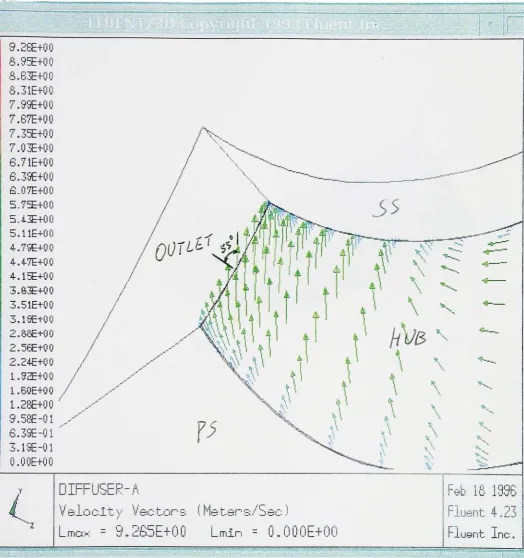
4.4A

Diffuser A:

Velocity

Vector

Plot

of

Slice J=2 (Near

Hub)

4.4B

Diffuser A: Zoom View

of

Velocity

Vector

Plot

at

Outlet

of

Slice

J=2 (Near

Hub)

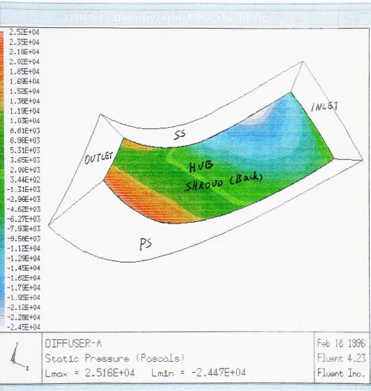
4.4C

Diffuser A:

Static Pressure

Distribution

Filled

Contour

of

Slice J=2 (Near

Hub)

4.

5 A

Diffuser A:

Velocity

Vector

Plot

of

Slice J=19 (Near

Shroud)

4.5B

Diffuser

A:

Static Pressure

Distribution

Filled Contour

of

Slice

J=19 (Near

Shroud)

4.6A

Diffuser

A:

Velocity

Vector

Plot

of

Slice

J=l 1

(Mid-Spanwise)

(10)

4.6B

Diffuser A:

Static Pressure Distribution Filled Contour

of

Slice J=l 1

(

Mid-Spanwise)

4.7A

Diffuser

A:

Velocity

Vector Plot

of

Slice

1=2

(Near

SS)

4.7B

Diffuser A:

Static

Pressure Distribution Filled Contour

of

Slice 1=2 (Near

SS)

4.8A

Diffuser A:

Velocity

Vector Plot

of

Slice 1=19 (Near

PS)

4.8B

Diffuser A:

Static

Pressure Distribution Filled Contour

of

Slice 1=19 (Near

PS)

4.9A

Diffuser A:

Velocity

Vector Plot

of

Slice 1=1

1

(Mid-Pitchwise)

4.9B

Diffuser A:

Static

of

Slice 1=1

1

(

Mid-Pitchwise)

4.10A Diffuser A:

Static

of

Slices

K=l,

30,

50, 70,

100

4.

1

1 A Diffuser

A:

Velocity

Vector Plot

of

Slice K=100

(Outlet)

4.1 IB

Diffuser A:

Velocity

Vector Plot

of

Slice

K=100

Side

View

(Outlet)

4.1 1C

Diffuser A:

of

K=l 00

(Outlet)

4.12A

Diffuser

B:

Velocity

Vector Plot

of

Slice J=2 (Near

Hub)

4.

12B

Diffuser

B: Zoom

View

of

Velocity

Vector Plot

at

Outlet

of

Slice J=2 (Near

Hub)

4.12C

Diffuser

B:

Static Pressure

Distribution

Filled Contour

of

Slice J=2 (Near

Hub)

4. 13

A

Diffuser

B:

Velocity

Vector Plot

of

Slice

J=19 (Near

Shroud)

4.13B

Diffuser

B:

Static Pressure

Distribution

Filled Contour

of

Slice J=19 (Near

Shroud)

4.14A Diffuser

B:

Velocity

Vector

Plot

of

Slice J=l

1

(Mid-Spanwise)

4.14B

Diffuser

B:

Static Pressure

Distribution

Filled Contour

of

Slice J=l 1

(

Mid-Spanwise)

4.15A

Diffuser

B:

Velocity

Vector

Plot

of

Slice 1=2 (Near

SS)

4. 1 5B

Diffuser

B:

Static Pressure

Distribution

Filled Contour

of

Slice

1=2 (Near

SS)

(11)

4. 16B

Diffuser

B:

Static Pressure Distribution

Filled

Contour

of

Slice 1=19 (Near

PS)

4.17A

Diffuser

B:

Velocity

Vector Plot

of

Slice

1=11

(Mid-Pitchwise)

4. 1

7B Diffuser B:

Static

Pressure

Distribution Filled Contour

of

Slice 1=1

1

(

Mid-Pitchwise)

4.18A Diffuser B.

Static

of

Slices

K=l, 30, 50, 70,

100

4.

19A

Diffuser

B:

Velocity

Vector Plot

of

Slice K=100

(Outlet)

4. 19B

Diffuser

B:

Velocity

Vector Plot

of

Slice

K=100 Side View

(Outlet)

4. 19C

Diffuser B:

of

K=100

(Outlet)

4.20A Diffuser C.

Velocity

Vector Plot

of

Slice J=2

(Near

Hub)

4.20B

Diffuser

C: Zoom View

of

Velocity

Vector Plot

at

Outlet

of

Slice

J=2 (Near

Hub)

4.20C

Diffuser

C: Static Pressure

Distribution

Filled Contour

of

Slice J=2 (Near

Hub)

4.21

A

Diffuser

C:

of

Slices

K=l, 30, 50, 70,

100

4.22A

Diffuser C:

Velocity

Vector

Plot

of

Slice K=100

(Outlet)

4.22B

Diffuser

C:

Velocity

Vector Plot

of

Slice K=100 Side View

(Outlet)

4.22C

Diffuser

C: Static Pressure

Distribution

Filled Contour

of

K=100

(Outlet)

4

23

Ideal

Diffuser Flow

Pattern

4.23 A

Velocity

Vector

Plot Comparison

of

Diffusers A.

B

& C

of

Slice J=2 (Near

Hub)

4.23B

Static

Pressure Distribution

Comparison

of

Diffusers

A,

B

& C

of

Slice J=2 (Near

Hub)

List

of

Tables

3

.

1

Model

Geometry

Comparison

4. 1

Summary

of

Results

4.2

Test Data for

Diffuser

A

& B

4.3

Comparison

of

CFD Results & Test Data

(12)

List

of

Symbols

Nomenclature

A

Net

Flow

Cross Area

AR

Area Ratio

C1.2

Empirical

Constants in

s and

k

equations

Cu

Empirical

Constant

in

Viscosity

Model

Cp

Pressure

Recovery

Coefficient

Cp.

i

Ideal Pressure

Recovery

Coefficient

E

Log

Law

Constant

G

Shear Generation Term

k

Turbulent

Kinetic

Energy

kr

Von

Karmans'

Constant

kP

Near Wall

Turbulent

Kinetic

Energy

/

Turbulence

Intensity

L

Diffuser

Wall Length

/

Turbulence

Length Scale

P

Fluid Pressure

P*

Dimensionless

Pressure

Q

Flow

Rate

[Gpm]

R

Radius

of streamline

Re

Reynolds

Number

(13)

t

Time

//

Friction

Velocity

//,

Velocity

in

i-direction

if

Dimensionless

Velocity

up

Near Wall

Velocity

I

'

Diffuser

Inlet Fluid

Velocity

I

'm

Meridional

Velocity

V

Normal

Velocity

(velocity

component

in

the

direction

of

diffuser

channel)

V,

Tangential

Velocity

(velocity

component orthogonalto the

direction

of

diffuser

channel)

W

Diffuser Width

Dimensionless Normal Distance from Wall

Greek Letters

i]

Diffuser

Efficiency; Arbitrary

Field

Variable

s

Dissipation

Rate

of

k

6

Divergence Angle

of

Diffuser

5

Boundary

Layer

Thickness

p

Fluid

Density

n

Pi [3.14159

...J

co

Vorticity

r

Shear Stress

(14)

a

Empirical

Constants

Oh

Turbulent

Prandtl Number

fj.

Absolute

Viscosity

Subscripts

I

Inlet Node

2

Outlet Node

/

Grid

Index

in

the

Spanwise Direction

J

Grid Index in

the

Pitchwise Direction

K

Grid Index in

the

Streamwise Direction

n

Normal

Direction

b

Binormal

Direction

s

Streamwise

Direction

(15)

Chapter 1 Introduction

1.1 Project Background

Diffusers

are one ofthe

basic

componentsof centrifugal

pump

systems.

The primary

function

ofa

diffuser is

to convert the

inlet

dynamic

pressure

(kinetic

energy)

to a static

pressure

rise.

For

subsonic

flow

this

is

done

by decelerating

the

fluid

particles

by

providing

a continuous and gradual

increase

ofthe cross-sectional

flow

area.

The desired

effect

is

to

recoveras much ofthe

inlet

dynamic

pressureaspossiblewith

steady flow

conditions.

The

scope ofthis thesis covers the analysis of a turbine-bowl

diffuser

used

in

a

mixed

flow

multi-stage

pump,

and to

investigate

the

applicability

of

using CFD

code as an

aid

in

designing

effective

diffusers.

The

multistage

pump has

a

15

inch

outside

bowl

diameter,

and the

pump has

a specific speed of

4750.

(Specific

speed

is

a

dimensionless

coefficient

for

compare certainaspects ofthe

different

families

of

turbomachines.)

In

order to

have

optimum performance, a mixed-flow

pump,

not

only

requires an

optimally designed impeller but

also a

matching designed diffuser.

Currently,

there are two

versions ofthe

diffuser:

Diffuser

A

and

Diffuser

B,

Diffuser B

was shaped

by

untwisting

Diffuser

A along

the

bowl

axis

approximately

five degrees.

1.2 Project Objectives

Present diffuser design

methods

lack

theoretical

depth

and sufficient empirical

data

for

determining

the optimum geometry.

This lack

of

knowledge is

in

part

due

to the

complexnature of

flow

in

diffusers,

and

is

also

due

to

the

difficulty

of

making

the required

(16)

The

project goal at

RIT

is

to

modify

a mixed

flow

pump's

diffuser geometry

to

improve

the

discharge

performance

by

using FLUENT

computational

fluid

dynamics

analysismethod.

The

task ofthis thesis wasto

develop

athree-dimensionalturbulent model

of current

designs

as

base

models,

then

modify

these

designs

for

improvements

using

FLUENT.

The

method of

increasing

the

diffuser

performance,

however

should not

significantly

alterthe

diffuser

geometry.

1.3 Project Description

All

centrifugal pumps utilize

but

one

pumping

principle: the

rotating impeller

imparts

energy

to

fluid,

building

up

a

velocity head.

At

the

periphery

ofthe

pump

casing.

the

fluid

is directed

into

a

diffuser.

The diffuser

most often

has

a

constantly

increasing

cross-sectional area

along

its

length,

so that as the

fluid

proceeds

along

the channel,

its

velocity

is

reduced.

Because

the

energy level

ofthe

fluid

cannot

be

substantially dissipated

atthis point, the conservation ofthe

energy

requiresthat whenthe

fluid

loses

kinetic

energy

as

it

moves

along

the channel,

it

must

increase

the

energy

related to pressure.

That

is,

the

pressureofthe

fluid increases.

A

mixed

flow

pump,

(a

type of centrifugal pump),

develops

head

partly

by

centrifugal

force

and

partly

by

the

lift

ofthe vanes on the

liquid.

This

type

of

pump has

a

single

inlet

impeller

with the

flow entering axially

and

discharging

in both

axial and radial

directions. Pumps

ofthis type

usually

have

aspecific speed

from 4200

to

9000.

(17)

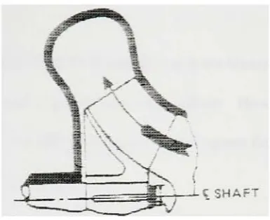
Figure

1

.

1

Mixed Flow

Pump

The

turbine-bowl

diffuser in

this thesis consists of eight passages which are

separated

by

eight vanes.

In

order to reduce computational effort, a three-dimensional

computational model

in FLUENT

was

developed for

one passageof each

diffuser design.

Based

on the

CFD

results

for Diffuser

A

and

B,

different

geometries were

constructed and modeled

in

order to

improve

the

design.

After

consultation with the

manufacturer, one ofthe modeled geometries was chosen and analyzed

in

this

thesis

as the

final improved design. This

is

labeled

as

Diffuser

C. The design

of

Diffuser C is actually

an

optimized

design

of

Diffusers A

and

B.

constructed

by

enlarging

the

intersecting

angle

between

suction side wall and outlet

in

the

hub from

90

to 108

This

modification

challenges the traditional

diffuser design

practice

in

the

industry

which

is

believed

that the

optimum

design

for

vane passageways to reduce

losses

is

a channel

that

is

as square as [image:17.554.185.378.60.217.2]

(18)

1.4 Literature Search

In

spite ofanextensive effort

for

literature

search via

library

and

Internet,

no article

was

found

relatedto thesubject ofmixed

flow pump diffuser.

However,

theresearch

relatedto mixed

flow

pump

and

diffuser

computer

modeling

and

flow

analysis was

insightful

which

is listed

as

following:

Zhang

and

Sun

(1995)

presented a method

based

ona

3-D

viscous

flow

analysis

for

theperformance prediction

for

themixed-flow

pump1

Favre

(1995)

introduced

a

full 3-D flow modeling

methodto

study

themixed-flow

pump impeller

performance2

Zhang

and

Garon

(1993)

presented a

3-D

simulation ofthepassage-averaged

vorticity-potential

formulation

ofthe

incompressible

viscous

flow

field

withina

mixed-flow

********

(19)

Chapter

2 Turbulent Flow

Theory

2.1

Governing

Equations

Turbulence4

is

one ofthe most

difficult

phenomena

in

the area ofphysical sciences.

In

turbulent

flow

situations,

the

fluid

motion

is

highly

random,

unsteady,

and

three-dimensional. Due

to

these complexities,

the turbulent motion and mass-transfer phenomena

associated with

it

are

extremely difficult

to

describe

and thus predict theoretically.

It

is

believed

that thesolution ofthe time-dependentthree-dimensional

Navies-Stokes

equations^

can

completely

describe

turbulent

flows.

This

can

be done

by

describing

the

fluid flow

at

every

point

in

the

flow

regime

for

all time

by

taking

into

consideration the principles of

conservation of

mass,

momentum and energy.

These

general equations

completely describe

the

fluid

flow (the

equation

for energy

conservation

is disregarded here due

to

its

irrelevance

totheproblem).

The

nature ofthe specific

flow

under consideration allows

for

some simplification.

It

is

assumed that within the

diffuser.

the

flow

can

be

described

as

turbulent,

steady,

incompressible, isothermal,

and

Newtonian in

nature.

The

conservation of

energy

equation

is

disregarded based

upon these assumptions, and the equations

for

conservation of mass

and momentumarereduced to:

(Eq.

1)

(Eq.

2)

^

=

₀

p

cP

c

d

[atl

{ex

(20)

where Uj

is

the

fluid

velocity

with

i, j

=

1

,

2,

& 3 for

athree-dimensional

problem, P

is

the

pressure,

and

F

represents

body

forces.

Ul

Methodology

of

Analysis

To practically

describe

turbulent motion,

it

is necessary

to use time averaged

quantities rather than

instantaneous

ones.

This

approach

is based

upon the conservation

laws for

mass and momentum

(Eq.

1

and

2). Osborne Reynolds

was the

first

to suggest

using

a statistical approach where the equations are averaged over a time scale which

is

comparatively

long

with that ofthe turbulent event

in

question.

The resulting

equations

describe

the

distribution

ofthemean

velocity

andpressure within thecontrol

volume^

In

this statistical _approach, each ofthe

field

variables

(velocity,

//;& _pressure,

P

)

are

separated

into

mean and

fluctuating

quantities which allows

for

the use of mean values of

the

field

variables

{it.

&

P)

in modeling

the

large

scale

flow

characteristics.

For

an

arbitrary field

variable

(r\),

themean value can

be defined

as

_

1

f'-v'

rj

=}tjc/C

(Eq.

3)

where the

averaging

time

At

is

long

compared with the time scale ofthe turbulent motion.

The instantaneous

variable

r\

is

then given

by,

rj

= ff+rj'

(Eq.

4)

where rf

is

the timeaveraged

quantity

and

if

reflectsthe small scale

fluctuations

associated

with turbulence.

This

decomposition

is

applied to the

Navies-Stokes

equations which are

then

integrated

over the time

interval

(t,

t +

At)

resulting in

the

following

time averaged

(21)

Due

to the

non-linearity

of

the

Navies-

Stokes

equations,

_the

averaging

process

introduces

a correlation

between

fluctuating,

velocities utu .

Multiplying

this term

by

p

givesthe transport ofmomentum

due

to the turbulentmotion.

The

relation

r

r-f

P",uj

=

J

pu;u;dr

(Eq.

5)

describes

the transport of_x; momentum

in

the

direction

of

Xj,

and acts as a stress on the

fluid

(Reynolds

stress).

It

summarizes the effect of small scale

eddy behavior

on the

large

scale mean

flow.

To

solve the

Navies-Stokes

equations and

Eq.

5

requires a

way

of

determining

the turbulence correlation.

This determination is

the main roadblock

in

analyzing

turbulent

flows.

A

turbulence model which approximates this correlation

along

with the Navies-

Stokes

equations

forms

a closed set of equations which can

be

solved

for

themean values of

velocity

and pressure.

Generally,

the two equation

k-s

turbulence model

is

employed to

facilitate

the

solution, where

k

stands

for

turbulent

kinetic energy

and s stands

for dissipation

rate.

In

the

k-s

model,

Reynolds

stressesare relatedto themean

flow

viathe

Boussinesq

hypothesis:

~> '

a,

at"

">

at

v<

J ex,

1

The

effective or

"turbulent"

viscosity, jut,

is

computed

from

a

velocity

scale (k2

)

and a

k2

length

scale

(

)

which are predicted at each point

in

the

flow

via solution oftransport

s

(22)

l{pk)

+

--(p,i,k)

=-?-l^--Gk+G>-pe

(Eq.

7)

a

exi

cxi

at.

exi

and

(Eq.

8)

c i , c , , c u. ce s

s2

"Tl

pe)

+

pu,e)

=~

'--L\pGk

-C\p

a

c*,

ex,

<j

ex

k

where

Gjk

is

thegeneration of

k

and

is

given

by:

(&',

ai\ai,

G,

=Mi\-~L\-(Eq.

9)

\

cx:

ex

j

ex

and

Gh

is

thegeneration

due

to the

buoyancy:

Gfc=-g,

-^

(Eq.

10)

poh

ex,

P,Cr

whereoi, isthe turbulent

Prandtl number,

k,

The

turbulent

viscosity is

thenrelatedto

k

and s

by

theexpression:

X-2

M,=PCU

(Eq.

11)

e

The

coefficients

C\, C2, Cib

ol,

and az are empirical constants which

have

the

following

empirically derived

values.

C,

=

1

.44,

C2

=

1

.92,

Q

=

0.09,

ak=\.0,ae=\.3

In

turbulent

flow,

the wall

boundary

layer

consists ofa

laminar

sublayer and a

so-called

log-law

region

in

which the

flow

is

fully

turbulent.

In

the

log-law

region, the

wall

(23)

".

1

-4=

ln(>'")

(Eq.

12)

where

v

=

Von

Karmans'

constant

(0.42)

E

=

log

law

constant

(9.8)

u =

friction

velocity

-V

P

tip=

near wall

velocity

Note

that the assumption of equilibrium

in

the

boundary

layer (production

equal to

dissipation)

can

be

used to

derive

the

following

expression

for

v

(dimensionless

normal

distance

from

wall):

v

^^

IV 1^

>' ₌

(Eq.

1j)

M

where:

kv

=

near wallturbulent

kinetic energy

p

=

fluid viscosity

A>> =

distance

to thewall

In

general, the

inlet

turbulence

intensity

and characteristic

length

are a

function

of

the

flow

parameters upstream.

The

turbulence

intensity

is defined

as the ratio of

the

turbulent

fluctuations in

velocity

to the mean

flow velocity (

'

/

avg),

expressed as a

percentage.

The

inlet

values of

k

and s are calculated

from

the specified

inlet

turbulence

(24)

0.2

Core

-Flow

(TV)

1

yA

/

I

/

Fully

Turbulent Flow

0.1

Fully

Turbulent Layer

(IH)

Buffer

Wall Layer

Layer

(D)

Viscous Sublayer

(1)

y,/R

1

A-x-~^~~^

i

Viscoa Layer

777?MV//V^^ '//////////////////////////..

1

[image:24.554.92.466.208.511.2]

(25)

or

k

=

^(u^l)2

(Eq.

14)

The

dissipation

rate

is

thengiven

by:

e=CJ^-

(Eq.

15)

where

/

is

a

length

scale characteristicofthe turbulence

in

the

inlet

flow.

The

characteristic

length

is

used to computethe

mixing length for

the small-scale eddies and should

be

set to

the

hydraulic

radius ofthe

inlet.

The

inlet

turbulence

length

scale,

/,

is

calculated

by:

/

=

0.077?

(Eq.

16)

Note

that the

factor

of

0.07

is derived from

the"average"

mixing length in

turbulent pipe

flow,

where

R

is

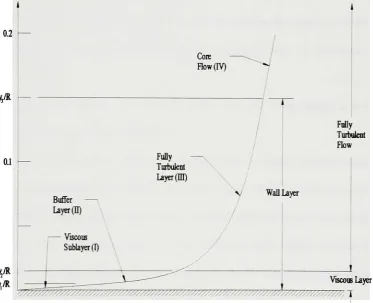
theradius ofthepipe.

The

turbulent

flow

regime can

be described

by

distinct

regions

based

upon the

definitions

and characteristics

from

above.

The

viscous sublayer

is

theregion nearestto the

wall where

is less

thanor equal to

five.

The

fully

turbulent core

is

nearthe centerlineof

the

flow

where v

is

greater than

30.

The buffer

region

is

located between

the viscous

sublayerand the

fully

turbulentregion.

Figure 2. 1

showsthese regions

in

a graphical

form.

The

regions are

defined

by

the

different flow

characteristics that are

found

within each

region,

which

is helpful in

discussing

thecomplexities ofturbulent

flow.

2.3 Diffuser Flow

One

ofthe

basic

components ofa

pump

is

the

diffuser.

The

diffuser's purpose

is

to

convertthe

inlet dynamic

pressure ofthe

fluid

to a static pressure rise.

For

subsonic

flow,

this

is

accomplished

by decelerating

the

fluid

particles

by

the application of a gradual

(26)

[image:26.554.72.485.100.612.2]

(27)

increase

ofthecrosssectional

flow

area.

It

is desirable

to recoveras much ofthe

entering

dynamic

pressure as possible.

It

is

also

important

that the

exiting flow

be

steady

and

has

a

uniformprofile

for

thenext

impeller

stage.

There

are several parameters used to

describe

a

diffuser

geometry6

These

quantities are useful

in analyzing

the performance ofthe

diffuser.

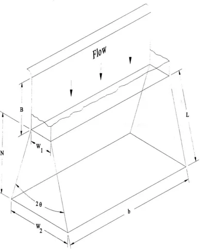
A

simple

flat diffuser is

shown

in Figure 2.2.

The geometry

ofa

diffuser

is

specified

by

the aspect ratio

b/Wi,

the

divergence

angle

20,

the

length-to-width

ratio

L

Wi,

and the cross-sectional area ratio

W2

W\.

The

pressure

recovery

coefficient

Cp

describes

theperformanceofa

diffuser:

CP=~r

L

(Eq.

17)

where

P2

is

the outlet static

pressure,

Pi

is

the

inlet

static

pressure,

and v,

is

the throat

velocity.

Under

ideal

conditions,

the maximum pressure

recovery

coefficient

Cp.ideai

is

a

function

ofthe

geometry

and

is

given

by

where

AR

is

the area ratio.

The

ratiooftheactual pressure

recovery

coefficientto the

ideal

pressure

recovery

coefficient

is known

asthe

diffuser efficiency

77.

rj=

(Eq.

19)

(

_{P. Ideal}

In

the

diffuser,

the

development

ofthe turbulent

boundary

layer has

a significant

impact

on the

diffuser

performance.

If

the turbulent

boundary

layer

is

thick enough to

create a

large

throat

blockage,

separation will occur nearthe

inlet

ofthe

diverging

section.

(28)

The

fluid

particles

decelerate

near thewall regionundertheeffect of an

increasing

pressure

gradient and reduced transverse momentum transfer.

As

the

fluid

progresses through the

diffuser,

in

the presence of

flow

separation,

excessive

blockage

occurs,

which

in

turn

reducesthe

diffuser

efficiency.

2.4

Secondary

Flows

Due

to the

diffuser

wall

3-D

curvature,

secondary

flows

can

be easily found in

a

mixed-flow

pump

diffuser.

The

cause of

secondary

flows

can

be

traced to the

dynamics

of

streamwise

vorticity,

with reference to a right-hand reference system composed of

streamwise

(s),

normal

(),

and

binormal(A)

directions.

Under

the

hypotheses

of

incompressible stationary

flow,

theproductionof streamwise

vorticity is:

cfcoA

2co

cs\\

J

Rv

where co

is

vorticity,

v

is

absolute_velocity, and

R

is

radius of streamline.

Eq. 20

can

be

reduced

by

use ofthe

Bernoulli's

equation and scalar product

in direction b

to:

c VN

2

cv

2

cPt

csVpvJ

(Eq.

21)

Rpv

ab

Rpv' cb

where

P,

stands

for

totalpressure.

The

production of streamwise

vorticity

depends

thus

on the gradients of

velocity in

binormal direction.

These

gradients of

velocity

are

typically

associatedwiththepresence of

boundary

layers,

which are encountered on the

hub

and shroud walls as well as on the

suction and pressure side walls.

It

is

possible to separate

the

effects ofshroud

to

hub

and

pressureto suctionsidewall curvatures:

(29)

a)

Shroud

to

Hub

Curvature

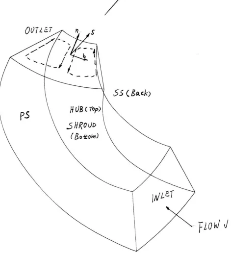
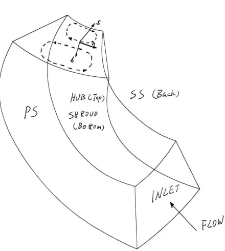
Figure 2.3

is

a schematic ofthe mixed

flow

pump

diffuser,

the normal n points

inward

in

radial

direction,

that

is

from

shroud to

hub;

the

binormal b

is

in

tangential

direction

from

pressure side

(PS)

to suction side

(SS).

Under

these

conditions,

{cTtld))

is

positive on

PS (total

pressure

is increased

at the outer

PS

boundary

layer),

and negative on the

SS

(total

pressure

is decreased

at the

inner SS

boundary

layer).

Vorticity

production

(clockwise;

displacing

n towards

b)

is

positive on

PS

and negative

(counterclockwise,

displacing

b

towards

)

on

SS.

This

means that the

direction

of

secondary

flows

will

be from

shroud to

hub both

on

both PS

and

SS

wall

surface:

low-total

pressure

fluid

accumulates

in

the

hub

boundary

layer

and thenrecirculates

to the shroud at the center ofthe

diffuser

passage.

This

pattern,

shown

by

dashed

lines

in

Figure 2.3

is

responsible

for

the rapid

buildup

ofa

large hub

boundary

layer,

which

is

then

subject to

further secondary

effects.

b)

PS

to

SS

For

PS

to

SS

curvature

(Figure

2.4),

the normal n

is

directed

in

tangential

direction

from PS

to

SS;

the

binormal

b

points outward

in

radial

direction,

that

is

from

hub

to shroud.

Under

these conditions.

{cPtlcb)

is

positive at the

hub (total

pressure

is

increased

at the outer

hub

boundary

layer),

and negative at the shroud

(total

pressure

is

decreased

at the

inner

shroud

boundary

layer).

Vorticity

production

(clockwise,

displacing

n towards

b)

is

positive at the

hub

and negative

(counterclockwise;

displacing

b

towards n)

atthe shroud.

This

would meanthat

secondary

flows

should circulate

from PS

to

SS

at

the

both

hub

and shroud

(dashed lines in Figure 2.4).

(30)

Flow

Oonz<

\

.s

SSifath

J

10

hi

J

[image:30.554.47.519.61.578.2]

(31)

Flow

[image:31.554.59.500.88.579.2]

55

(3**-)

(32)

Chapter

3

FLUENT

Description

and

Implementation

3.1

FLUENT

CFD

code

introduction

3.1.1 Code

Application

and

Features

The

use of advanced computational

fluid

dynamics

techniques

is very helpful in

the

analysis of complex

flow

patterns encountered within a centrifugal pump's sub

components.

In

this work

FLUENT

was used

for

such a purpose.

FLUENT

is

a general

purpose computational program

for modeling

fluid

flow,

heat

transfer,

and chemical

reactions.

FLUENT

models this wide range of phenomena

by

solving

the conservation

equations

for

mass, momentum, energy, and chemical species

using

a control volume

based

finite-difference

method.

The governing

equations are

discretized

on a curvilinear grid to

enable computations

in

complex/irregular geometries.

A

nonstaggered system

is

used

for

storageof

discrete

velocities and nodal pressures.

Interpolation

is

accomplishedvia a

first-order,

Power-Law

scheme or

optionally

via the

higher

order

QUICK

scheme.

The

equations are solved

using

the

SIMPLEC

algorithm with an

iterative line-by-line

matrix

solverand multigrid acceleration or withthe

GMRES

full-field

iterative

solver7

In

this thesis

work,

FLUENT

was used to analyze regions of

stagnation,

flow

separation,

and

secondary flow

patterns within the various

diffuser

configurations.

The

flow

was modeled

in

three

dimensions

and accounted

for

the

incompressibility

and viscous

nature ofthe

flow.

FLUENT

presents several options

for

the solution ofthe

Reynolds

averaged Navier-

Stokes

equations

for

turbulent

flow.

This

solution

incorporates

the

two-equation

kinetic energy dissipation

turbulence

k-s

model.

In

this

turbulence

model,

the

(33)

turbulence

field

is

characterized

in

termsof

two variables,

the turbulent

kinetic

energy,

and

the viscous

dissipation

rate of

kinetic

energy.

The

criteria

for effectively using

finite

difference

method are numerous

in

order

to

ensure a solution that converges and gives

realistic results.

Among

the most

important

are the choices ofgrid

density

and cell

types,

inlet

and

boundary

conditions,

solution

techniques,

andtheextension ofthe

kinetic

energy-dissipation

modelto thenear-wall region.

3.1.2 Program

Structure

FLUENT

is

atwo part program

consisting

of a preprocessor

-PreBFC,

and a main

module

FLUENT.

PreBFC

is

used to

define

the

geometry

and a structured grid

for

the

model.

Then

thegrid

information is

transferred

from PreBFC

to

FLUENT

via a

GRID File.

Following

this

transfer,

FLUENT

is

used to

define

physical models,

fluid/material

properties,

and

boundary

conditionsthat

describe

theproblem.

This

information is

addedto

the grid

information

and stored

in

a

Case File

that

is

a record ofall the

inputs

for

problem

definition.

Calculation

and

post-processing

are also performed

in

FLUENT,

the results are

stored

in

a

Data File.

3.1.3

Modeling

Technique

3. 1.

3.

J Problem

Solving

Steps

Once

the

important features

ofthe problem are

determined,

the

basic

procedural

steps arethoseshown

below:

1

.

Create

or

import

themodel

geometry

and grid.

2.

Choose

the

basic

equations to

be

solved

(i.e.

enthalpy,

species,

turbulence

transport).

(34)

3.

Identify

additional models needed

(fans,

porous

media,

special

boundary

conditions,

speciestransportor chemical

reaction,

etc.).

4.

Specify

the

boundary

conditions.

5.

Specify

the

fluid

properties

6.

Set

up

a

dispersed

phase

(optional).

7.

Adjust

the solution controlparameters

(optional).

8.

Calculate

asolution

(fluid

phaseand/or

dispersed

phase).

9.

Examine

theresults.

10.

Save

theresults.

1 1

.

Consider

revisionsto the numerical or physical model.

3.1.3.2

Choosing

a

Suitable Grid

The

grid represents a

discrete

approximation ofthe continuous

field

phenomena

that users must model.

The accuracy

and numerical

stability

ofthe

FLUENT

calculations

depend

onthesegrid characteristics.

In

otherwords, the

density

and

distribution

ofthegrid

lines determines

the

accuracy

with which the

FLUENT

model representsthe actual physical

phenomena.

In

FLUENT,

the control volume

method,

sometimes referred toas the

finite

volume

method,

is

used to

discretize

the transportequations.

In

the

discrete

form

of

the equations,

values of the

dependent

variables appear at control volume

boundary

locations.

These

values

have

to

be

expressed

in

terms of

the

values at thenodes of

neighboring

cells

in

order

to obtain solvable algebraic equations.

This

task

is

accomplished via an

interpolation

(35)

practice

known

as a

"differencing

scheme"

The

choice of

differencing

scheme not

only

affectsthe

accuracy

ofthesolution

but

the

stability

ofthenumerical method.

3.1.3.2.1 Grid

Spacing

near

Walls

In

turbulent

flow,

the

spacing

between

the wall and the adjacent grid

line

should

be

suchthat the grid

line lies

in

the

log-law layer

oftheturbulent

boundary

layer.

This

implies

a

dimensionless distance from

the

wall, y~,

greater than about

25

and

less

than about

300-500.

3.1.3.2.2

Non-Uniform Grid

Spacing

One

way

to minimize the number ofcells while

maintaining

a sufficient

degree

of

accuracy in

the solution

is

to use a non-uniform grid.

In

a non-uniform

grid,

the grid

spacing

is

reduced

in

regions where

high

gradientsare expected and

increased

in

regions

wherethe

flow is relatively

uniform.

The

rateofchange ofgrid

spacing

should

be

minimized

due

to stability effects that

result.

Normally

the

spacing between

adjacent grid

lines

should not change

by

more than

20%

or

30% from

onegrid

line

to thenext which

implies

expansion

factors

between

0.7

and

1.3.

This is

an

accuracy

consideration,

primarily

impacting

the

accuracy

ofthe

diffusion

terms

in

the

governing

transportequations.

3. 1. 3. 2. 3 Cell Aspect Rations

The

aspect ratio ofthe computational cells

is

an additional

issue

that arises

during

the

setup

ofthe computational grid.

While

large

aspect ratios

may

introduce

acceptable

degrees

of error

in

some

problems,

ageneral ruleofthumb might

be

to

avoid aspect ratios

in

excess of

5:1.

This

limit

can

be

exceeded without significant consequence when

the

(36)

gradients

in

one

direction

are

very

small relative to those

in

the second

direction.

Conversely,

excessive aspect ratios can

lead

to

stability

problems,

convergence

difficulties,

andthepropagationof numerical errors.

3.1.3.2.4

Grid

Skewness

When using

body-fitted

coordinates,

the grid

lines may

not

be

orthogonal.

While

some

degree

of

nonorthogonality is

allowable, and

is

accounted

for in

the solution

process,

the computational grid should maintain grid

intersection

angles close to

90

degrees

wheneverpossible.

3.1.3.2.5

Weighting

Factors for Grid Redistribution

Weighting

factors

can

be

used to control the grid

density

at each endpoint of a

segment.

A weighting factor

greaterthan

1.0

implies

thatthegrid

density

will

be

increased,

thusa

finer

(denser)

grid attheendpoint can

easily be

achieved

3.1.3.3

Solver Selection

The default

k-s

model

is

a semi-empirical model that

has been

proven to provide

engineering accuracy in

a wide

variety

ofturbulent

flows

including

flows

with planar shear

layers

such as

jet-flows,

duct

flows,

etc.

This

model was

found

suitable

for

the conditions

present

in

this project.

3.2

Diffuser

Modeling

Process:

Since

the

flow

pattern

in

each

diffuser

channel

is

identical,

only

one channel was

modeled

in

each ofthe three

diffuser designs.

3.2.1

Geometry

Creation:

(37)

The geometry data for Diffuser

A,

R

and

C

is

given

in Table 3.1.

This

table

providestheaxial

(Z)

, radial

(R),

and chord angle

(

9)

coordinates

for

the points

along

the

two

sides ofone oftheeight

blades

in

the

diffuser:

The inner

side

is

the

intersection

of

SS

and the

hub

side,

andthe outer side

is

the

intersection

of

SS

and the shroud side.

Chordal

thickness

(

Th)

of

inner

&

outer side represents the

diffuser PS

and

SS

wall thickness.

All

the

data

was supplied

in English

units,

thusgeometries were constructed

in English

units

in

Cadkey

and

PreBFC

and converted

into SI

units

in FLUENT.

Figure 3.1

shows the

diagram

ofthe

diffuser location

inside

a mixed

flow

pump.

To

reducethecomputationaland analysis effort,

it

was criticalto

find

and

locate

the

inlet

and outlet planenormal to the

diffuser

channel.

This

became

one ofthe most

difficult

challenges

due

to the diffuser's complex geometry.

Finding

these planes exceeded the

capability

ofthe

PreBFC

package,

which constructs

geometry only based

on coordinates.

Cadkey

3-D

software was

introduced into

theproject to

find

the normal planes.

The

raw

geometries were

built

up

based

on

geometry

data,

and then the normal

inlet

and outlet

planes were

located using

the

recently introduced

surface package offered

in

Cadkey

version

7

The

excess portion ofthe

geometry

was removed

from

the model

along

the

normal

inlet

and outletplanes.

The resulting diffuser

channel point coordinates were

input

into

the

PreBFC

to generatethe

CFD

models.

Diffuser

A:

This

wasthe original

design.

As

shown

in

Figure

3.5,

from

outlet to

inlet:

the

twisting

angle ofthe

PS

and

SS

walls on the

hub

side ranged

from

0

to

62.36

degrees,

onthe shroud side

increased from 3.35

to

77

degrees;

the

hub

radius varied

from

1

.912

in

to

4.875

in,

while theshroud radius varied

from 4.909

in

to

7.026 in

(38)

Table 3.1

Model

Geometry

Comparison

Diffuser A

InnerSide Blade OuterSide Blade

# Axial Radial Chord Angle Chord Thickness Axial Radial Chord Angle Chord Thickness

(to)

(degree)

(to)

(degree)

(to)

1 12.507 1.912 0 0.125 14.035 4.909 3.35 0.218

2 11.864 2.451 1 0.138 12.879 5.475 4.35 0.295

3 10.866 3.288 10 0.182 11.867 6.055 10 0.39

4 10.2 3.847 20 0.223 10.806 6.539 20 0.47

5 9.526 4.359 30 0.254 9.787 6.858 30 0.479

6 8.786 4.699 40 0.238 8.725 7.056 40 0.491

7 8.042 4.857 50 0.227 7.672 7.125 50 0.477

8 7.21 4.875 62.36 0.22 6.347 7.125 62.36 0.432

9 5.059 7.026 77 0.333

Diffuser B

Inner Side Blade Outer Side Blade

# Axial Radial Chord Angle Chord Thickness Axial Radial Chord Angle Chord Thickness

1

(to)

12.507

(to)

1.9118

(degree)

0

(to)

0.125

(in)

14.035

(in)

4.909

(degree)

0

(to)

0.1875

2 11.647 2.6335 1 0.245 12.5411 5.6706 1 0.5

3 10.9983 3.1779 5 0.255 1 1.2989 6.3345 5 0.55

4 10.4526 3.6358 10 0.2416 10.5518 6.6308 10 0.543

5 9.6504 4.2799 20 0.2395 9.4302 6.9391 20 0.458

6 8.8753 4.6682 30 0.244 8.353 7.0943 30 0.3632

7 8.1631 4.842 40 0.2472 7.3604 7.125 40 0.3908

8 7.5531 4.875 50 0.2502 6.455 7.125 50 0.4121

9 7.1773 4.875 57.1889 0.2534 5.8621 7.1124 57.1889 0.433

10 5.059 7.0264 67.9884 0.3807

Diffuser

C

Inner Side Blade Outer Side Blade

# Axial Radial Chord Angle ChordThickness Axial Radial Chord Angle ChordThickness

(to)

(degree)

(to)

(degree)

(to)

1 12.507 1.9118 -9.2436 0.125 14.035 4.909 0 0.1875

2 11.9707 2.3619 -5 0.1367 12.5411 5.6706 1 0.5

3 11.3719 2.8644 0 0.1525 11.2989 6.3345 5 0.55

4 10.8591 3.2947 5 0.1853 10.5518 6.6308 10 0.543

5 10.4273 3.657 10 0.2219 9.4302 6.9391 20 0.458

6 9.6503 4.28 20 0.2395 8.353 7.0943 30 0.3632

7 8.8753 4.6682 30 0.244 7.3604 7.125 40 0.3908

8 8.1631 4.842 40 0.2472 6.455 7.125 50 0.4121

9 7.5531 4.875 50 0.2503 5.8621 7.1124 57.1889 0.433

(39)

iJBSll^s

Ei

s s

j 5

=

3

1

8

C o

'a

u

o

h4 Ui u

Q

Cm

O

u (75

(40)

Diffuser

B.

This

was an

improved

design

developed

purely

by

experience,

no

CFD

analysiswas

done

on

Diffuser B

prior to this thesis work.

As

shown

in Figure

3.5,

from

outletto

inlet:

the

twisting

angleofthe

PS

and

SS

wallsonthe

hub

sideranged

from 0

to

57.

19

degrees,

onthe shroud side

increased from

0

to

67.98

degrees;

the

hub

radiusvaried

from 1

.9

12 in

to

4.875

in,

whilethe shroud radiusvaried

from 4.909 in

to

7.026

in.

Diffuser

C:

Diffuser C

is

an optimized

design combining

aspects of

Diffuser A

and

B.

As

shown

in

Figure

3.6,

Diffuser

C has

an

enlarged,

108

vs.

90,

intersecting

angle

between

SS

and outlet

in

the

hub.

As

shown

in Figure

3.5,

from

outlet to

inlet:

the

twisting

angle ofthe

PS

and

SS

walls onthe

hub

sidewas

increased from

-9.24 to

57.

19

degrees,

on

the shroud side ranged

from

0

to

67.98

degrees;

the

hub

radius varied

from 1.912 in

to

4.875

in,

andtheshroud radiusvaried

from 4.909 in

to

7.026

in.

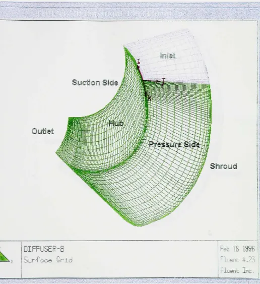
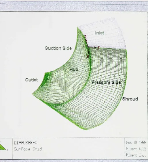
3.2.2 Grid Generation:

The

grid

density

is

the most

important

criteria

for providing

a realistic and

converging

solution.

In

order to obtain the optimal grid

density,

many

parameters ofthe

region

had

to

be

taken

into

consideration.

This

was accomplished through trial-and-error.

A

Body-Fitted

Coordinate Based

grid withacurve segmentation size of

I

=

20. J

=

20

and

K

=

100

(total 44541

cells)

was chosen

for

themodel.

As

shown

in Figure

3.2,

I

is

taken

along

the pitchwise

(PS

to

SS) direction,

J

is

taken

along

spanwise

(hub

to

shroud)

direction,

and

K

is

taken

along

streamwise

(inlet

to

outlet)

direction.

(The

grid selection

is

the same

for Diffuser B

and

Diffuser

C

as shown

in Figure 3.3

and

Figure

3.4.)

The 20

x

20

x

100

grid provided adequate resolution and the value of was

approximately

40

at

grid points adjacent to the

PS

and

SS

walls.

The

value of

y

was

approximately

45

at grid

(41)

points adjacent to

the

shroud and

hub

surfaceswhich ensured

the

grid

line

to

lie in

the

log-law layer

of

the turbulent

boundary

layer

as

discussed in

paragraph

3.1.3 2

1

-

Grid

Spacing

near

Walls. The

major steps

involved

in generating

thegridare as

follows:

1

.

Specify

the node

distribution along

the

boundaries

(map

the

boundaries).

2.

Adjust

themapped nodes

along

the

boundaries.

3

.

Create

thegrid

inside

the

domain

via

interpolation.

4.

Smooth

the

interpolated

grid.

5.

Display

and

verify

thegrid.

It

was

determined

that the grid needed to

be finer

in

regions where properties of

interest

were

changing

rapidly.

It

was also

important

to notethat care must

be

exercised

in

the

design

ofthecomputational meshtoensure asmooth spatial

distribution

of nodal points

throughout the entire

flow domain.

If

the transition

in

grid

density

was _abrupt,

especially

along

the

direction

of

flow,

spurious spatial oscillation

in

the

flow

variables

may be

observed

causing

a

divergent

numerical solution.

Since

the

majority

of

losses,

flow

separationandvortices occur nearthe

walls,

dense

cell

layers

should

be

set close to walls to catch those phenomena.

In

other words, to

effectively

capture viscouseffects,grids areclustered near wall surfaces.

This

can

be done

by

redistributing

nodes

according

to specified

weighting

factors.

Dividing

the

distance between

nodes

in

theneighborhood ofthe selected adjustment points

by

the

weighting

factor

will redistributethe nodes

according

to a smooth

hyperbolic

tangent

function.

The

following

grid

weighting

factors

are

found

suitable

for

the

diffuser

model:

(42)

Outlet

i

j;

if

f

^.

DIFFUSER-jiun oce

brid

I

Feb

18

1356

j

Fluent

423

i

hlusnt

Inc

.

(43)

Outlet

Suction Side

M

I

1

I

urr

5ER-B

SijrT

OC

Irf

'Id

Feb 16 139

F

Luent

4.2/

Fluent

lnc

:

[image:43.554.24.541.69.633.2]

(44)

j

t

-I

!

I

II >_!_

JSE

P4-. Ifl JQQC

burr

qc Hi!l

iT-FluBnt

ire:.

[image:44.554.22.537.71.633.2]

i '".;

..._._.._,____,. ,

(45)

o

c

a

o

g>

IP

<

o _a

too a a

c/3

CO

CQ

(46)

<

c

o

3

C O on in

$s

3

o

e <u <u

PQ jy

00

c

<

c '-4'

o

0)

Q

CO <D ' 3

(47)

Hub(Jl)

PS

(II)

Shroud(J20)

SS(I20)

Inlet:

10-10

Outlet: 10-10

10-10

A

grid

weighting factor

of

3

-

3

was also applied

along

the channel

from inlet

to

outlet to account

for any

flow

pattern change

in

the

inlet

and outlet region.

Six-point

interpolation

method was used

for

grid generation.

A

grid verification

is

performed after

the grid

generation,

which

includes

cell

type check,

cell volume

check,

relative cell size

check and skewness check.

The

models passed all the standard check requirements which

are the program

defaults:

20

to

1

ratio of maximum volume ratio

between

adjacent

cells,

and

60

degrees

maximum

deviation from

orthogonal.

%%.%.%.%5 %;%

This

area

intentionally

left

blank.

********

(48)

3.2.3

Case File Generation

(Boundary Conditions

and

Assumptions):

In

this phase of

the modeling,

constraints and variables such as geometric unit

conversion,

fluid

properties,

and

boundary

conditionswereapplied

to

the model.

For

this

problemthe

SI

system wasthe unit

base

chosen

for

analysis.

Water

was used asthe

fluid

medium with

density

=

1000

kg/m\

and absolute

viscosity

=

9.8

x 10""1

kg.s/m

at

20

C.

The

modulechosen

in

FLUENT only

required the

inlet

boundary

conditionto

fully

define

themodel.

The

no

slip

condition onthewallsurfaceswasalso

input

into

theprogram.

In

order to predict

flow

patterns

for

the

inlet

boundary

conditions at the

design

flow

rate,

normal velocities toward the

inlet

plane are adopted since the

incidence

angle

effects were unknown.

The

normal

velocity

was calculated

based

on

4500

gpm

flow

rate:

rr

Q

4500?/w7x 3.7854

x

10''m3

1

gallon ..,., ,. ,

V

= =

^ ; =_?

16.8 \m

I

_min=

8.6 \m

I

_sec "

A

8x412x1(T3ot-For

each channelthe

inlet

surfaceareawas

4.

12x10""' m2

pvD 1

000A-? /

m

:"

8.6 \mIs 0.064;/;

Re=

-= : =₅₆₂₂₉

H 9.8x10

^kg.s/m

Given

this

high Reynolds

number,

it is

clear that turbulent

flow

is

present within

the

diffuser.

The

k-s

turbulent

flow

model was

used,

which requires

inlet

turbulence

intensity

and characteristic

length input.

A

turbulence

intensity

of

10%

(based

on the

design flow

of

4000

to

5000 gpm),

characteristic

length

of

0.032

m were used as

inlet

condition.

Due

to the adiabatic nature ofthe

diffuser,

isothermal

flow

conditions were

(49)

3.2.4

Computine

The Results:

For

each

model,

approximately

1000

iterations

were performed to reach the

FLUENT

default

convergence criteria.

The

programmed criteria proved adequate

for

this

study

and

did

not require alteration.

Data

files

were created

during

the program analysis

which contained the solution

for

the

CFD

problem.

Results

were presented

in both

graphical

(velocity

vector

plot,

pressure

distribution

contour

plot)

and numerical

format.

********

This

area

intentionanv

ieft blank.

********

(50)

Chapter

4

Results &

Discussion

4.1 General CFD Results

4.1.1

Alphanumeric

Illustration

The

goal of a

diffuser is

to convertthe

inlet

dynamic

pressure ofthe

fluid

to a static

pressure rise.

It

is desirable

to recoveras much ofthe

entering dynamic

pressure aspossible.

It

is

also

important

that the

exiting flow be steady

and

has

a uniform profile

for

the next

impeller

stage.

Table 4.

1

lists

thegeneral results

from

the

FLUENT

program

for Diffusers

A,

B

and

C

Table

4.

1

-Summary

of

Results

AR

Static

Pressure

Recovery

AP

(Pa)

cP

Cp,

ideal

Diffuser

Efficiency

Diffuser A

1.303

7745

0.209

0.41

50.90%

Diffuser B

1.406 13415

0.303

0.49 61.33%

Diffuser C 1.426 14202

0.330

0.51

65.03%

Compared

with

Diffuser

A,

Diffuser B

has approximately

an

8%

area ratio

increase,

the static pressure

recovery

coefficient,

CP,

which

is

the measure of the

diffuser

performance,

has improved

from 0.209

to

0.303;

diffuser efficiency n,

increases from

50.9%

to

61.33%.

Compared

with

Diffuser

B,

Diffuser

C

has roughly

a

1.5%

area ratio

increase;

CP

increases

from

0.303

to

0.33;

the

efficiency r\

increases from

61.33%

to

65.03%.

The

improvements

shown

here

are

very

significant

for

the

pump

industry,

whichstrives

for

every

percentage

improvement

in diffuser

performance.

(51)

In

ordertovalidatethe

reliability

of the

CFD

results,

acorrelation was performed

to test

data

as stated

below.

Both

Diffuser A

and

B

weretested

in

a mixed

flow pump

at

design flow

rate.

Table 4.2 Test Data for Diffuser A & B

Pump

with

Diffuser

A

Pump

with

Diffuser B

Test RPM

1770

GPM

4500

Static

Pressure

Recovery

(kPa)

405

411

Pump Efficiency

79.2%

81.1%

Jl

The

test

data

cannot

be

used to make

direct

comparison with the

CFD

results of

each

diffuser

since the tests were

done

by

using

a

pump

which

has

other components such

as motor and

impeller besides diffuser.

However,

relative comparison can still

be

made

by

following:

the test

data (Table

4.2)

indicated

that at the

design

flow

condition, the static

pressure

recovery improvement from Diffuser A

to

Diffuser

B

is

approximately 6000 Pa

(411kPa

405kPa).

From

CFD

results

(Table

4.1):

the static pressure

recovery

improvement from Diffuser A

to

Diffuser B

is

5670 Pa.

Table

4.3

Comparison

of

CFD Results & Test Data

CFD

Test

Static

Pressure