arXiv:quant-ph/0503128 v1 14 Mar 2005
Jonas Larson1 and Erika Andersson2 1
Physics Department, Royal Institute of Technology (KTH), Albanova, Roslagstullsbacken 21, SE-10691 Stockholm, Sweden
2
Department of Physics, John Anderson Building, University of Strathclyde, Glasgow G4 0NG, UK
We show how to prepare a variety of cavity field states for multiple cavities. The state preparation technique used is related to the method of stimulated adiabatic Raman passage or STIRAP. The cavity modes are coupled by atoms, making it possible to transfer an arbitrary cavity field state from one cavity to another, and also to prepare non-trivial cavity field states. In particular, we show how to prepare entangled states of two or more cavities, such as anEP Rstate and aW state, as well as various entangled superpositions of coherent states in different cavities, including Schr¨odinger cat states. The theoretical considerations are supported by numerical simulations.
PACS numbers: 42.50.Dv, 32.80.-t, 03.67.Mn, 03.67.-a
I. INTRODUCTION
A recent paper [1] presented an efficient method to adiabatically transfer field states between two different cavities. The scheme is closely related tostimulated Ra-man adiabatic passage, or shortly STIRAP [2, 3]. STI-RAP was first used to coherently control dynamical pro-cesses in atoms and molecules. Two external laser pulses drive population between an initial and a final state in an atom or molecule, through an intermediate level. One pulse couples the initial state to the intermediate state and the other pulse couples the intermediate and final state. The pulses are applied in a counterintuitive way, in the sense that the pulse that couples the final and in-termediate states is turned on first. The pulses do have to overlap though, and in order for the process to work successfully it has to be adiabatic, as the name suggests. Population will then follow the instantaneous eigenstates adiabatically. One of the eigenstates is of particular in-terest, namely the dark state. This state has eigenvalue zero, and the intermediate state is never populated dur-ing the evolution.
In the method suggested in [1], a two-level atom in-teracts with two cavities. In this scheme, the couplings between the atom and the two cavities correspond to the the two laser pulses in traditional STIRAP. As the atom traverses the cavities it will see the varying shape of the mode it interacts with, and consequently, the coupling becomes time-dependent. By letting the cavities partly overlap spatially, it is possible to realize a situation very similar to STIRAP. In fact, if the state, adiabatically transmitted between the cavities, is a one photon state
|1i, the corresponding Hamiltonian (in the dipole and rotating wave approximations) looks exactly the same as the standard STIRAP one. The ingenious feature of the method is that it works for any field state, not just the one photon state. The Hilbert space will, of course, in-crease when larger photon number states are involved, and therefore the adiabaticity constraints become more stringent [4]. There is still a dark state with zero
pop-ulation in the upper atomic level, even for general field states.
Other schemes, where the atom experiences a varying mode shape as it traverses the cavity, have also been sug-gested for adiabatic state preparation of the field modes [5, 6, 7, 8, 9]. However, these schemes differ from the present model. For example, in papers [5, 6] a lambda type atom is used, in [5, 7, 8] a strong external classical laser field is utilized and in [9] only one cavity and one two-level atom is considered.
In this paper we will extend the model in [1] to more complex systems involving more than just one two-level atom and two cavities. As we have mentioned, in the one photon case the model in [1] is analogous with the traditional STIRAP. Likewise, the extensions made in this paper are related to similar generalizations of the traditional STIRAP, if we consider the one photon case. General situations for multi-level STIRAP has been an-alyzed in several papers; just to mention a few, see [10, 11, 12, 13, 14]. By including more atoms and cav-ities, we will show that various interesting field states can be prepared. Due to the fact that the dimension of the accessible Hilbert space easily blows up when the photon number is increased in these extended models, we will choose the transferred field state to contain just one photon in our numerical simulations. However, in the adiabatic limit, the system is solvable also for higher photon numbers. Using more photons only means that the adiabaticity constraints are stricter, as mentioned above. As compared with the method in [1], we will note that also these more complicated systems have an adiabatic dark state, which will be used for the evolution. It will be shown that it is possible to entangle spatially separated cavities, and prepare, for example, EP R or
states if desired.
The outline of the paper is as follows: In section II we review the basic idea and properties of the method presented in [1]. We introduce the adiabatic eigenstates and explain the dynamics behind the transfer of arbitrary field states between two cavities. In section III we con-sider two different setups, which we call the “H” configu-ration, consisting of three cavities and the ”star” config-uration, which could contain any numberM of cavities. In the H configuration we show how a state is transfered between two spatially separated cavities by virtual pass through a third cavity and it is also explained howEP R
states could be prepared. The other model, the star con-figuration, could also be used for achievingEP R states as well asW states and generalizations of these states. In section IV, we make use of a third atomic level and pro-jective atomic measurements for preparing various types of Schr¨odinger cat states. Finally we conclude with a summary and discussion in section V.
II. ADIABATIC TRANSFER BETWEEN CAVITY MODES
We will first briefly review how to adiabatically trans-fer a quantum state from one cavity mode to another, fol-lowing [1]. We consider a situation where there are two cavity modes interacting with a single two-level atom. The Hamiltonian for this system is a generalisation of the widely used Jaynes-Cummings model [15],
H = 1
2ω(σz+ 1) + Ω1ˆa
†
1aˆ1+ Ω2ˆa†2aˆ2
+ (g1ˆa1+g2ˆa2)σ+a + (g1ˆa†1+g2ˆa†2)σ−a. (1)
Here ˆa†1and ˆa†2 are the boson creation operators for cav-ity modes 1 and 2, respectively, σz, σ+ and σ− are the Pauli z and the raising and lowering operators for the atom, and g1(t) and g2(t) describe the time-dependent coupling between the light and the two-level atom. The basis states for the system are of the form
|n1, n2, si ≡ |n1i|n2i|si, (2) where n1 and n2 refer to the number of excitations in mode 1 and 2, and s = ± refers to the state of the two-level atom, with σz|si = s|si. In the following we will assume that the cavity modes are degenerate, Ω1= Ω2 = Ω, so that perfect transfer of excitations be-tween the modes is possible. If we start with a single excitation in mode 1 and the atom in its ground state, then the accessible Hilbert space is spanned by the three states
|1,0,−i,|0,0,+i,|0,1,−i. (3)
The Hamiltonian commutes with the operator
N= 1
2(σz+ 1) + ˆa
†
1ˆa1+ ˆa†2aˆ2, (4)
so that we can work in an interaction picture, with the Hamiltonian
H′ = H−ΩN (5)
= ∆(σz+ 1) + [(g1(t)ˆa1+g2(t)ˆa2)σ++h.c.], where ∆ = (ω−Ω)/2. The atom does not need to be on resonance with the cavity modes, i.e. ∆ can be nonzero. As in the case of adiabatic transfer between atomic states [2, 3, 16], there is an eigenstate of this Hamiltonian with eigenvalue zero, given by
|Ψadi=K12[g2(t)|1,0,−i −g1(t)|0,1,−i], (6) where the normalisation constant is given by K12−2 =
g2
1(t) +g22(t). Consider the case when lim
t→−∞
g1(t)
g2(t) = 0
lim
t→∞
g2(t)
g1(t) = 0. (7)
If the couplingsg1(t) andg2(t) change slowly enough, the system will start in the state|1,0,−i, and end up in the state|0,1,−i, following the adiabatic eigenstate given in equation (6). This method is called stimulated Raman adiabatic passage or STIRAP [2, 3]. The exact shapes of the pulsesg1(t) andg2(t) do not matter, as long as they vary slowly enough and conditions (7) hold. The pulse sequence iscounterintuitivein the sense that the two ini-tially empty levels are coupled first, and only then is the initially populated level coupled to the “middle” level. The two pulsesg1(t) andg2(t) must, however, overlap.
By choosing limt→∞g2(t)/g1(t) = 1 instead of 0, we
can also adiabatically reach the state
1
√
2(|1,0,−i − |0,1,−i), (8)
or, by choosing another suitable ratio betweeng1(t→ ∞) and g2(t → ∞), we can reach any superposition of
|1,0,−iand|0,1,−i. This process is referred to as frac-tional STIRAP[3].
A. Transfer of an arbitrary cavity field state
Also more than one field excitation can be transferred between the cavity modes [1]. For example, a Fock state
|niin mode 1 can be transferred to mode 2. We can write the adiabatic state (6) as
|Ψadi= ˆA†|0,0,−i, (9)
where the boson operator ˆA† is defined as
ˆ
A†=K12(g2ˆa†
1−g1ˆa†2). (10) The Hamiltonian, on the other hand, can be written as
H′= ∆(σz+ 1) +K−1
where the boson operator ˆB† is given by
ˆ
B†=K12(g1ˆa†
1+g2ˆa†2). (12) We find that [ ˆB,Aˆ†] = 0, so that the state
|Ψnadi= 1 (n!)1/2( ˆA†)
n
|0,0,−i (13)
is an adiabatic state, since H′|Ψnadi = 0. Choosing the
couplings so that conditions (7) hold, we immediately find that the state |n,0,−i adiabatically changes into
|0, n,−i.
More generally, we can consider the adiabatic state
f( ˆA†)|0,0,−i=Cn ( ˆA†)
n
(n!)1/2|0,0,−i. (14) If the couplings again satisfy conditions (7), and if we choose the pulses so that g1/g2 < 0, then the state
f(ˆa†1)|0,0,−iwill adiabatically change intof(ˆa†2)|0,0,−i. For example, a coherent state|αican be transferred from cavity mode 1 to cavity mode 2 by choosing
|Ψadi= exp
−|α|
2 2
exp(αAˆ†)|0,0,−i. (15)
III. ADIABATIC TRANSFER WITH MULTIPLE CAVITIES
[image:3.612.65.290.422.522.2]A. Three cavities and two atoms in an “H” configuration
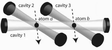
FIG. 1: A possible setup of the three cavities (1, 2 and 3) and the two atomic (aandb) trajectories for the “H configu-ration”.
We will now move on to consider cavity state transfer in a situation where we have three cavities and two atoms. Suppose cavities 1, 2 and 3 are placed so that cavity 1 is overlapping with both cavities 2 and 3. Atomais placed in the crossing between cavities 1 and 2, and atomb in the crossing between cavities 2 and 3, as shown in figure 1. The Hamiltonian for this system is given by
H = 12ωa(σaz+ 1) +12ωb(σbz+ 1) + Ω1ˆa†1ˆa1
+ Ω2ˆa†2ˆa2+ Ω3ˆa†3ˆa3+ [(g1aˆa1+g2aˆa2)σa+
+ (g1baˆ1+g3baˆ3)σb++h.c,
(16)
where σa(b)z, σ+a(b) and σ−a(b) refer to atom a(b), and ˆa†i
and ˆai are the creation and annihilation operators for cavityi. We have denoted the coupling strengths between cavityiand atomaasgia, and correspondingly for atom
b. The number of excitations in the systems is conserved, and we find that the Hamiltonian commutes with the operator
N =1
2(σaz+ 1) + 1
2(σaz+ 1) + ˆa
†
1ˆa1+ ˆa†2ˆa2+ ˆa†3aˆ3. (17) In the following we will assume that Ω1= Ω2= Ω3≡Ω. Otherwise perfect transfer of cavity field states would not be possible, since energy is conserved. In the interaction picture, we form the Hamiltonian
e
H = H−ΩN= ∆a(σaz+ 1) + ∆b(σbz+ 1)
+ (g1aaˆ1+g2aaˆ2)σa++ (g1bˆa1+g3bˆa3)σ+b +h.c.,
(18) where ∆a = (ωa−Ωa)/2, and similarly for b. We now
write the basis states as |n1, n2, n3,±a,±bi, where the
three first entries refer to the number of photons in cavities 1, 2 and 3, and the two last entries to the states of the atoms. The subspaces with exactly one excita-tion in the system is spanned by the five basis states
|0,1,0,−,−i,|0,0,0,+,−i,|1,0,0,−,−i,|0,0,0,−,+i
and |0,0,1,−,−i. Using this ordering of the basis states, the Hamiltonian in matrix form for this subspace becomes
e
H =
0 g2a 0 0 0
g∗
2a ∆a g1a 0 0
0 g∗
1a 0 g1b 0
0 0 g∗
1b ∆b g3b
0 0 0 g∗
3b 0
. (19)
This Hamiltonian has an adiabatic eigenstate with eigen-value zero. Making the Ansatz (C2,0, C1,0, C3)T for this state, the condition on the coefficients Ci becomes
g∗
2aC2+g1aC1=g1∗bC1+g3bCb = 0, so that the adiabatic eigenstate is
|Ψiad=K(g1ag3b,0,−g2∗ag3b,0, g1∗bg2∗a)T, (20)
whereK is a normalisation constant. We see that there should be a possibility of transferring the state of cavity 2 directly to cavity 3 with very little population in cavity 1. For a thorough exposition of adiabatic transfer between atomic levels with multiple intermediate states, see [10]. The theory can be directly applied to cavity state transfer as well. To achieve transfer from cavity 2 to cavity 3, we should start with
|g1ag3b| ≫ |g1bg2a|, (21)
and finish with
|g1bg2a| ≫ |g1ag3b|, (22)
keeping
all the time. There are many possible pulse sequences satisfying these conditions. A few possible coupling se-quences will be discussed in the next subsection. In all cases we start with one field excitation in cavity 2.
As for the case where two cavity modes are coupled by one atom [1], the transfer of arbitrary cavity states from mode 2 to mode 3 will also be possible. If we form the “adiabatic operator”
ˆ
A†(t) =K(t)hg1a(t)g3b(t)ˆa†2−g
∗
2a(t)g3b(t)ˆa†1+g
∗
1b(t)g
∗
2a(t)ˆa
†
3 i
, (24)
where K(t) is a normalisation constant, then, in the adiabatic limit, if we start in the state f[ ˆA†(0)]|0i, we
will also stay in the state f[ ˆA†(t)]|0i as the couplings
are changed. For example, starting in f(ˆa†2)|0,0,−i, we can adiabatically transfer the cavity state to mode 3,
f(ˆa†3)|0,0,−i. As before, this means that we can trans-fer not only one field excitation, but also, for example, number states, where f(A†) =A†n, and coherent states,
wheref(A†) = exp |α|2/2exp(αAˆ†).
B. Numerical simulations of the “H” configuration
For all the numerical simulations in the paper we use Gaussian pulses for the couplings, of the form
giν(t) =Giνexp
−(t−tiν)
2
σ2
iν
. (25)
The index i stands for the i’th cavity and ν for atom
ν; cavities will be labeled with numbers and atoms with letters. If there is only one atom present the atomic index will be omitted. G is the coupling amplitude, and it will be chosen the same for all pulses in the different examples, except for a couple of examples in the next section. The indices will be omitted when theG:s are all the same. The parametertiν gives the pulse center and the width is given byσiν. We are using scaled parameters with ¯h= 1. Timetand the pulse widths σ are given in units of a suitable characteristic timeT, andGand ∆ in units of ¯hT−1.
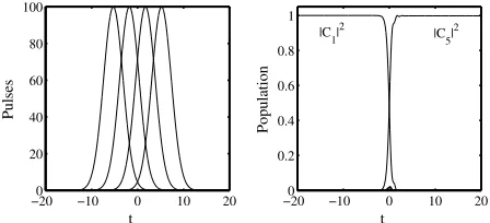
We will consider two possible pulse sequences for adia-batic transfer in the ”H” configuration. The first pulse se-quence, which is shown in figure 2, is completely counter-intuitive, in the sense that we start by coupling cavity 3 and atomb, then cavity 1 and atomb, followed by cav-ity 1 and atoma, and finally cavity 2 and atoma. This could for example be achieved if the cavities are crossing each other horizontally, partly overlapping, and we let the atomb traverse first cavity 3 and then cavity 1, and similarly for atomaand cavities 1 and 2. The parameters in the figure aret3b=−5.22,t1b=−1.72,t1a= 1.78 and t2a = 5.28,σ= 3, ∆ = 0 andG= 100. The dynamics is,
for ∆ = 0, determined by the dimensionless adiabaticity parameterGσ [1].
The pulses are seen in the left plot and the popula-tions in the right one. As shown in figure 2, numerical
−200 −10 0 10 20
20 40 60 80 100
t
Pulses
−200 −10 0 10 20
0.2 0.4 0.6 0.8 1
t
Population
|C
1| 2
|C
[image:4.612.328.552.54.156.2]5| 2
FIG. 2: The figure to the left shows our first example of a pulse sequence for realizing complete population transfer from cavity 2 to cavity 3 with minimal population in the in-termediate cavity 1 for the ”H” configuration. The pulses are ordered in a completely counterintuitive way, from left to rightg3b,g1b,g1aandg2a. Time is given in units of a suitable characteristic timeT. The widths of the pulses are allσ= 3, also in units ofT, and the maximum amplitudes areG= 100 in units ofT−1
. The other plot shows the populations |Ci| 2
(i= 1,2,3,4 or 5) as a function of the scaled interaction time t. It is clear that population is transfered adiabatically from the second cavity (solid line marked|C1|
2
) to the third cavity (dotted line marked|C5|
2
), without remarkable population in cavity 1. The final population in the third cavity is 99.8 %, and maximum population of cavity 1 during the process is 0.2 %.
simulations confirm that an excitation in cavity 2 can be transferred adiabatically to cavity 3, while the pop-ulation in cavity 1 remains small in between. The final population in state|0,0,1,−,−iis 99.8 % and maximum population in cavity 1 is 0.2 % and is located around
t= 0. The coupling amplitudes are rather large in this example in order to have an adiabatic process and corre-spondingly a successful transfer. This is due to the fact that the population virtually passes through three lev-els,|1,0,0,−,−i,|0,0,0,+,−iand|0,0,0,−,+i, instead of just one in the standard STIRAP. However, it is still clear that if the procedure is slow enough it is possible to transfer the population adiabatically. It is also possible to switch the order of the two middle pulses [10].
In this example, the population transfer takes place mainly when all four pulses differ from zero, when the productgprod=g1ag2ag1bg3b6= 0. Lettinggprodincrease
by making the pulses overlap more in time, it is possi-ble to have efficient population transfer from state one to state five with a smaller adiabaticity parameterGσ. However, the price one has to pay is that in this case, the intermediate states become more populated during the evolution, since condition (23) is not as well satis-fied. Thus, there is a tradeoff between strict adiabaticity constraints (largeGσ) and small population of interme-diate states, or weaker constraints but population of the intermediate states during the transfer.
−200 −10 0 10 20 20
40 60 80 100
t (a.u.)
Pulses
−200 −10 0 10 20
0.2 0.4 0.6 0.8 1
t (a.u.)
Population
|C
1| 2
|C
[image:5.612.328.552.52.155.2]5| 2
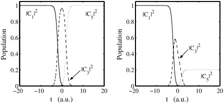
FIG. 3: The same model as in figure 2, but with the second choice of pulse sequence, where the pulses are allowed to have different widths. The pulses, shown to the left, come in the following order: first g1a (solid) and g3b (dotted) at t1a = t3b=−3 and theng1b(solid) andg2a(dotted) att1b=t2a= 3. The widths forg1a and g1b (solid curves) areσ = 6 and for the other two pulses (dotted)σ = 2, and the maximum amplitudes are as in the previous exampleG = 100. Time is given in units of T and the pulse height in units of T−1
. The population transfer, shown in the right plot, is similar to the previous example, with a final population in cavity 3 |C5|
2
= 99.8% and a maximum population in the middle cavity equal to 0.8 %.
the same time. Similarly, the coupling time between atom b and cavity 1 is longer than the coupling time between atom a and cavity 2, and these couplings are also centered around the same time. This coupling se-quence also satisfies the conditions (21 – 23). It could be achieved by making the diameters of laser beams 2 and 3 smaller than the diameter of laser beam 1. Numerical simulations confirm that this coupling sequence works, and the population is transferred from cavity 2 to cavity 3 with very little population of cavity 1 during the trans-fer. The parameters in this second choice for the pulses are,t1a =t3b=−3 andt1b =t2a= 3,σ1a=σ1b = 6 and σ2a =σ3b= 3 and againG= 100. The plot to the right,
for the population transfer, looks similar to populations in figure 2 and here we have final transfer in cavity 3
|C5|2= 99.8 % and maximum population in the middle cavity 1|C3|2 = 0.8 %, thus a small fraction more than in the previous example.
Since cavity 1 remains almost unpopulated for the cou-pling sequences we have discussed, relatively large losses in cavity 1 should not affect the efficiency of the state transfer. This is also confirmed by numerical simula-tions. In order to investigate the effect of losses in the intermediate cavity we add a loss term
δ=e−iγt2 (26)
to the derivative of the amplitude of the state
|1,0,0,−,−i. To check the advantage of our model, with-out population in cavity 1, compared to a situation with population in cavity 1, we simulate a situation were atom
a transfers the photon first to cavity 1 from cavity 2 and then atomb takes it to cavity 3. This amounts to two consecutive ordinary STIRAPs with population in the middle cavity. First we show the population
trans-−200 −10 0 10 20
0.2 0.4 0.6 0.8 1
t (a.u.)
Population
−200 −10 0 10 20
0.2 0.4 0.6 0.8 1
t (a.u.)
Population
|C
5| 2
|C1|2
|C
3| 2
|C1|2
|C5|2
[image:5.612.67.290.54.157.2]|C3|2
FIG. 4: This figure shows the effect of losses in the interme-diate cavity 1. The setup is as a double STIRAP, the first atom transfers the photon from cavity 2 to cavity 1 and fi-nally the second atom brings it into cavity 3. Note that the pulses of the two STIRAP overlap, thus the middle cavity is never fully populated. The pulse parameters are G = 100 (in units ofT−1
), t1a =−3, t2a =−1,t3b = 1 andt1b = 3 and σ1a = σ2a = σ1b = σ3b = 2 (in units of T). The left plot shows the populations without losses in cavity 1, while in the right figure, cavity 1 has a decay rateγ = 0.1. The final population transfer from cavity 2 to 3 is reduced from 100 % to 20 %. This should be compared to, for example, using the pulse sequence of figure 2, with losses. If we add the same decay rateγ= 0.1 for cavity 1 in that process, the population transfer goes down from 99.8 to 99.7 %.
fer without losses in cavity 1 in the left plot of figure 4 and then we add the loss term (26) to the Hamiltonian with a decay rate γ = 0.1 and we see the result in the plot to the right, the transfer efficiency goes down from 100 % to 20 %! When adding the same loss term to the example in figure 2, the decrease in population transfer is only 0.1 percentage units. The parameters for figure 4 aret1a =−3,t2a =−1,t3b = 1, andt1b= 3,σ= 2 and G= 100. If we increase the decay rate toγ = 1, keep-ing all other parameters the same, the population goes down to 99.0 % in our first method, while in the second model, when cavity 1 is populated, no population ends up in cavity 3.
Losses will, however, broaden the lineshape of the cav-ity. If the cavity is too long, factors exp(ikr) coming from the propagation in the cavity will most probably disturb the adiabatic transfer process, since the line is broadened and therefore not only one value, but values of k in an interval are involved. For a long lossy cavity 1, the ef-ficiency of adiabatic transfer from cavity 2 to cavity 3, trying to avoid the lossy cavity 1, will be lowered.
C. Preparation of an EPR state in the ”H” configuration
with eigenvalue zero, and by choosing the pulsesgiν care-fully we could transfer population, but, of course, there are numerous other interesting pulse sequences. Assume that g2a and g3b are turned on simultaneously and then g1a andg1b are turned on simultaneously. The adiabatic
state then begins, att=−∞, as (0,0,1,0,0)Tand ends as (−1,0,0,0,−1)T/√2. Thus, by letting atoma andb interact simultaneously with cavity 2 and 3 respectively, and then simultaneously interact with cavity 1, the ini-tial photon in cavity one will be transfered into anEP R
state,
|EP Ri±=
1
√
2(|0,1i ± |1,0i), (27)
of cavities 2 and 3. This procedure is shown in figure 5. The pulses are given in the left plot and the populations in the right plot. The parameters are t2a = t3b = −2
and t1a = t1b = 2, σ = 3 and G = 5. Note that here
the coupling amplitudes (and correspondingly the degree of adiabaticity) does not need to be as large as in the examples of adiabatic transfer. The photon clearly ends up in cavity 2 and 3. That the state is really the pure state (27), and not a mixture, is checked by calculating the fidelity between the final state from the numerical simulation and theEP R state
F=|+hEP R|ψ(t= +∞)i|. (28)
With the state obtained numerically with the parameters in figure 5, the fidelity becomesF = 0.9999. By control-ling the phases of the coupcontrol-lings it would be possible to obtain differentEP Rstates. Starting with a general field state in cavity 1, the final state would be a more com-plicated entangled state of cavity 2 and 3, obtained with the method explained in the previous section, by acting with the adiabatic operatorf( ˆA†) on the vacuum. The
situation is analogous to when a coherent state is split by a 50/50 beam splitter.
D. ”Star” configuration
We can easily extend the situation to more than three cavities, or to other setups, such as a ring configuration, where the three cavities form a triangle, overlapping each others at the corners of the triangle. In this section we investigate a situation with M cavities and one single atom coupled to all of the cavities, as shown in figure 6. We will also discuss the effect of adding further atoms coupled to some, but not all, of the cavities. If the atom travels along, say, the z-axis, the cavities form a ”star” in thexy-plane. We assume that M −1 of them are in the same plane, centered around z = 0, and cavity M
is slightly shifted fromz = 0. Initially only cavityM is populated and again we take all Ωi’s to be identical.
The effective Hamiltonian for the system is, in the
ro-−200 −10 0 10 20
1 2 3 4 5
t (a.u.)
Pulses
−200 −10 0 10 20
0.2 0.4 0.6 0.8 1
t (a.u.)
Population
|C
3| 2
|C5|2
|C
[image:6.612.327.553.53.162.2]1| 2
FIG. 5: In this figure it is shown how well the method works for preparation of EPR states between cavity 2 and 3. To the left we show the pulses, with the parametersG= 5 (in units ofT−1
),t1a= 2, t2a =−2,t3b =−2 andt1b= 2andσ1a= σ2a=σ1b=σ3b= 3 (in units ofT). The right plot gives the populations, and it is clear that population initially in cavity 1 (solid line) is transfered equally to cavity 2 and 3 (dotted and dashed line). Note that in this situation the amplitude Gis much smaller than in figures 2 and 3. For the fidelity in this example we haveF =|hEP R|ψ(t= +∞)i|= 0.9999.
FIG. 6: This figure shows a possible setup for the ’star’ con-figuration with three cavities. Note that two of the cavities should be in the same plane, while one (the initially populated cavity) is slightly off the plane. The atom passes through the cavities in the middle point of the ’star’.
tating wave and dipole approximation, given by
H = ∆(σa+ 1) +
"
gMaaMˆ σa++ga
MX−1
i=1 ˆ
aiσ+a +h.c
# .
(29) Note that we have assumed that the couplings are iden-tical for the first M − 1 cavities, gia = ga for i =
1,2, ..., M −1. For simplicity, we again consider only
the case with one excitation, N = 1. By labeling the states as|1,0, ..,0,−i, |0,1, ...,0,−i,...,|0,0, ...,1,−iand
|0,0, ...,0,+i, we find the adiabatic eigenstate
[image:6.612.329.553.301.460.2]−200 −10 0 10 20 1
2 3 4 5
t (a.u.)
Pulses
−100 −5 0 5 10
0.2 0.4 0.6 0.8 1
t (a.u.)
Population
|C
4| 2
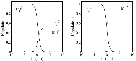
[image:7.612.327.553.52.159.2]|C1,2,3|2
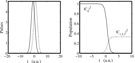
FIG. 7: This shows the numerical simulation of the ’star’ configuration and the preparation of a W state. The left plot gives the pulses in time. The parameters are G = 5, σ1 = σ2 = σ3 = σ4 = 2 and t1 = t2 = t3 = −1 (dotted
lines), t4 = 1 (solid line). Time and the pulse widthsσ are
given in units ofT and the pulse heights are given in units of T−1
. To the right we see the population, and it is easily seen that the initial population in cavity 4 (solid line) is equally transfered to cavities 1, 2 and 3 (dotted lines). The fidelity is F =|hW|ψ(t= +∞)i|= 99.8%.
with eigenvalue zero. Thus, if we have
limt→−∞
gM a
ga
= 0, and limt→+∞
ga
gM a
= 0,
(31) the photon will be adiabatically transfered from cavityM
into all other cavities with equal probability and phase. WithM = 3, the final state in the first two cavities will be anEP Rstate, and withM = 4, we get a so calledW
state,
|Wi=√1
3(|1,0,0i+|0,1,0i+|0,0,1i). (32)
For M > 4, it is possible to prepare the natural
gener-alization of theW state to higher dimensions. A similar setup and the generation of W states were discussed in [17].
In figure 7 we show the pulses and populations during the passage of the atom, with four cavities (M = 4). The parameters are ∆ = 0, G = 5, t1,2,3 = 1, t4 =
−1 and σ1,2,3,4 = 2. The dotted lines shows the pulses
ga(t) and the solid line the pulseg4a(t). The process is
counterintuitive like the original STIRAP. In fact, this is an “ordinary” STIRAP, but withN−1 final states, rather than just a single one. We clearly see that the population is equally split between the first three cavities, and with these parameters the fidelity isF =|hW|ψ(t= +∞)i|= 99.8. Note that, as for the generation of theEP Rstate in figure 5, the amplitudeGis rather small in this example, compared to the case of population transfer between the cavities in the ”H” configuration which is shown in figures 2 and 3.
Next we show how well the process works for differ-ent parameters, changing the coupling amplitudeGand the detuning ∆ between the atomic transition frequency
ωa and the common field frequency Ω. In figure 8, the parameter dependence of the fidelity F = |hW|ψ(t =
0 5 10 15 20
0.92 0.94 0.96 0.98 1
∆ (a.u.)
Fidelity
0 1 2 3 4 5
0 0.2 0.4 0.6 0.8 1
G (a.u.)
[image:7.612.66.290.55.160.2]Fidelity ∆=0 G=5
FIG. 8: This figure shows the fidelityF =|hW|ψ(t= +∞)i| as a function of the coupling-amplitudeG(left plot) and as a function of the detuning ∆ (right plot), for the example given in figure 7. In the first plot ∆ = 0 and in the secondG= 5 (in units ofT−1), otherwise the parameters are as in the previous figure 7.
+∞)i|, in the previous example, is shown; first as func-tion of the amplitudeG, with ∆ = 0, and then as function of ∆, withG= 5. The other parameters are as in figure 7. The fidelity, as expected, increases with the coupling and decreases with the detuning. Similar plots could be made for the other examples, and the information ob-tained would be similar.
In section II we explained how a general Fock state
|niis adiabatically transfered between two cavities. The same procedure can, of course, be used also in this con-figuration. In a similar fashion as in equation (9), we introduce an ”adiabatic operator”. Using the pulse se-quence above, the adiabatic state (30) will then evolve according to
|0, ...,0, n,−i → X
k1 +...+kM−1=n
1
N n!
k1 !...kM−1!
ˆ
a†1
k1...ˆa†
M−1 kM−1
|0,−i,
(33)
where|0,−ion the right hand side means vacuum plus ground state atom and 1/N is a normalization constant. Here we have also used the multinomial theorem. Know-ing how a Fock state transforms, it is easy to calculate how a general state in cavityM evolves. States of sim-ilar forms as the one above, but for two modes, have been discussed for example in [18, 19]. By selecting the coefficients in equation (29) to differ between the indi-vidual modes, more general final states can be prepared adiabatically.
In the adiabatic limit the system evolves according to the adiabatic states, and the process is robust against small changes in the parameters [20], which is a great ad-vantage for example in quantum computing [21, 22]. The adiabatic states are, however, sensitive to small changes in the Hamiltonian, which will be shown next. If a second atomb, also in its ground state, is coupled to only cavity
jin the ”star” configuration during the whole passage of the first atom through theM cavities, we have to add an interaction term to the Hamiltonian (29) of the form
V =gjbˆajσb++h.c. (34)
and the second atomb is zero, so in the interaction pic-ture the atomic energy vanishes. The shape ofgjbis not so important as long as it is non-zero during the pro-cess. We take it to be constant, but it could also be a very broad Gaussian, so that it extends outside the other Gaussian pulses ga and gMa, which could be the situa-tion if the second atom moves much slower than the first atom and only through the j’th cavity. By adding the term (34) to the original Hamiltonian, the Hilbert space dimension obviously increases by one unit, due to the state |0,0, ..,0,−,+i, and the corresponding adiabatic state (30) becomes
|Ψiad=K(−gMa,−gMa, . . . ,0, . . . ,−gMa, ga,0,0)T,
(35) where the new 0 is on thej’th position. The added atom thus takes away the population in thej’th cavity. In the adiabatic limit, the magnitude of gjb is not important, just that it is non-zero. In other words, coupling one of the ’bare’ states in the Hamiltonian weakly to a ’new’ state drastically affects the adiabatic evolution. If a new atomcor atombis coupled to yet another cavitylduring the whole interaction, the population of that state would become zero.
The modification in the evolution is shown in figure 9. We use exactly the same example and parameters as figure 7, except that the common amplitude is nowG= 50. In the left plot a second atomb has been coupled to the third cavity with a constant couplingg3b=G3b= 5,
and it is seen that all of the photon ends up in cavity 1 and 2. Note that atomais coupled ten times as strongly to the field as atomb. In the plot to the right, a further third atomc is coupled with a constant couplingg2c = G2c= 5 to cavity 2, and all population now ends up in the
first state, namely the photon is in cavity 1. These plots clearly show how a small disturbance to the adiabatic Hamiltonian changes the evolution. IfGwould have been made larger, the perturbations could have been made smaller.
IV. STATE PREPARATION USING ADIABATIC TRANSFER AND ATOMIC MEASUREMENTS
In the previous sections the atom remained more or less in its lower state during the whole process and could be seen as an ancillary state, which is never very en-tangled with the field state. Assuming perfect detec-tion efficiency, a measurement on the atomic state in the
|±i-basis, after the interaction, would give|−iwith unit probability. As long as the atomic state does not get entangled with the field states, an atomic measurement would not modify the cavity states.
By introducing a third atomic level|qi, which does not interact with the field, it is possible to create atom-field entanglement. Thus, an atom in the state |qi will pass through the cavities without any interaction, which could be due to a large detuning or selection rules. The Hamil-tonian is correspondingly only modified by the term for
−100 −5 0 5 10
0.2 0.4 0.6 0.8 1
t (a.u)
Population
−100 −5 0 5 10
0.2 0.4 0.6 0.8 1
t (a.u)
Population
|C4|2
|C2|2
|C1|2
[image:8.612.327.554.51.154.2]|C4|2 |C1|2
FIG. 9: This figure shows the dynamics of the same ’star’ configuration as in figure 7, but with small perturbations to the Hamiltonian. The left plot shows the same evolution as in figure 7, but now with a second atombcoupled, in its ground state, to the cavity 3. The coupling amplitudeG between the first atoma and the four cavities are now G= 50, but all other parameters are the same as the previous example. The coupling between atomband cavity 3 is constant during the process,g3b=G3b= 5, and the corresponding detuning is zero. The added atom-cavity interaction clearly modifies the evolution so that the photon ends up in cavity 1 and 2 (dashed and dotted lines). To the right we have added yet a third atomc, also with a constant couplingg2c=G2c= 5 and zero detuning, interacting with cavity 2, and now the population in that state is removed, so that only cavity 1 is populated (dotted line). Note that atom b and c is much weaker coupled to the fields than atoma. Time is given in units ofT and pulse heights in units ofT−1
.
the atomic energy in state|qi, which could, of course, be omitted in a rotating frame.
In this section we will look at the ”H” configuration, but other setups could also be considered. We will show how it is possible to create entangled Schr¨odinger cat states [23, 24, 25] by measuring the atomic state after the interaction. We introduce the atomic states
|χia,b± =
1
√
2 |−i
a,b
± |qia,b, (36)
where the indices a and b refer to the different atoms. We will first couple cavities 1 and 2. From the STIRAP evolution
|0, α,−i −→ | −α,0,−i
|0, α, qi −→ |0, α, qi
(37)
for coherent states, it follows, starting from one of the atomic states (36) in the ”H” configuration, that
|0, α,0i|χia+ −→ 1
√
2(| −α,0,0i|−i
a+
|0, α,0i|qia).
(38) After the interaction, the atom is measured in the|χia
±
-basis, and depending on the measurement result the field will be in the state
N| −α,0,0i+ (−1)i|0, α,0i, (39)
wherei= 0 for the measurement outcome|χia
+andi= 1 for the result |χia
−, and the normalisation constant is
The atomic measurement in the desired basis can be effected by first using Raman pulses to couple the atomic states|−iand|qi. The resulting unitary evolution should transform |χi+ into |−i and |χi− into |qi, so that the
measurement can then be implemented by testing for population in the levels |−iand |qi with a fluorescence measurement. With this procedure it is possible to reach a very high measurement efficiency, almost 100%. Sim-ilar methods can be used to implement also generalised quantum measurements on atoms or ions [26].
A second atom is then injected into cavity 1 and 3 in the state|χib
+. The state will evolve into
N √
2
|0,0, αi|−ib+| −α,0,0i|qib
+(−1)i|0, α,0i|−ib+ (−1)i|0, α,0i|qib.
(40)
Atom b is then measured in the same basis as that for atoma, with the result proportional to
|0,0, αi+(−1)j|−α,0,0i+(−1)i|0, α,0i+(−1)i+j|0, α,0i,
(41) for the cavity field states, wherej is defined asi is, but for atom b. We have here left out the normalising con-stant, since it will depend on the measurement outcome for atomb. Depending on the known measurement out-comes for atoms a and b, we are able to prepare four possible entangled states,
|Ψ00i ∝(| −α,0,0i+ 2|0, α,0i+|0,0, αi), i=j= 0
|Ψ01i ∝(−| −α,0,0i+|0,0, αi), i= 0, j= 1
|Ψ10i ∝(| −α,0,0i −2|0, α,0i+|0,0, αi), i= 1, j= 0
|Ψ11i ∝(−| −α,0,0i+|0,0, αi), i=j= 1.
(42) We may also consider the following scenario. If the second atom is injected in the state|−ib instead, it will
leave the setup in the same state, and the resulting field state is
N |0,0, αi+ (−1)i|0, α,0i. (43)
Let us fixβ throughα= 2β and introduce the displace-ment operatorD with the properties
D(β)|αi=eiIm(αβ∗)|α+βi. (44)
If the operator D(−β) is applied to both cavity 2 and 3 and for realα and β, the resulting entangled state of cavities 2 and 3 becomes
N | −β, βi+ (−1)i|β,−βi, (45)
where N is defined as before. Here cavities 2 and 3 are both in a Schr¨odinger cat state and entangled with each other. This kind of entangled state is of great interest for quantum teleportation [27] and quantum computing with
coherent states [28], but also for studying quantum phe-nomena in general, like entanglement and decoherence in the classical limit [29]. Using a 50/50 beam splitter, this state may be transformed into|√2β,0i+(−1)i|−√2β,0i,
i.e. a cat state in one of the modes only, with vacuum in the other mode.
It should be mentioned that the atomic states |χi±
could have been defined in different ways, leading to other entangled field states. The initially prepared and mea-sured atomic basis need not be the same. We could have considered different setups of cavities and atoms and the initial coherent state could have been any state, for ex-ample squeezed states.
We conclude this section by considering another exam-ple of how to prepare a Schr¨odinger cat state. We now assume just two overlapping cavities and a single atom as in section II. The difference is that the atoma now should have (at least) two degenerate ground state levels
|−iI,IIlabeled by I and II, such that the coupling ampli-tudes areG1a,I =G2a,I =G1a,II =Gand G2a,II =−G, where 1 and 2 indicate the cavity and I,II the transition. One way to achieve this might be to impose a chosen quantization axis for the atom using an external electric field, thus forcing the dipole moment dof the atom to
have the suitable components along the directions of the two laser fields. Alternatively it may be possible to use selection rules for the transitions in such a way, that it is possible to choose the signs of the electric field com-ponents inducing the different transitions. The choice should be made in such a way that d·E has the
re-quired signs for the four different combinations of laser and atomic transition.
Assuming that this choice of coupling constants is pos-sible, if we now prepare the atom in state|−iaI, an initial coherent state |α,0i in mode 1 will be transferred into
|0,−αi in mode 2. This is because as we can see from the discussion in section II A, whenG1a,I/G2a,I >0, then an arbitrary field statef(ˆa†1)|0iin cavity 1, will be trans-ferred into a statef(−ˆa†2)|0iin cavity 2. But if the atom is prepared in |−ia
II, an initial coherent state |α,0i in mode 1 will be transferred into|0, αiin mode 2,without the minus sign. Again, this is becauseG1a,II/G2a,II<0, so that an arbitrary field state in cavity 1,f(ˆa†1)|0i, will be transferred into a state f(ˆa†2)|0i in cavity 2. If the atom is initially in a superposition of the two states,
|ψia ±= 1/
√
2(|−ia
I ± |−iaII), the result will be
|α,0i|ψia± −→ √1
2(|0,−αi|−i
a
I ± |0, αi|−iaII). (46) This is a Schr¨odinger cat state for cavity 2 and the atom. If we wish to disentangle the atom and the cavity, the atom may be measured in the basis 1/√2(|−ia
I ± |−iaII). Depending on the measurement outcome, we are left with one of the states
N(|0, αi ± |0,−αi). (47)
V. CONCLUSIONS
In this paper, we have given several examples of cav-ity field state preparation and transfer using adiabatic methods. The technique we use is related to stimulated Raman adiabatic passage (STIRAP) [2, 3]. In standard STIRAP, atomic energy levels are coupled by laser pulses in order to transfer population between the atomic states. In the present scheme, cavity field mode are effectively coupled by atoms in order to transfer population between the cavity modes. A previous paper showed that not only photon number states, but arbitrary cavity field states can be transferred using this method [1]. In this paper, we have in particular considered preparation of entan-gled states of two or more cavities, such as anEP Rstate and a W state, and various entangled superpositions of coherent states in different cavities. The theoretical con-siderations are supported by numerical simulations. It may also be possible to use similar techniques in solid state systems, replacing the cavities and atoms in our discussion with cavities coupled to Josephson junctions [30].
One advantage of adiabatic state transfer and prepa-ration methods is that they are relatively robust against changes in the individual coupling pulse strengths and pulse durations. In contrast, state transfer e.g. in the Jaynes-Cummings model [15] relies on the ability to ex-perimentally control the areas of coupling pulses very ac-curately. The situations considered in this paper are by no means totally unrealistic considering the present sta-tus of experiments in QED. An important condition is that all the cavity modes have to be degenerate. This results from energy conservation; if the modes were not degenerate, perfect state transfer between modes would not be possible. The adiabaticity for processes like the ones considered in this paper, is roughly given by the
coupling amplitude times the pulse widthGσ, see [1]. In the example of figure 2 we have Gσ = 300, while us-ing typical experimental values ofG/2π∼100 MHz and
σ∼0.3 s−1 [8, 31], the adiabaticity parameter becomes
Gσ≈200. With these characteristic non-scaled parame-ters, the coupling is multiplied by 2π·106 and the time scales by 10−7, the adiabatic transfer of figure 2 gives a final population of 96.9 % in the target cavity, while the maximum population in the intermediate cavity 1, during the process, is 2.2 %. The whole operation, with the two atoms passing through the three cavities, takes about 2µs, which is much shorter than the characteristic life times of cavity and the atomic states [31]. Remem-ber, that the example of adiabatic transfer in figures 2 and 3 involves more virtual intermediate levels than, for example in the generation ofEP Rand W states in fig-ures 5 and 7. Another point to emphasize is that, as the field amplitude increases, the number of intermedi-ate stintermedi-ates also increases, which makes the adiabaticity constrains stricter. Even though it is possible to have strong enough couplings and small decay rates for realiz-ing the schemes proposed in this paper, it is not obvious whether it is a simple task to add crossing cavities in current experimental setups.
In conclusion, adiabatic techniques offer rich possibili-ties for state transfer and population.
Acknowledgments
We would like to thank Prof. Stig Stenholm for in-spiring discussions and comments. E. A. acknowledges financial support from the Royal Society in the form of a Dorothy Hodgkin Fellowship and useful comments from Prof. Erling Riis.
[1] F. Mattinson, M. Kira and S. Stenholm, J. Mod. Opt.
48, 889 (2001).
[2] F. T. Hioe, Phys. Lett. A99, 150 (1983).
[3] K. Bergmann, H. Theuer, and B. W. Shore, Rev. Mod. Phys.70, 1003 (1998).
[4] F. Mattinson, M. Kira and S. Stenholm, J. Mod. Opt.
49, 1649 (2002).
[5] M. Amniat-Talab, S. Gu´erin, N. Sangouard and H. R. Jauslin, e-print quant-ph/0407233 (2004).
[6] A. Biswas and G. S. Agarwal, J. Mod. Opt., 51, 1627 (1991).
[7] A. S. Parkins, P. Marte, P. Zoller, O. Carnal and H. J. Kimble, Phys. Rev. A51, 1578 (1995).
[8] W. Lange and H. J. Kimble, Phys. Rev. A, 61, 063817 (2000).
[9] J. Larson and S. Stenholm , J. Mod. Opt. 50, 1663 (2003).
[10] N. V. Vitanov, Phys. Rev. A58, 2295 (1998).
[11] Y. B. Band and P. S. Julienne, J. Chem. Phys.95, 5681 (1991).
[12] N. V. Vitanov and S. Stenholm, Phys. Rev. A60, 3820 (1999).
[13] B. W. Shore, K. Bergmann, J. Oreg and S. Rosenwaks, Phys. Rev. A44, 7442 (1991).
[14] V. S. Malinovsky and D. J. Tannor, Phys. Rev. A56, 4929 (1997).
[15] B. W. Shore and P. L. Knight, J. Mod. Opt. 40, 1195 (1993).
[16] T. A. Laine and S. Stenholm, Phys. Rev. A 53, 2501 (1996).
[17] M. Yang, Y. M. Yi and Z. L. Cao, Int. J. Quant. Inform.
2, 231 (2004).
[18] C. Wildfeuer and D. H. Schiller, Phys. Rev. A67, 053801 (2003).
[19] B. Deb, G. Gangopadhyay and D. S. Ray, Phys. Rev. A
48, 1400 (1993).
[20] A. M. Childs, E. Farhi, and J. Preskill, Phys. Rev. A65, 012322 (2001).
[22] M. S. Shahriar, J. A. Bowers, B. Demsky, P. S. Bhatia, S. Lloyd, P. R. Hemmer and A. E. Craig, Opt. Commun.
195, 411 (2001).
[23] J. Larson and B. M. Garraway, J. Mod. Opt.51, 1691 (2004).
[24] E. Solano, G. S. Agarwal and H. Walther, Phys. Rev. Lett.90, 027903 (2003).
[25] G. S. Agarwal and R. R. Puri, Phys. Rev. A 40, 5179 (1989).
[26] S. Franke-Arnold, E. Andersson, S. M. Barnett, and S. Stenholm, Phys. Rev. A63, 052301 (2001).
[27] T. J. Johnson, S. D. Bartlett and B. C. Sanders, Phys. Rev. A66, 042326 (2002).
[28] H. Jeong and M. S. Kim, Phys. Rev. A65, 042305 (2002). [29] D. F. Walls and G. J. Milburn, Phys. Rev. A31, 2403 (1985); S. J. D. Phoenix, Phys. Rev. A41, 5132 (1990). [30] Z. Kis and E. Paspalakis, Pys. Rev. B69, 024510 (2004); A. D. Greentree, J. H. Cole, A. R. Hamilton, and L. C. L. Hollenberg, e-print cond-mat/0407008 (2004). [31] C. J. Hood, T. W. Lynn, A. C. Doherty, A. S. Parkins