Rochester Institute of Technology
RIT Scholar Works
Theses
Thesis/Dissertation Collections
6-1-2002
Support vector machines for image and electronic
mail classification
Matthew Woitaszek
Follow this and additional works at:
http://scholarworks.rit.edu/theses
This Thesis is brought to you for free and open access by the Thesis/Dissertation Collections at RIT Scholar Works. It has been accepted for inclusion
in Theses by an authorized administrator of RIT Scholar Works. For more information, please contact
Recommended Citation
Support Vector Machines for
Image and Electronic Mail Classification
by
Matthew Stephen Woitaszek
A Thesis Submitted
III
Partial Fulfillment of the
Requirements for the Degree of
Masters of Science
III
Computer Engineering
Dr. Muhammad Shaaban
Assistant Professor, Department of Computer Engineering
Dr. Andreas Savakis
Associate Professor, Department of Computer Engineering
Dr. Roy Czemikowski
Professor, Department of Computer Engineering
Department of Computer Engineering
Kate Gleason College of Engineering
Rochester Institute of Technology
Rochester, New York
Release Pennission Fonn
Rochester Institute of Technology
Support Vector Machines for
Image and Electronic Mail Classification
I, Matthew Woitaszek, hereby grant permission to the Wallace Library of the Rochester
Institute of Technology to reproduce my thesis in whole or in part, on or after July 1,
2002. Any reproduction will not be for commercial use or profit.
ABSTRACT
Support Vector Machines
(SVMs)
have demonstrated
accuracy
andefficiency
in
avariety
ofbinary
classification applicationsincluding
indoor/outdoor
scene categorizationof consumer photographs and
distinguishing
unsolicited commercial electronic mailfrom
legitimate
personal communications.This
thesis
examines a parallelimplementation
ofthe
Sequential Minimal Optimization
(SMO)
method oftraining
SVMs
resulting in
multiprocessor
speedup
subjectto
adecrease
in
accuracy
dependent
onthe
data
distribution
and number of processors.Subsequently
the
SVM
classification system wasapplied
to
the
image
labeling
and e-mail classification problems.A
parallelimplementation
ofthe
image
classification system's colorhistogram,
colorcoherence,
and edge
histogram feature
extractorsincreased
performance whenusing both
non-caching
andcaching
data
distribution
methods.The
electronic mail classificationapplication produced an
accuracy
of96.69%
with a user-generateddictionary.
An
implementation
ofthe
electronic mail classifier as aMicrosoft Outlook
add-in providesimmediate
mailfiltering
capabilitiesto the
averagedesktop
user.While
the
parallelimplementation
ofthe
SVM
trainer
was not supportedfor
the
classificationapplications,
TABLE OF CONTENTS
Table
ofAppendices
ii
List
ofFigures
iii
Acknowledgements
iv
Glossary
vIntroduction
andBackground
1
1.1
Feature-Based SVM Classification Systems
2
1.2
Other Classification Techniques
3
1.3
Support
Vector Machines
5
1.4
Image
Classification
7
1.5
Electronic
Classification
8
Support Vector
Machine
Theory
andOperation
11
2.1
Support
Vector
Machines
1 1
2.2
Sequential
Minimal Optimization
15
Parallelization
ofSequential
Minimal Optimization
20
3.1
Interleaved Parallelization
25
3.2
Blocked Independent Parallelization
27
3.3
Results
29
3.4
Discussion
31
Parallel Image
Classification
34
4.1
Color Feature Extraction
36
4.2
Texture Feature Extraction
38
4.3
Combined
Feature Extraction
andClassification System
40
4.4
Accuracy
Results
44
4.5
Performance
Results
46
4.6
Discussion
47
Electronic Mail Classification
55
5.1
Data
Sets
56
5.2
Method
57
5.3
Results
58
5.4
Discussion
59
5.5
Microsoft
Outlook
Integrated
Spam
Scanner
62
Conclusions
64
6.1
Summary
ofWork
64
6.2
Challenges Encountered
65
6.3
Future Work
66
TABLE
OF APPENDICES
Appendix
A
-SVM Software Operation
71
Appendix B
-Parallel
SVM Results
73
Appendix
C-Full
Image Individual
Classifier Results
74
Appendix D
-Full
Image
Combined Classifier Results
77
Appendix E
-Subblocked Image
Individual
Classifier
Results
79
Appendix
F
-Subblocked
Image
Combined Classifier Results
80
Appendix
G-Image
Feature Extraction
Performance
81
Appendix H
-Image Classification Output
Example
82
Appendix I
-MailClassification Test
Sets
84
Appendix J
-Classification Results
85
Appendix
K
Classification Trained
Dictionary
Model
86
Appendix L
-Classification Interface
89
Appendix M
Classification
Outlook Integration
90
Appendix N
LIST OF FIGURES
Figures
Figure 1.1
-SVM data flow block diagram
2
Figure 2.1
-Separating
hyperplanes in
alinear SVM
12
Figure
2.2
-Constraints for optimizing
two
Lagrange
multipliers17
Figure
3.1-Optimization
patternfor
two
way
parallelinterleaved
approach26
Figure 3.2
-Optimization
partemfor
three
way
parallelinterleaved
approach26
Figure
3.3
-SVM
recall
for Adult
Linear
30
Figure
3.4-SVM
performancefor
Adult Linear
30
Figure
3.5
-SVM
recall
for Adult
RBF
30
Figure
3.6
-SVMperformancefor
Adult RBF
30
Figure
4.1
-Pixel
enumeration
for
3x3
gridSobel
operator39
Figure
4.2
-Two
stage classification approach41
Figure 4.3
-Execution
trace
before
parallelization42
Figure 4.4
-Execution
trace
after parallelization52
Tables
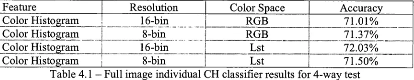
Table 4.1
-Fullimage individual CH
classifier resultsfor
4-way
test
37
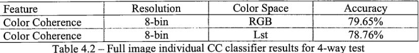
Table 4.2
-Full
image individual CC
classifier resultsfor
4-way
test
38
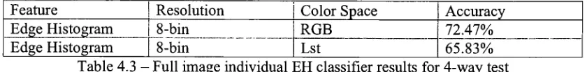
Table
4.3
-Fullimage individual
EH
classifier resultsfor
4-way
test
40
Table
4.4
-Parallel
feature
extractor processor assignments42
Table 4.5
-Finalfull image
individual
classifieraccuracy
45
Table 4.6
-Final
full image
combined classifieraccuracy
45
Table 4.7
-Finalsubblockedimage individual
classifieraccuracy
45
Table
4.8
-Final
subblockedimage
combined classifieraccuracy
45
Table 4.9
-Feature
extractionperformance46
Table 4.10
-Imageclassificationperformance47
Table 4.11
-NumberofSVs in feature
classifier models53
Table 5.1
-MailClassification
Accuracy
59
Table 5.2
-Trained
ACKNOWLEDGEMENTS
Research
withoutindebtedness is
suspect,
andsomebody
mustalways,
somehow,
be
thanked.
-UmbertoEco,
How
to
Write
anIntroduction
I
wouldlike
to take
this
opportunity
to
thank
severalindividuals for
their
contributions
to this thesis.
First
andforemost is
my
thesis
advisor, Dr. Muhammad
Shaaban,
whointroduced
meto
parallelcomputing
and wasinfluential
in
the
development
ofthis
project as well asmy
selection offuture
graduate work.Dr.
Roy
Czernikowski
andDr.
Andreas
Savakis
consistently
appliedtheir
high
standards ofacademic
rigor,
ensuring
that
my
work was completed ontime,
underbudget,
anddone
right.
Several
other people providedfantastic
assistancemaking
portions ofthis
workpossible.
I
mustthank
Navid
Serrano
ofKodak
for
substantial supportin
understanding
the
applications of support vector machinesto
image
processing
andSue Muller for
awalkthrough of
her feature
extractionthesis
project.Shawn
Thomas,
ofRIT Information
Technology
Services,
providedthe
unsolicited commercial electronic mailfor
the
spamfilter
training.
Within
the
Department
ofComputer
Engineering,
Rick Tolleson
andPaul
Mezzanini
provided assistance with computational resources.Finally,
I
amespecially
thankful
for
the support, encouragement,
andproofreading
abilities ofmy
mother,
Lynn
GLOSSARY
CC
-Color
Coherence.
A
feature
vectorfor image
classification producedby
generating
a colorhistogram
including
only
points surroundedby
a region of colors within a specifiedtolerance
(p. 37).
CH
-Color Histogram. A feature
vectorfor image
classificationdescribing
the
quantities of constituent colors
in
animage (p.
36).
EH
-Edge Histogram. A
feature
vector
for image
classification producedby
generating
an angle
histogram
afterthe
Sobel
edge-detectiontransform.
The
edgehistogram
produces
texture-related
image data (p.
40).
KKT
-Karush-Kuhn-Tucker
conditions.
Necessary
and sufficient conditionsfor
the
termination
of aSVM
training
process with a valid solution(p. 14).
k-NN
-k-Nearest Neighbor
classifier.A
classification system which calculatesthe
distance between
a sample point and alltraining
samps; the
new pointis
in
the
same
category
asthe
majority
ofits k
nearest neighbors(p. 4).
Osuna's
method.A
methodfor
ttaining
SVMs
by fixing
the
size ofthe
quadraticproblemand
cycling
through the
entire sample space(p.
5).
QP
-Quadratic
Programming
problem.Memory
andtime
intensive
numerical method usedto train
SVMs
using
brute force
andlarge
matrices,
enhancedby
Osuna's
method and
SMO
(p.
14).
RBF
-Radial Basis Function. A
nonlinearkernel
usedfrequently
in
SVM
training.
The
RBF
kernel
mapsnonlinearly
separabledata into
adifferent
space soit
may
be
used
for
classification(p.
71,
see also p.1 1+).
SMO
-Sequential Minimal Optimization. A
method
for
training
SVMs
by
optimizing
two
vectors at atime
analytically instead
ofusing
a numeric quadratic problemsolver,
developed
by
Piatt in 1997
(p.
15).
SV
-Support Vector.
A feature
vectorselected
through
optimizationfor
inclusion in
asupport vector machine model
(p.
12).
SVM
-Support Vector Machine. A
systemfor
performing
automated classificationoffeature
vectorsby locating
ahyperplane
separating
the
target
groupsin
multidimensional
space,
developed
by
Vapnik
andChervonenkis
in
1979
(p.
5).
UCE
-Unsolicited Commercial E-mail. Junk
Chapter
1
Introduction
and
Background
High-level
textual
and pictorial contentrecognition, classification,
andsorting
continue
to
be challenging
andactively
researched areas ofinterest.
Programming
acomputer
to
performbinary
classifications,
such asidentifying
faces in
animage
orflagging
news articles ofinterest
to
a particularperson,
represent a substantialtheoretical
and computational
task.
Support
Vector Machines
(SVMs),
atype
offeature-based
classification
system,
provide an efficient and accurate mechanismfor
this type
ofautomated classification
[12]. SVM
classification systems are capable ofhigh-accuracy
classification while
maintaining
acceptable modeltraining time,
sampletesting
time,
andsystem storage requirements.
The
purpose ofthis thesis
is
to
examinethe
operation ofthe
SVM
sequentialminimal optimization
training
algorithm andits
applicationto
two
classificationproblems.
The
first
sectiondescribes
the
process oftraining
aSVM using
sequentialminimal optimizationand
two
possibleapproachesto
improve
performanceusing
parallelprocessing.
The
secondandthird
sectionsdescribe
the
classification applicationsthat
areof particular
interest for
this
thesis.
The
first
problem,
whichdeals
with scannedconsumer
photographs,
labels
each photograph asdepicting
anindoor
or an outdoorscene.
The
secondproblem,
whichusestextual
features,
labels
electronic mail messages1.1
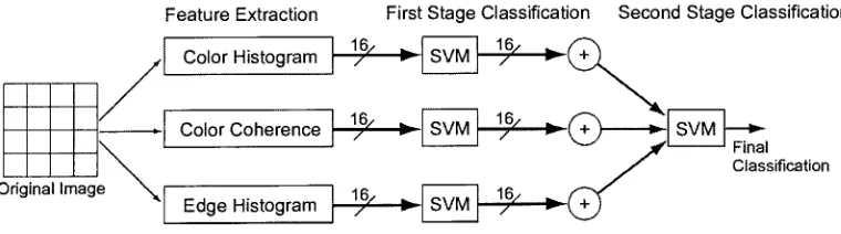
Feature-Based SVM Classification Systems
The
construction of afeature-based
classificationsystem,
such as oneutilizing
SVMs,
occursin
two
phases:training
andtesting
(see Figure
1.1). In
the
training
phase,
aseries of representative samples
from both
positive and negative categories are obtainedand
manually
labeled.
These
samples are utilizedby
the
training
processto
create aclassification model.
Training
is generally
avery
lengthy,
time-consuming
process,
andis
performed
only
once.After
a system modelhas been
obtained,
the
systemmay
be
usedto
perform classifications of new samples
very
quickly.Training
Process
Feature
Vectors
Training
Documents"
Feature
Extraction
Training
Testing (Classification)
Process
Unknown_
Document
Feature
Extraction
Feature Vector
Learned
Model
(Support
Vectors)
Classification
__Labeled
[image:11.506.74.435.281.420.2]Document
Figure 1.1
-SVM data
flow block diagram
SVMs do
notclassify
complex rawdocuments,
such astext
orimages,
directly.
Instead,
the
SVM
training
or classification process starts with afeature
extraction stage.Feature
extraction performs a consistent algorithmic reduction on adocument,
generating
a simpler representative
description
ofthe
sample's pertinent properties.The
series ofproperties extracted
from
a sampleis
referredto
as afeature
vector,
andthe
number oftotal
features
possiblefrom
all samplesis
the
feature
space.When working
withtext
documents,
for
example,
words canbe features.
The
feature
space contains all ofthe
particular word appears
in
adocument
or whether or not a word appeared at all.Feature
vectors generated
by
textual
documents
aregenerally
sparse,
andthe
feature
vectorcontains a small number of
identified features from
avery
large feature
space.Feature
vectors generated
by
examining images
aretypically
dense,
containing data from
scaledmetrics.
For example,
a colorhistogram
may
be
generatedby
afeature
extractorfor
afull
image
orblocked
portions of animage,
creating
afeature
vector withthe
number offeatures
equalto the
number ofbins in
the
histogram. Regardless
ofthe
data type,
the
selection of an appropriate
feature
extraction scheme remains an essential component ofeffective classification system
design.
The
selectedfeature
vectors mustadequately
represent
the
difference between
categoriesfor
classificationto
be
possible.1.2
Other
Classification
Techniques
SVMs
areonly
one of severaltechniques
availableto
perform automatedclassification
based
onfeature
vectors.Other
techniques,
such asinductive
rule-basedclassifiers,
neuralnetworks,
probabilistic and statisticalmodels,
and geometricnearest-neighbor
classifiers,
have
alsodemonstrated
usefulnessin
classifying
adiverse
range ofdata.
The
selection of a classificationtechnique
for
an application requires evaluation ofthe
method'straining
time,
classification executiontime,
storage requirements andsimplifying
assumptions,
as well asthe
ease ofincorporating
newdocuments into
apreviously
trained
system.One
ofthe
oldest approachesto
machine classificationusesinductive
learning
to
instead
offeature
vectors,
these
algorithms produce a series ofif-then
clausesrepresenting
alogical
conjunction whichmay
be
evaluatedvery quickly
to
classify
a newdocument.
Ripper,
for
example,
constructs rulesto
designate
whichdocuments
may
be
labeled in
the
positiveclass,
andthen
includes
assertions whichmay
be
usedto
prunefalse
samples.Rule-based
approacheshave
the
advantage ofbeing
easily
readable andmodifiable
by
humans
and allow usersthe
opportunity
to
specify
prior or posteriorconstraints.
Unfortunately,
the
rule construction processgenerally
requires an extremesimplification of a
document's
feature
space,
and can still require substantialcomputational
time.
Neural
networks and probabilistic classifiers aretwo
other approachesto
automated classification.
Neural
networks canbe
constructedto
learn
nonlinear mappingsbetween features
and categories[17],
although acceptable performanceis
achievedonly
by limiting
the
dimensionality
ofthe
feature
space.Probabilistic
classifiers,
such asthe
naive
Bayes classifier,
assumethat
individual
features
arecompletely
independent,
andagain require
dimension
reduction[9].
Another
classificationmodel, the
k-Nearest Neighbor
(k-NN)
classifier,
uses ageometric approach
to
determining
samplesimilarity
[9].
Each
sampleis
mappedinto
amultidimensional
feature
spaceusing
afunction
whichgroups similar samplesin
clusters.To classify
a newsample, the
distance
from
the
new pointto
every
training
sample pointis
calculated,
andthe
new pointis labeled
the
same asthe
majority
ofits k
nearestneighbors.
The
evaluationtime
ofthe
classifieris
directly
relatedto
the
number ofsamples contained
in
the
system,
and canbecome
prohibitively
large if
a complexSVMs
reducethe
evaluation-time computationalcomplexity
presentin k-NN
classifiers
by determining
the
separationboundary
between
the two
cases.Instead
ofcomparing
a new pointto
every
training
point,
aSVM
simply
determines if
a new pointis
above orbelow
the
separating
boundary
to
produce a classification.Training
aSVM
requires
locating
this
separating
hyperplane,
andforms
the
basis
ofSVM
theory
development.
1.3
Support Vector
Machines
The
statisticallearning
theory
behind SVMs
wasoriginally
developed
by
Vapnik
and
Chervonenkis in
1979,
andits
related concepts of structuralrisk
minimization andsupport vector regression are
frequently
referredto
asVC
theory
[2]
[7]. The
originalmathematical
foundation
ofSVM
training
requiresthe
minimization of afunction
expressed as a
Lagrangian
representedby
amatrix,
sobrute force
training
makesextensive use of a quadratic
programming
(QP)
solverin its innermost loop. Several
approaches
to
facilitate faster
andless
computationally
intensive
SVM
training
have been
developed
[11]
[12].
Training
a singlelarge SVM
withQP
methods uses substantial amounts ofmemory
by
requiring
a matrix capable ofstoring
the
number of samples squared[12].
Vapnik
initially
suggestedtraining
aSVM
with atechnique
known
aschunking,
whichsolves portions of
the
QP
problemto
identify
andremoverowsand columnsevaluating
to
zero, thus
reducing
the
size ofthe
problembefore solving
it
completely.To
increase
of smaller
QP
subproblems.The
algorithm maintains a constant sizeQP
matrixin
the
solver, adding
new untrained samples whileremoving properly
trained
samplesbetween
each step.
Both methods,
however,
still utilizeQP solvers,
whichPiatt
notes arenontrivial and require substantial attention
to
detail: "Numerical QP is notoriously
tricky
to
getright;
there
aremany
numerical precisionissues
that
needto
be
addressed"[12,
p.5]. Most
numericSVM
solvers utilizeprofessionally designed QP
packagesto
performthe
appropriate computationsduring
the
algorithm's execution.To
eliminatethe
complexity
andinefficiency
ofusing
aQP
subroutinein SVM
training,
Piatt
[12]
proposed a newtraining
technique
called sequential minimaloptimization
(SMO).
SMO
usesOsuna's
algorithmto
decompose
aSVM
training
problem
into
a series ofthe
smallest possibleQP problems,
eachconsisting
ofexactly
two vectors,
which arethen
optimized analytically.The
SMO
algorithm uses simpleiterative heuristics
to
select vectorsfor
optimization,
terminating
the
training
process assoon as a valid solution
has been
obtained.On
the
mostdrastic
ofPiatt's
test cases, the
SMO
method reducedtraining
time
from
over5
hours
to
17
seconds,
while otherrepresentative problems were reduced
from requiring
multiplehours
to
only
severalminutes.
SVMs,
trained
withSMO,
provide afast
and accurate classification system.Recently,
SVMs
have
become
aprominent classification systemfor
both
images
and
text
for
avariety
of applications[2]
[8].
For
the
purposes ofthis
paper,
two
classification systems will
be
examined.The
first
application attemptsto
label
consumerphotographs as
having
been
taken
indoors
oroutdoors,
whilethe
second classifies1.4
Image Classification
Szummer
[15]
demonstrated
a successfulindoor/outdoor image
classificationsystem
utilizing
low level
features,
including
color,
texture,
andfrequency
data.
Each
image
was partitionedinto 16
subblocks,
consisting
of4
rows and4
columns,
andanalyzed
to
produce colorfeatures
andtexture
features
using
a multiresotutionsimultaneous autoregressive
(MSAR)
model.The
entireimage
wasanalyzedto
produceafrequency
feature
using
the
discrete
Fourier
transform
anddiscrete
cosinetransform.
Each
block
was classifiedindependently,
andthe
intermediate
block-based
results werepresented
to
another classifierto
produce afinal
classification.Szummer
usedboth k-NN
classifiers and neural networksto
performthe
actualclassification
task, but
remarkedthat
training
the
neural network wasexcessively
slowand produced results worse
than the
k-NN
classifierfor
the
colorfeatures. Two important
conclusions are presented
in
the
research.First,
classifying
subblocks andcombining
judgments
producesbetter
resultsthan
attempting
to
classify
afull
image
at once.Second,
combining
the
predictions oftwo
independently
weakfeatures
withan additionalclassifier produced
better
resultsthan
selecting
a single goodfeature.
Overall,
Szummer's
best
results were obtained whenusing
the
color andMSAR
texture
features,
combinedwitha
secondary
classifier,
achieving
anaccuracy
of90.3%.
Serrano
[14]
decreased
the
complexity
ofthe
systemby
reducing
the
feature
spaceand
adopting
more efficientfeature
extractors.By
reducing
the
number of colorhistogram
features from
Szummer's 96
pointsto
48,
andutilizing
a more efficientSerrano
adopted aSVM
with a radialbasis function
(RBF)
kernel
to
performthe
classification.
The
two
stage classification scheme was againutilized,
and producedresults with
90.2% accuracy in substantially less
time,
demonstrating
an appropriatebalance between feature
set reduction and classifier performance.1.5
Electronic Mail
Classification
Joachims
[8]
demonstrated
that
SVMs
are also an appropriate mechanismfor
categorizing
textual
documents based
on contentbecause
oftheir
sparsefeature
sets andlarge feature
spaces.Joachims
comparedthe
accuracy
and performance ofSVMs
to
Naive
Bayes,
k-NN,
rule-baseddecision
tree,
andlinear
Rocchio
classifiersby
categorizing Reuters
and medicaljournal
articlesinto
predefined categories andfound
that
SVMs,
independent
of numeric system parameterselection,
performed moreaccurately
than the
four
other classificationtechniques.
The
SVM
required excessivetraining
time, but
wassubstantially
faster in
evaluating
new samplesthan the
k-NN
classifier.
Kwok
[9] independently
produced similar resultsusing
aSVM
withOsuna's
algorithm.
Several feature
extractiontechniques
are possiblefor
textual
documents. The
simplest,
which produces sparsebinary
feature
vector,
merely
includes
anentry
if
aparticular
dictionary
word was presentin
adocument. The
classifiermay
be
extendedfrom
signifying
presenceby
noting
the
number oftimes
a word appearsin
adocument.
Both Joachims
[8]
andKwok
[9]
utilize aslightly
more complexterm
frequency
-inverse document
frequency
(TF
IDF)
methodfor feature
extraction.In
the
IDF coding,
aIDF
=log
I
n^
DF
(1)
where n
is
the
number oftraining
documents
andthe
document
frequency (DF)
the
number of
documents
the
specified word appearsin [8]. The
TF IDF
valuefor
adocument is
then
obtainedby
multiplying
TF
by
IDF.
Using
this
method,
words whichappear
in
only
onedocument have high
TF IDF
values,
while common words producelow
TF IDF
values.Sahami
[13]
presented one ofthe
first
applications of probabilistic classificationtechniques to
label
electronic mail as unsolicitedjunk
orlegitimate
personal andbusiness
communications.
By
using
factor
analysisto
select500
words asfeatures
for
classification,
Sahami
reducedthe
feature
set'sdimensionality
to
a magnitude capable ofreasonable use with a
Bayes
classifier.The
system producedaccuracy
resultsbetween
87.7%
and97.1%,
leading
Sahami
to
concludethat
probabilistic mail categorizationis
feasible but
suggestedapplying Joachim's SVM
researchin future
work.Drucker
andVapnik
[4]
appliedSVMs
withSMO
to
categorizejunk
electronicmail.
Drucker
found
that the
most accurate results were producedusing
simplebinary
features,
constructed without regardto
case and without use of amanually
generatedword exclusion
list,
as opposedto the
TF-IDF
representation.Further,
the
best
resultswere obtained
by
utilizing
the
entirefeature
spaceinstead
of anextractedsubset.SVMs have
demonstrated
successful results when appliedto these
image
andelectronic mail classification applications.
This
thesis
hopes
to
decrease
the
amount oftime
requiredto train
a support vector machinethrough parallelization,
further
increase
this thesis
is
organizedinto five remaining
chapters.The
second chapter examinesthe
theory
behind
SVM
training
andevaluation,
with an emphasis onthe
SMO
training
method.
The
third
chapter presents a parallelimplementation
ofthe
SMO
algorithm.The
fourth
andfifth
chaptersdevelop
the
image
scene categorization and electronic mailChapter
2
Support
Vector
Machine
Theory
and
Operation
SVMs facilitate fast
binary
classificationby
constructing
aseparating hyperplane
between
positive and negative samples.SVM
theory
presents amethodology
for
identifying
the
location
ofthe
separating hyperplane in
anarbitrary
multidimensionalsystem so
that
a new samplemay
be
classifiedby
merely
determining
whetherthe
pointis
above orbelow
the
separating
plane.In
alinearly
separablesystem, the
samples arealready clearly
separated andthe
hyperplane
may
be
easily located. In
somesystems,
however,
the
positive and negative samplesmay
notbe
separable with a singleplane,
andthe
SVM
requiresthe
use of an additionaltolerance
parameterto
enable separation.Further,
in
nonlinearsystems,
akernel mapping
function
may be
usedto transform
rawfeature data into
alinearly
separable systemfor
use withSVMs. The
process oflocating
the
hyperplane,
known
astraining, involves
solving
a complexQP
problemdirectly
oriteratively
using
SMO.
2.1
Support Vector Machines
In
aSVM
system,
anumber ofsamplesmustbe
consideredto
establishthe
model.These
samples,
whose classifications areknown in
advance,
aredesignated
astraining
samples.
Each
samplei
ofN
total
samplesis
representedby
its
feature
vector, xi;
andits
samples of
the two
classificationsby
aslarge
a margin as possible(see Figure 2.1).
The
samples closestto the
separating
hyperplane,
shadedin
the
figure,
arethe
model'sSVs.
In
alinearly
separablesystem,
the
SVM
may
be
representedby
a single weight vectorw,
which contains one element
for
eachdimension
ofthe
feature
space[12]. Each
sampleis
required
to
fall
onthe
appropriate side ofthe
ofthe
hyperplane,
suchthat
x,
w+Z>
>+1for
v,
=+1
(2)
x,
-w+b
<-l
forv,
=-l
^ D
Positive Examples
D
o
/
"^-^
l:
n
/-b
/|w|
O
o
"*-^.
9tergin
0 o
Negative
Examples
o ~"
~ -^
[image:21.506.89.395.185.405.2](Origin)
Figure 2.1
-Separating
hyperplanes
in
alinear SVM
[2]
Once
the
separating hyperplane has been
identified,
any
given samplewithfeature
vectorx
may
be
classifiedusing
the
weight vectorwby
the
equationu=w-x-b
(3)
where
b is
the
SVM's
bias
parameter.In
the
final
SVM,
pointsalong
u =0
lie
onthe
separating
hyperplane
andbelong
to
neither classification.This separating
hyperplane
lies
directly
between
the
closest pointsfrom
the two categories,
separatedfrom
the
samples
by
an equal margin onboth
sides.Training
sampleslying
onthese
lines,
expressed where u=-1 or u =
+1,
areconsideredthe
support vectors ofthe
system.The
m =-L
(4)
IMI
whoseminimizationserves as
the
basis for
the
computationaloptimization problem.SVMs numerically
solvethis
optimizationby
using
aLagrangian
to
convertthe
system
into
adual
form
convexQP
problem.The
final
objectivefunction
is
dependent
ona
Lagrange
multiplierfor
eachtraining
sampleN !
ld
=1>,
--2>,a,.y,.y,x,. x.(5)
subject
to
the
constraints(6)
a,->0,V,
Iw=o
/=iin
the
linear
case[2]
[12]. In
somecircumstances,
however,
the
systemmay
notbe
separable with a
hyperplane
whenrequiring
all ofthe
training
samplesto
be
outsidethe
margin.
In
this case,
introduction
ofatolerance
parameterC
allowsbut
penalizes sampleswithin
the margin,
changing
the
first
constraintofthe
Lagrange
multipliersto
0
<ai
<C,
Vi.
(7)
SVMs
may
alsobe
usedto
perform classificationin
nonlinear systemsthrough the
use of a
kernel function.
Classifying
a nonlinear system requiressubstantially
morecomputations
than
alinear
system.In
the
linear
SVM,
the
output couldbe
determined
with a single
dot-product between
the
weight vector w andthe
new sample x.In
anonlinear
SVM,
determining
a classification requiresperforming
adot
productwiththe
The final
optimizationproblemthen
becomes
[2] [12]
N
I
(\
ld=Y.
a>
-TLaiaJy>yjKv-i>x,
)
(9)
i=l ^ i,j
0<a,
<C,Vi
1=1
For both linear
and nonlinearSVMs,
the
optimum solutionto the
minimizationproblem
may
be
recognizedby
applying
the
Karush-Kuhn-Tucker
(KKT)
conditionsto
every Lagrange
multiplier[12].
For
the
systemto
represent a validsolution,
eachctj
mustmeet
the
following
KKT
conditions:ai
=0
wheny.ui
>1
0
<ai
<C
wheny.uj
=1
a,
=C
wheny.Uj
<1
A
support vectoris
consideredbounded
whenits
a =C
withina
tolerance,
andthe
remaining
vectors with a valuesbetween 0
andC
are considered non-bounded.Vectors
with multipliers at a =
0
are
discarded
as support vectors and removedfrom further
consideration.
The
processofsolving
aSVM
producesLagrange
multipliersa,
for
eachtraining
sample which
satisfy
the
KKT
conditions.Given
these multipliers,
alinear
SVM's final
weight vector
may
be
calculatedusing
recalling
that
wis
a vectorcontaining
an elementfor
eachdimension in
the
feature
space.The bias
parameterb for any
given samplemay be determined
using
the
evaluationfunction in
reverseb,
=w-x-y,
(H)
with
the
final bias for
the
entireSVM
calculated asthe
averageb
of allbounded
supportvectors.
For
nonlinearsystems,
the
weight vectormay
notbe
used,
sothe
bias for
any
sample
may be determined
directly
using
b<=1LajyjK(x.>Xj)-y,
02)
7=1
with
the
SVM's final bias
again calculated asthe
average of allbounded
support vectors.2.2
Sequential
Minimal
Optimization
Training
aSVM using
traditional
matrix operations requiresthe
use of a numericQP
problemsolver,
a complextime-consuming
software subroutine.Osuna's
algorithmreduces
this
computationalburden
slightly
through
atechnique
known
as chunking.By
training
smaller portions ofthe
entireSVM
sample setin
groups,
vectors which are notSVs
arediscarded
early,
soonly
the
potentialSVs
aretrained
in
the
final
phase.Osuna's
algorithm still requires
the
use of aQP
solver.Piatt's
SMO
algorithm[12]
extendschunking
by
optimizing
withthe
smallest possible subset at each possiblestep
two
sample vectors and eliminates
the
requirementfor
aQP
subroutineby
producing
the
optimization analytically.
The SMO
algorithm consists oftwo
distinct
components.The
optimizes
these two
Lagrange multipliers,
updating
the
overall system state andbias
aftereach
iteration.
The
outerloop
ofthe
SMO
algorithm ensuresthat
every
sample vectorin
the
training
set meetsthe
KKT
conditionsbefore
the
optimization processis
allowedto
terminate.
This
loop
alternatesbetween checking
all multipliers andchecking only
those
which
have
notbeen bound between
0
andthe
margintolerance
parameterC.
When
this
loop
can complete an entireiteration
through the
sample set withoutdetecting
aKKT
violation, the
SVM is
trained
andthe
algorithmis
complete.When
aLagrange
multiplierviolating
the
KKT
conditionsis
identified,
the
SMO
algorithm attempts
to
optimizethe
offending
sample.SMO
optimizes multipliersin
groups of
two,
so a second multiplier mustbe
selectedby
the
algorithm'sinner
loop
to
perform
this
joint
operation.The
inner
loop
considers all samplesin
the
training
set,
prioritizing
its
selectionin
an attemptto
increase
the
algorithm's efficiency.First,
the
algorithm considers samples with non-bounded multipliers
(0
< a <C)
and selectsthe
sample with
the
largest
absolute error.If
this
selection cannot make positiveprogress,
then the
algorithmattemptsto
selectany
non-bounded sample.Finally,
if
these
selectionscannot
progress, then the
algorithmrandomly
selects astarting location in
the
training
setand
iterates
through
all samples untiloneis found
whichcanperformthe
optimization.The
most substantial component ofSMO
is
Piatt's
analytic solutionfor
the
optimization of
two
sample vectors.Because
the
entire system mustsatisfy
the
constraints
0<a;<C,Vz
(13)
!>,.,.
=0the two-sample
subset examinedin
eachjoint
optimizationstep
must alsosatisfy
these
constraints.
The
first
inequality
constraintlimits
the
possible valuesfor
cci
andoc2 to
be
inside
abox. The linear
equality constraint,
representedin
the
summationamong
alltargets
andLagrange
multipliers,
requiresthe
selected multipliersto
lie
along
adiagonal
line (see Figure 2.2).
Case
1
:yi*V2
a1
-a2
=k
02
=C
a1
=CCase 2
yi=y2
a1
+a2
=k
a2
=C
cc,
=0
oa,
=0 0a1
=C
ot2
=0
a2
=0
Figure
2.2
-Constraints for
optimizing
two
Lagrange
multipliers[12,
p.6]
The
SMO
algorithmfirst
calculates0,2
based
onthe
ends ofthe
diagonal line
segment.
If
the
samplesbeing
optimizedarefrom different
categories, then 0:2
is
bound
by
L
=max(0,a2
-or,)(14)
H
-min(C,
C
+a2-a{)
If
the
training
samplesarefrom
the
samecategory, then
diagonal
line
is
constrainedby
Z
=max(0,or2
+a,
-C)
(15)
H
=min(C,or2
+,)
Piatt
[12]
showedthat the
secondderivative
ofthe
objectivefunction
is
[image:26.506.99.398.185.312.2]which
should, in
normalconditions,
be
positive.In
this
case,
SMO
usesthe
secondderivative
withthe
error of each sample(Et
=w,
-y,-)
to
find
the
minimum point ofthe
objective
function along
the
diagonal line
and calculatethe
new valuefor
a2.yi{Ex-E2)
This
calculated valueis
then
clippedby
the
ends ofthe
line
segmentusing
(17)
H
if
anrew >H
an2ewifL<annew<H
(18)
L
if
an2ew<LThe
clipped new valuefor
ct2
is
usedto
determine
the
new valuefor
a^
s =
viy2
(19)
aw =
al+s(a2-a"2ew)
(20)
In
the
eventthat
nis
notpositive, the
function is
evaluated atthe
ends ofthe
line
segment.
The
final
computational steps ofthe
SMO
algorithm performnecessary
housekeeping
functions
essentialto the
efficiency
ofthe
algorithm.Considering
the
change
in
the
Lagrange
multiplierst.=yMr-\
(21)
t2=y2(ar-cc2)
the
system'spotentialnewbias
values arefirst
calculatedincrementally
[12]:
Z>,
=El +tiK(xi,xl)
+t1K(xl,x2)
+b
b2=E2+tiK(x],x2)
+t2K(x2,x2)
+b
The
system's overallbias b
is
setto
b\
orb2
depending
onwhether or notct\
orcc2
is
atbounds.
If
ai
is
not atthe
bounds,
then the
bias
valueb\
is
correct,
asit forces
the
SVM
the
bounds,
then
its bias
valueis
similarly
correct.If
both
b\
andb2
arevalid, then the
SMO
algorithmchoosesthe
averageofthe two
choices.After
updating
the
bias,
the
error cachesE\
andE2
are setto
zerobecause
the
just-optimized pair of samples containno error with respect
to the
new valuefor
the
bias. The
error cache values of
every
othersample,
however,
mustbe increased
by
the
changein
the
bias. This
changemay
causepreviously
optimized samplesto
violatethe
KKT
conditions,
requiring
that
they
be
optimized again.The
SMO
algorithm'sdual-loop
iteration
then
continuesselecting
samplesfor joint
optimization until all samples meetthe
Chapter
3
Parallelization
of
Sequential Minimal Optimization
Training
alarge SVM
withthe
SMO
algorithm still requires substantial amountsof
time.
Due
to
its
simpleiterative
nature and sizabledata
set,
SMO is
a prime candidatefor
executiontime
reductionthrough
parallelization.Despite
its
straightforwardoperating
characteristics,
SMO
contains severaldata
dependency
details
which requireconsideration and restrict
its capacity for
parallel operation.This
paper presentstwo
distinct
approachesfor
parallelization.The
first
approach,
adistributed
executionimplementation,
placesthe
entireSVM
on all ofthe
processors whilespecifying
rangesfor
parallel optimizations.This
maintainsSMO's
capability
ofoptimizing any
vector pairwithin each
iteration.
The
secondapproach,
ablocked independent
parallelization, trains
a single
SVM
as severalcompletely
separateSVMs
and combinesthe
results.Both
approaches present mixed results
considering
executiontime, final
satisfaction ofthe
KKT
conditions, test
setevaluationaccuracy,
andtermination
constraints.The introduction
ofthe
SMO
algorithmsubstantially
reducedSVM
training
time
from
previousQP-based
solutionmethods,
but
extremely
large data
sets can still requirelengthy
amounts oftime
to
produce a model.For
example,
training
the
Adult-7
censusdata
subsetcontaining 16,100
samples with adimensionality
of120
features
on aHP
Visualize
workstation required1
3
minutes with alinear
kernel
but
3 1
hours
with aRBF
kernel.
In
addition,
SMO's
nestedloop
optimization selectionheuristic has
an executiondramatically
increases
the
training
time.
This
dismal
solutiontime
suggeststhat
SVM is
acandidate
for
parallelization.A
cursory
examination ofthe
SMO
algorithm[12]
andtwo
previousimplementations
[1][6]
indicates
that
SVM
has
parallelization potential with anindependent
optimizationstep
beneath
aniterative
element.At
its lowest
level,
SMO
repeatedly
executes a segment of codethat
optimizestwo
Lagrange
multipliers.This
optimization
step
is
self-contained and capable ofoptimizing any
two
given multiplierswhen called
from
the
innermost
oftwo
nestedloops.
The
outerloop
simply
iterates
across all of
the
samplessequentially, verifying
that
a sample meetsthe
KKT
conditions.When
a violationis
found,
the
inner
loop
selects another samplefor joint
optimization.An
optimization modifiesexactly
two
Lagrange
multipliers and adjusts a newSVM bias
value.
Thus,
SMO
only
optimizestwo
Lagrange
multipliers atany
giventime,
anddoes
so
in
a predictable order.The
iterative
nature ofthe
SMO
algorithm suggests a simple parallelizationapproach.
In
the
sequentialimplementation,
one processoriterates
acrossthe
entire set ofsamples.
In
a parallelsystem,
the
set of samplesmay
be
partitionedinto
blocks. Each
block is
assignedto
aprocessor,
whichrunsthe
SMO
algorithm onits
assigned samples.However,
the
SMO
solutionis
notperfectly
independent
atthe
block level.
Arbitrarily
partitioning
aSVM
into blocks
andtraining
on multiple machinessimply
producesmultiple
independent
SVM
solutions.Several
data
dependencies
withinthe
SMO
optimization process require
detailed
considerationfor
an appropriate parallelizationThe first
aspect ofthe
SMO
algorithmrequiring
attentionbefore
parallelizationis
its
utilization of a globalbias
parameter.The bias
parameteris
essentialto the
properexecution of
the
SVM,
asthis
singlefloating
point valueis
used as alinear
offset whenexecuting
the
evaluationfunction
to
classify
a new sample.The bias is
usedin
the
evaluation equations
u=w-x-b
(23)
in
alinear SVM
oru=
YJyjajK{xj,x)-b
(24)
;=i
in
aSVM
with a nonlinear(e.g.
RBF)
kernel.
Clearly,
this
single valueis
offundamental
importance
to the
accuracy
ofany
SVM.
Irrespective
ofits
importance,
calculating
the
bias
parameteris ambiguously defined in
the
literature.
Piatt's
SMO
algorithm[12]
calculates
the
bias
parameterincrementally
by
using
a complex expressionto
adjustthe
bias in
the
positive or negativedirection based
onthe
changein
the
Lagrange
multipliersfollowing
eachiteration. Joachims
[8,
p.6]
suggestsselecting
two
arbitrary
supportvectors,
onefrom
the
positive class and onefrom
the
negativeclass,
finding
b for
these
samples,
andusing
their
average asthe
system'sbias. Burges
[2,
p.11]
notesthat
it is
"numerically
safer"to
calculatethe
bias
valueby
using
the
arithmetic mean withb
valuesfrom
allsamples with,
^
0.
The
singlebias
valueis
partially
responsiblefor
the
large
number ofiterations
required
for
a sequentialSVM
to
convergeto
a solution whenusing
SMO.
For
a solutionto
be
valid,
each support vector must meetthe
KKT
conditions andbe
classified properly.The
classificationfor
each sampleis determined
by
evaluating
its
outputusing
the
currentchanges.
Thus,
a successful optimizationstep
may
adjustthe
bias
and causepreviously
optimized samples
to
violatethe
termination
conditions.As
subsequent optimizationsteps complete and
the
bias
changes multipletimes,
the
initially
optimized samplesmay
no
longer be
valid.To
correctfor
this
situation,
the
SMO
outerloop
always performs anadditional complete
iteration
through the
data
setto
checkfor
newKKT
violatorsbefore
terminating
the
algorithm.In
a parallelimplementation
ofthe
SMO
algorithm,
the
singlebias
valuebecomes
even more problematic.
As
multiple processorstrain their
subblocksindependently,
eachoptimization
step
produces a newlocal bias
value.When
the
iteration
completes,
eachprocessor
has
alocal bias
value.Before
the
nextiteration
may
begin,
the
bias
values mustbe
synchronized across processors.This
step
causes a portion of each processor'ssamples
to
become KKT
violators,
requiring
additionaltraining
iterations
andslowing
convergence
if
convergenceis
still possible.The
second considerationfor
parallelizationis SMO's
flexibility
in selecting
samples
for joint
optimization.The
inner
loop
ofSMO
may
usethree
heuristics
to
identify
a vector.The
algorithm'sfirst
choiceis
a non-boundedSV,
whichgenerally
ensures positive progress.
If
no non-boundedSVs
areavailable, then the
algorithmprefers
any previously
optimized vector andthen
any
sample at all.Based
onthis
heuristic,
SMO's
training
preferences are predictable.A
parallelimplementation
utilizing
any
type
ofblocking
introduces
artificial restrictions whichmay
decrease
the
availability
of samples
for joint
optimization.For
example,
SMO
may
usethe
first
choiceheuristic
to
optimize a sample and a
SV
nearthe
end ofthe
data
set.In
a parallelimplementation,
the
the
second orthird
choiceheuristic.
Ensuring
the
availability
of all-to-all optimizationmay be
apriority
for
an efficient and accurate parallelSMO SVM.
Most
SMO
implementations
also utilize an error cache and alinear
weight vectorto
enhancethe
performance ofthe
algorithm.These
techniques
are not conduciveto
aparallel
approach,
and require extra computational stepsto
ensure a correct solution.SMO
spends most ofits
time
evaluating
the
output of a sample vectorbased
onthe
current state of
the
SVM.
Comparing
the
current outputto the
desired
target
outputproduces
the
errorfor
asample,
whichis
used withthe
KKT
conditionsto
determine
termination.
Evaluating
the
output of a vector canbe
costly
in
itself,
but requiring large
numbers of
these
evaluations presents a substantial computational requirement.To
avoidthis
bottleneck,
SMO
uses an error cachefor
all samples.At
the
end of ajoint
optimization
step, SMO
calculatesthe
differential
errorthat the
changein bias
valueintroduces for
all other samples.The
recently
optimized samplehas
noerror,
but
all othersamples accumulate a
very
small errorbased
onthe
evaluation ofthe
kernel
function.
This
changein
error mustbe
processedfor
every
other samplein
the
entire systemto
maintain a coherent error cache.
In any
type
of parallelapproach,
maintaining
a consistent error cachefor
allsamples across all processors
is
not possible.Each
sample's new erroris based
onthe
current system
bias,
changes afterevery
optimization,
and nowdiffers
across processors.Therefore,
the
error cachemay
be
maintainedonly
withinthe
context of alocal
processor's optimization progress.
After
a communicationstep,
where resultsfrom
otherprocessors are
integrated,
the
error cache mustbe
cleared and reinitializedusing
the
newAnother
technique
usedto
increase
the
efficiency
ofthe
SMO
algorithmis
asingle
linear
weight vector.In
alinear
SVM,
the
output ofany
sample vectormay
be
evaluated
by
a singledot
product withthe
weight vectorto
obtain a classification.This is
much
faster
than
summing
a series ofdot
products with each support vector.In
a parallelimplementation,
different
processors generatedifferent
weightvectors,
andthe
weightsmust
be
recalculated after a communication step.The
weight vectorsmay
be
easily
generated
by
examining
the
support vectors andtheir
corresponding
Lagrange
multipliers.
To
addressthe
variousdata dependencies
ofSMO's
algorithm,
two
different
parallel systems were
implemented.
The
interleaved
method placesthe
entiredata
set onall of
the
processors and specifies which subblocks ofthe
entire problemmay
be
optimized
by
a processor at whichtime.
The
blocked
system uses a simplerapproach,
subdividing
alarge
data
setinto
smallerblocks
on eachprocessor, trains
independently,
and
roughly
attemptsto
combinethe
results.3.1
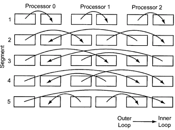
Interleaved Parallelization
The
interleaved
parallelization attemptsto
maintain all ofthe
constraints ofuniprocessor
SVM
training
whiledistributing
the task
of vector optimizationto
multipleprocessors.
The
entire sample setis loaded
onto all n processorsparticipating
in
the
training
process andlogically
subdividedinto 2n
segments,
sothat
each processorcontains
two
segments of sample vectors.To
ensurethe
possibility that any
supportProcessor
1
c
E
0) CO
Figure
3.1-Optimization
pattern
for
two
way
parallelinterleaved
approachProcessor 1
Processor
2
Outer
_Loop
Inner
[image:35.506.151.346.92.240.2]Loop
Figure 3.2
-Optimization
patternfor
three
way
parallelinterleaved
approachThe
optimization pattern specifies which segments on each processor arepermitted
to
optimize at a given stageduring
the
system's operation.As
all ofthe
segments are on all of
the processors, this
selectionis
arbitrary
but
sequencedspecifically
[image:35.506.103.391.299.513.2]optimization sequence
starts,
the
bias,
Lagrange
multipliers,
and error cache areidentical
across all of
the
processors.Each
processorbegins
to
runthe
SMO
algorithm onits
assigned
segments,
looping
untilboth
convergeto
a solution.During
these
optimizationsteps,
the
Lagrange
multipliers and error cache are updatedonly
for
the
segments underconsideration.
After
each processor's sethas
convergedto
alocal
solution,
the
results aredisseminated.
Each
processor sendsits
newLagrange
multipliersto
every
otherprocessor,
sothe
results ofthe
optimizations are availableto the
entire system.The local
bias
values are averagedusing
aMPI
allgatheroperation,
which computesthe
arithmeticmean of all
local bias
valuesto
produce a globalbias for
the
system's subsequentcalculations.
The
optimization process continues sothat
each segmentis
jointly
optimizedwith
every
other segment.In
a2
processorsystem,
this
requires3
optimizationsteps,
while a3
processor system requires5
steps.After
all possible segmentoptimization permutations
have been
performed, the
systemis
examinedfor
termination
conditions.
To
determine if
the
systemhas
completely
convergedto
an appropriatesolution,
the
number of changed multipliersduring
eachstep is
summedfor
the
entiresystem.
If
no multipliershave
changed, then the
algorithmterminates.
If any
multiplierschanged, then the
communication sequencebegins
again.3.2
Blocked Independent Parallelization
While
providing
a general all-to-all optimizationpattern,
the
interleaved
parallelization
increases,
the
number of communication exchangesincreases,
and eachexchange requires
the
immediate
time-consuming
recalculation ofthe
SMO
error cache.These
factors indicate
that the
interleaved
parallelizationmay
be
counterproductive,
asincreasing
parallelizationdramatically
increases
the
computational workload requiredto
continue
the
algorithm'sbasic
operation.In
ord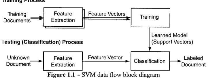
![Figure 2.1Once the separating- Separating hyperplanes in a linear SVM [2] hyperplane has been identified, any given sample with feature vector](https://thumb-us.123doks.com/thumbv2/123dok_us/121233.11697/21.506.89.395.185.405/figure-separating-separating-hyperplanes-linear-hyperplane-identified-feature.webp)
![Figure 2.2- Constraints for optimizing two Lagrange multipliers [12, p. 6]](https://thumb-us.123doks.com/thumbv2/123dok_us/121233.11697/26.506.99.398.185.312/figure-constraints-optimizing-lagrange-multipliers-p.webp)