Development of a linear version of the CIECAM97s chromatic adaptation transform

Rochester Institute of Technology

RIT Scholar Works

Theses Thesis/Dissertation Collections

2000

Development of a linear version of the

CIECAM97s chromatic adaptation transform

Matthew Ochs

Follow this and additional works at:http://scholarworks.rit.edu/theses

This Thesis is brought to you for free and open access by the Thesis/Dissertation Collections at RIT Scholar Works. It has been accepted for inclusion in Theses by an authorized administrator of RIT Scholar Works. For more information, please [email protected].

Recommended Citation

Title Page http://www.cis.rit.edu/research/thesis/bs/2000/ochs/title.html

SIMG-503 Senior Research

Development of a Linear Version of the CIECAM97s

Chromatic Adaptation Transform

Final Report

Matthew J. Ochs Center for Imaging Science Rochester Institute of Technology

May 2000

contents http://www.cis.rit.edu/research/thesis/bs/2000/ochs/contents.html

Development of a Linear Version of the CIECAM97s Chromatic

Adaptation Transform

Matthew J. Ochs

Table of Contents

Abstract

Copyright

Introduction and Background

Theory

CIE L*a*b* Δ E*₉₄

Methods

Generation of Test Data

Implementation of Bradford Model

Development and Implementation of Optimization Technique for Linear Model

Results

Discussion

Conclusions

References

Abstract http://www.cis.rit.edu/research/thesis/bs/2000/ochs/abstract.html

Development of a Linear Version of the CIECAM97s Chromatic Adaptation

Transform

Matthew J. Ochs

Abstract

Color appearance models are used to predict the perceived color of a source. Within these models are

chromatic-adaptation transforms that predict matches only across different viewing conditions. They ignore many of the factors that are used later on in a model. This project was performed to create a simpler and easier to use

chromatic-adaptation transform that was also a linear transform. This was based on the previously known CIECAM97s color appearance model and the non-linear chromatic-adaptation transform that it utilized. The research specifically attempted to create a new transform that will go from XYZ to RGB coordinates that will allow a chromatic adaptation model to perform as well as the Bradford model in CIECAM97s, but while using the linear von Kries rules. A new transform was found, but it can be concluded that it did not perform as well as the CIECAM97s transform.

Copyright http://www.cis.rit.edu/research/thesis/bs/2000/ochs/copyright.html

Copyright © 2000

Center for Imaging Science

Rochester Institute of Technology

Rochester, NY 14623-5604

This work is copyrighted and may not be reproduced in whole or part without permission of the Center for Imaging Science at the Rochester Institute of Technology.

This report is accepted in partial fulfillment of the requirements of the course SIMG-503 Senior Research.

Title: Development of a Linear Version of the CIECAM97s Chromatic Adaptation Transform Author: Matthew J. Ochs

Project Advisor: Mark D. Fairchild SIMG 503 Instructor: Joseph P. Hornak

Thesis http://www.cis.rit.edu/research/thesis/bs/2000/ochs/thesis.htm#I.0

Development of a Linear Version of the CIECAM97s Color Appearance

Model

Matthew J. Ochs

Introduction & Background

Chromatic adaptation is the human visual system’s capability to adjust to widely varying colors of illumination in order to approximately preserve the appearance of object colors. It is the largely independent sensiti

regulation of the mechanisms of color vision. (1)

An example of this is viewing an object with a tungsten light source and also viewing it in daylight. Huma would not see much change in the color with these different illuminations. If a photograph were made of th object in these two conditions, they would end up looking different. The picture taken with the tungsten li source would look yellowish, instead of the bluish tint in daylight. This is due to the fact that film does not have the ability to adjust to the different conditions like humans do.

The data used when studying chromatic adaptation is obtained from corresponding-colors data. Correspon colors are two stimuli, when viewed under different conditions, appear to be the same color. An example of

this is the tristimulus values of one object, XYZ1, viewed in one set of conditions, might seem to b

approximately the same as a second set of tristimulus values, XYZ2, under another, different set of viewing

conditions. These two sets of tristimulus values are referred to as corresponding colors. Information abou viewing conditions of each must also be included with each respective set of tristimulus values. Although the two might appear to be the same, they usually do not have the same numerical values. (1)

The transformation from XYZ1 to XYZ2

is done using a chromatic adaptation model or chromatic adaptation transform. These models do not information about lightness, chroma, or hue. The chromatic adaptation model can now be used corresponding-colors data. Instead of visually recording the data under a second set of viewing conditions, input the values for the first viewing condition into the model, and depending on how good the model is, and the output should be an accurate prediction of the second set of tristimulus values.

A general form of a model can be described using the following equations:

La=f(L,…) (1)

Ma=f(M, …) (2)

Sa=f(S, …) (3)

This model will just predict the three cone signals La, Ma, and Sa (for long, medium, and short) after the effects

of adaptation have acted upon the initial L, M, S

and well as various other factors. A chromatic-adaptation model can be converted to a chromatic-adapt transform by using the forward model for one set of viewing conditions and the inverse of the second set viewing conditions. This is usually done in terms of CIE (International Commission on Illumination) tristimulus values:

XYZ2=f(XYZ1, …) (4)

Thesis http://www.cis.rit.edu/research/thesis/bs/2000/ochs/thesis.htm#I.0

green, and blue). This can be done by a linear transformation (3 x 3 matrix). This is used in chromatic-adaptation and color appearance models that use CIE colorimetry.

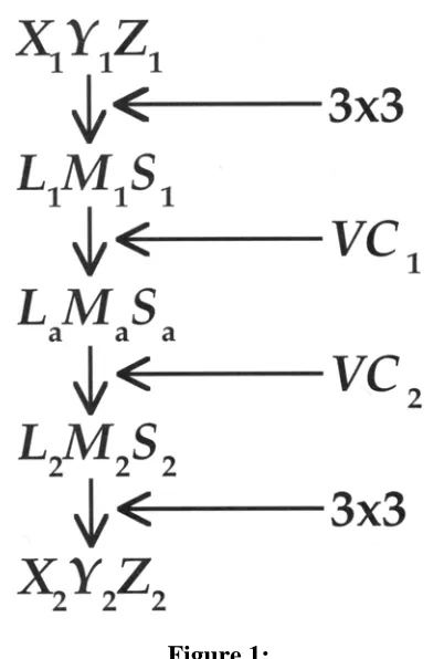
Using these pieces, a generic chromatic-adaptation transform can be made. Starting with CIE tristimulus values for the initial viewing condition, transform these values to cone excitations. Taking into account the various effects of the viewing conditions, use the chromatic-adaptation model to predict the adapted cone signals. Now invert the process by taking the second set of viewing conditions to determine the corresponding colors in terms of cone signals. Finally convert these signals to CIE tristimulus values. This is shown in the following figure:

Figure 1:

A flow chart of the application of a chromatic-adaptation model to the calculation of corresponding colors. (1)

In CIECAM97s (CIE Color Appearance Model, 1997), a Bradford chromatic adaptation model was used with a few modifications. The key parts of the model are that it has a nonlinearity (exponent) on the blue, or short, response and uses a unique matrix transformation to go from XYZ to RGB (or LMS). There is also a D factor that was set to one. The classic model of chromatic adaptation is called a von Kries model. This just transforms

XYZ values to RGB

and then normalizes the result by a white stimulus. This is done by a linear calculation and works well. The changes in the Bradford model seem to improve on this though.(2)

Theory

Thesis http://www.cis.rit.edu/research/thesis/bs/2000/ochs/thesis.htm#I.0

Since the color temperature of daylight changes constantly, a mean daylight has been standardized at 6500K This is what D65 refers to; a standard illuminant at 6500K. (3) CIELAB was created in 1976 in an attempt to

promote uniformity in calculating color differences. To calculate CIELAB coordinates, start with the two sets of CIE XYZ tristimulus values provided. One of these is for a stimulus and the other is for a reference, Xn, Yn,

Zn. Normalize these to those of the white by dividing the stimulus values by the reference values. These

adapted signals are then subjected to a compressive nonlinearity represented by a cube root in the CIE equations. These signals are then combined into three response dimensions of the opponent-colors theory o color vision. Finally, proper constants are used in the equations that will provide the required perceptual spacing and proper relationship between the three dimensions. This entire process is shown in the follo equations:

L*=f(Y/Yn)-16 (5)

a*=500[f(X/Xn)-f(Y/Yn)] (6)

b*=200[f(Y/Yn)-f(Z/Zn)] (7)

f(ω )=(ω )1/3ω >0.008856 (8)

f(ω )=7.787(ω )+16/116 ω≤ 0.008856 (9)

L* represents lightness, a* approximates redness-greenness, and b* approximates yellowness-blueness. This will represent the data in Cartesian coordinates to form a three dimensional space. This can be also represented in terms of cylindrical coordinates that will predict chroma, C*ab, and hue, hab.

C*ab=√ (a*2+b*2) (10)

hab=tan-1(b*/a*) (11)

Thesis http://www.cis.rit.edu/research/thesis/bs/2000/ochs/thesis.htm#I.0

Δ

E*

Δ E*94

is a color-difference calculation based upon the Euclidean distance between the color of a sample under test

and reference sources. The Δ E*94 is a simplified version of an earlier Δ E formula. The equations used to

calculate this are:

ΔE*94=[(Δ L*/kLSL)2+(Δ C*ab/kCSC)2+(Δ H*ab/kHSH)2]1/2 (12)

SL = 1 (13)

Sc = 1+ 0.045C*ab (14)

SH = 1+0.015C*ab (15)

C*ab is referring to the CIELAB chroma of the color difference pair. The kL, kC, and kH are used to offset any

experimental variables and may be set to 1 under defined reference conditions. (1)

Methods

Generation of Test Data Set

The first step in the procedure of this project was to obtain a data set to test the models with. This was obtained from the Munsell Book of Color samples from Dave Wyble's work. (4) Three seperate data sets were tested. The first was the colors that physically appeared in the 1929 Munsell Book of Color. The second being real colors only, "real" being those lying inside the Macadam limits. The third data set used all the Munsell data, including extrapolated colors. Note that extrapolated colors are in some cases unreal. That is, some lie outsize the Macadam limits. (5) This gave data for the x and y chromaticity values as well as the Y tristimulus value. To find the X and Z tristimulus values, the following equations were used:

(16)

(17)

Now a data set of XYZ

values are known which were used as input into the CIECAM97s and linear models. These were read into an IDL program that was written to perform the following calculations.

Implementation of Bradford Model

Thesis http://www.cis.rit.edu/research/thesis/bs/2000/ochs/thesis.htm#I.0

(18)

(19)

The difference between the von Kries and the CIECAM97s transform that follows is an exponential

nonlinearity on the B, or S signal. This exponential is what this project was trying to eliminate. The D, which describes the degree of adaptation, in the following transformation was always set to 1 for all work in this project.

Rc=[D(1.0/Rw)+1-D]R (20)

Gc=[D(1.0/Gw)+1-D]G (21)

Bc=[D(1.0/Bwp)+1-D]|B|p (22)

p=(Bw/1.0)0.0834 (23)

These new RGB values were then transformed back to a set of XYZ values that are the output of the Bradford model.

(24)

Development and Implementation of Optimization Technique for Linear Model

Now that data from the Bradford model was known, a new linear model was created to give similar results. The general for this is:

(25)

The A matrices are linear and diagonal. Each one can be represented as:

Thesis http://www.cis.rit.edu/research/thesis/bs/2000/ochs/thesis.htm#I.0

(27)

Since the nonlinearity of the Bradford model is no longer present, the M chromatic adaptation transform matrix needed to be changed in order to get XYZ

values that were similar to those found previously. This M matrix was found using the AMOEBA function in IDL. The AMOEBA function performs multidimensional minimization of a function using the downhill simplex method. This function altered the values of the Bradford M matrix for a number of iterations and found a new M matrix that when utilized in the linear model, would give data similar to the output XYZ values from the Bradford model. This routine is written into the IDL language. Once this routine returned the values for the new matrix, the new values were implemented into the linear model. A new set of XYZ from the linear model was then calculated. Now that there is a set of XYZ values from both the CIECAM97s model and the linear model, the accuracy of the model was evaluated. To do this, the XYZ values were converted to CIE L*a*b* values for both models, and the Δ E*94 was then calculated to compare the two.

For comparison, three matrices were tested along with the new matrix found using the AMOEBA function. The first two come from personal communications with my advisor. The third is just the average of these two. These resulted from research whose goal was similar to this project. The three matrices are:

Thesis http://www.cis.rit.edu/research/thesis/bs/2000/ochs/thesis.htm#I.0

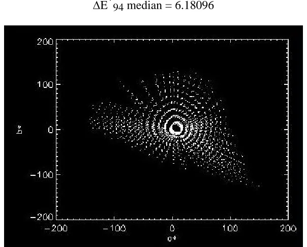
Figure 3: Output data from Bradford model using 1929 Munsell data

This is the new M matrix that was found using the AMOEBA function in IDL and the 1929 Munsell data.

Thesis http://www.cis.rit.edu/research/thesis/bs/2000/ochs/thesis.htm#I.0

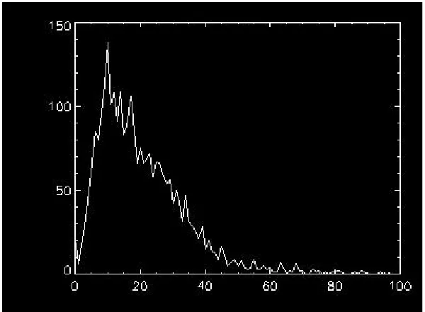
Figure 5: Histogram of Δ E*94 values using 1929 Munsell data

ΔE*94 data from 1929 Munsell data.

ΔE*94 min = 0.670628

ΔE*94 mean = 6.90528

ΔE*94 max = 25.1795

ΔE*94 median = 6.18096

Figure 6: Output data from Bradford Model using real Munsell data

Thesis http://www.cis.rit.edu/research/thesis/bs/2000/ochs/thesis.htm#I.0

Figure 7: Output data from linear model using real Munsell data

Figure 8: Histogram of Δ E*94 values using real Munsell data

Δ E*94 min = 0.391057

Δ E*94 mean = 21.2884

Δ E*94 max = 98.0225

Thesis http://www.cis.rit.edu/research/thesis/bs/2000/ochs/thesis.htm#I.0

Figure 9: Output data from Bradford model using all Munsell data

The following Δ E*94

data is for the "mystery" matrix, the "derby" matrix, and the average of these two, respectively.

Δ E*94 min = 0.603249

Δ E*94 mean = 11.4141

Δ E*94 max = 47.3711

Δ E*94 median = 9.86326

Δ E*94 min = 0.542887

Δ E*94 mean = 12.0115

Δ E*94 max = 49.7402

Δ E*94 median = 10.3158

Δ E*94 min = 0.486392

Δ E*94 mean = 11.9741

Δ E*94 max = 48.2328

Thesis http://www.cis.rit.edu/research/thesis/bs/2000/ochs/thesis.htm#I.0

Discussion

The graphs that resulted from the Bradford model and the linear model give a visual comparison of the two models. There are obvious similarities between the two, but the accuracy of the two can be examined further. At best, the new transform that was found using the 1929 Munsell data had a mean of 6.90528 which is on the border of acceptability. The visual uncertainty for such determinations is about 4 units. Thus, the disagreement between the models is significant. However, it might be biased by some very large errors for colors that have never really been studied experimentally. This would explain the maximum of 25.1795 as well as the presence of other high values in the histogram. This may also be pulling the mean to such a high value. It is good to note that most of the Δ E*94 occur at lower values, but still not in the range that was expected.

When using the real Munsell values, the presence of more extreme colors created less accurate data. When all of the Munsell data was used, a new optimized transform could not even be found due to the extremity of the colors. It may be useful to try other data sets as input or to try to eliminate some of the colors that have not been studied previously. This may result in a better transform, but as the data set is truncated, it may be less reliable over a larger gamut of colors. The optimized transform found using the 1929 data resulted in a better fit than when using the two matrices provided by Fairchild and averaged matrix. This is better for these particular data, but that's to be expected since it was fit to the 1929 data, and the data set for the others was different. It works better for what has been tested so far, but further independent tests would be required to make a robust conclusion..

Conclusions

The hypothesis for this research project was that a new transform from XYZ to RGB coordinates should be obtained that will allow a chromatic adaptation model to perform as well as the Bradford model in

CIECAM97s, but while using the linear von Kries rules. Although a new linear transform was found, it did not perform as accurately as the Bradford model.

References http://www.cis.rit.edu/research/thesis/bs/2000/ochs/references.html

Development of a Linear Version of the CIECAM97s Chromatic

Adaptation Transform

Matthew J. Ochs

References

Fairchild, Mark D. (1998). Color Appearance Models. Reading, Mass: Addison Wesley Longman, Inc.

1.

CIE TCI-34. (1998). The CIE Interim Colour Appearance Model (Simple Version), CIECAM97s.

2.

Berger-Schunn, Anni. (1994). Practical Color Measurement: A Primer for the Beginner. A Reminder for the Expert. New York: Wiley -Interscience Publication.

3.

Wyble, David R. & Fairchild, Mark D. (2000). Prediction of Munsell Appearance Scales Using Various Color Appearance Models. Color Research & Application, first quarter 2000.

4.

Munsell Renotation Data. URL: http://www.cis.rit.edu/mcsl/online/munsell.shtml Dave Wyble. Rochester Institute of Technology. October 16, 1999.

5.