City, University of London Institutional Repository
Citation
:
Rosti, M. E., Omidyeganeh, M. & Pinelli, A. (2018). Passive control of the flow around unsteady aerofoils using a self-activated deployable flap. Journal of Turbulence, 19(3), pp. 204-228. doi: 10.1080/14685248.2017.1314486This is the accepted version of the paper.
This version of the publication may differ from the final published
version.
Permanent repository link:
http://openaccess.city.ac.uk/17323/Link to published version
:
http://dx.doi.org/10.1080/14685248.2017.1314486Copyright and reuse:
City Research Online aims to make research
outputs of City, University of London available to a wider audience.
Copyright and Moral Rights remain with the author(s) and/or copyright
holders. URLs from City Research Online may be freely distributed and
linked to.
City Research Online: http://openaccess.city.ac.uk/ [email protected]
Journal of Turbulence Vol. 00, No. 00, 200x, 1–18
RESEARCH ARTICLE
Passive control of the flow around unsteady aerofoils using a self-activated deployable flap
Marco E. Rosti∗, Mohammad Omidyeganeh, Alfredo Pinelli
Department of Mechanical and Aeronautical Engineering City University London
London, U.K.
(Received 00 Month 200x; final version received 00 Month 200x)
Self-activated feathers are used by many birds to adapt their wing characteristics to the sud-den change of flight incisud-dence angle (e.g., sudsud-den increase in angle of attack due to gusts or perching manoeuvres). In particular, dorsal feathers are believed to pop up as a conse-quence of unsteady flow separation and to interact with the flow to palliate the sudden stall breakdown typical of dynamic stall. Inspired by the adaptive character of birds feathers, some authors have envisaged the potential benefits of using of flexible flaps mounted on aerody-namic surfaces to counteract the negative aerodyaerody-namic effects associated with dyaerody-namic stall. This contribution explores more in depth the physical mechanisms that play a role in the modification of the unsteady flow field generated by a NACA0020 aerofoil equipped with an elastically mounted flap undergoing a specific ramp-up manoeuvre. It is found that it is possible to design flaps that limit the severity of the dynamic stall breakdown by increasing the value of the lift overshoot also smoothing its abrupt decay in time. A detailed analysis on the modification of the unsteady vorticity field due to the flap flow interaction during the ramp-up motion is also provided to explain the more benign aerodynamic response obtained when the flap is in use.
1. Introduction
The demand for helicopters with increased performance and the quest for efficiency improvements in vertical axis wind turbines have prompted further investigations into the dynamic stall that often appears on rotors retreating blades. Dynamic stall is an unsteady phenomenon that takes place on lifting objects in response to time variations of the angle of attack, and it is responsible for dramatic changes in the aerodynamic loads, high vibration affecting the dynamic performance, and occur-rence of aeroelastic instability (stall flutter). A considerable number of researches have extensively studied these phenomena in the past [1–6]. Experimental works have mainly focused on unsteady flows over two-dimensional aerofoils undergoing prescribed pitching motions [1–5, 7–11]. McCroskey [2, 3] discovered that the stall is characterised by a lift overshoot, due to the passage of a large scale vortex over the suction side of the aerofoil, followed by a lift breakdown associated with the vortex detachment, and Shih et al. [12] suggested that the main stall vortex is in-duced by the early boundary layer separation near the leading-edge of the aerofoil, and that full stall occurs when the boundary layer detaches completely from the aerofoil.
High fidelity numerical simulations of dynamic stall in configuration of aeronau-tical interest are particularly expensive due to the broad range of time and space
∗Corresponding author. Email: [email protected]
ISSN: 1468-5248 (online only) c
200x Taylor & Francis
scales involved in the phenomenon. However, conventional turbulence models are known to fail in producing reliable solutions in such complex, out of equilibrium conditions: unsteady, recirculating and locally transitional flow. A general, but somehow outdated review on the numerical simulations of dynamic stall [13–19] can be found in the work of Ekaterinaris and Platzer [20]. Several other works have highlighted the difficulties that RANS calculations encounter when dealing with dynamic stall. In particular, Wang et al. [17] used two variants of thek−ωmodel, the standard and the SST one, to simulate the flow at moderate high Reynolds number Rec = 105. From a comparison with experimental results, they noticed
that the models can not precisely capture the size and position of the dynamic stall vortex. Moreover, the quality of the predictions of the models deteriorate as the angle of attack increases. Dumlupinar and Murthy [18] further investigated the performances of various turbulence models and pointed out that different tur-bulence closures predict a broad range of different behaviours even in light stall cases. Recently, Rosti et al. [21] performed a DNS of flow around a NACA0020 aerofoil, with the aim of elucidating the physical mechanisms that determine the dynamic stall vortex creation, its evolution along the aerofoil and the subsequent detachment.
Because of the undesirable aerodynamic and structural consequences of dynamic stall, many researchers have focused on the development of control techniques able to palliate such adverse effects. In this framework, a number of different passive and active control techniques [22–25] have been proposed in the past. More recently, researchers have been looking at biomimetic devices to control flow separation on aerofoils at high angle of attack. In particular, it has been observed that birds can overcome certain flight critical conditions, by popping up some of their feathers when flow separation starts to develop on the upper side of their wing [26–28]. It is believed that the feathers lift up may contain backflow thus preventing an abrupt breakdown of aerofoil lift typical of dynamic stall. With the aim of demonstrating the effectiveness of devices mimicking the feathers pop-up, Schatz et al. [29] have shown that a self-activated spanwise flap elastically mounted by the trailing edge of an aerofoil can enhance lift by more than 10% at a chord Reynolds number
Rec=U∞c/ν (U∞ being the magnitude of the free stream velocity, c the aerofoil
chord andν the kinematic viscosity) in the range of 106. In a related experiment, Schluter [30] has also demonstrated that dynamic stall lift-breakdown is less severe when a similar flap is used.
More recently, Bruecker and Weidner [6] used hairy flaps (i.e., flaps with a thick-ness much smaller than the plant form sizes) to manipulate the dynamic stall of a wing at moderate Reynolds numberRec= 77000, observing a delay of the dynamic
stall. The authors claim that the delay is achieved by both the reduction of the backflow, and by regularising of the shear layer roll-up process. Moreover, they suggest that the onset of the shear layer non-linear growth is delayed via mode-locking of the fundamental instability mode with the motion of the flaps. Rosti et al. [31, 32] performed a DNS of the flow around a NACA0020 aerofoil with a flap mounted via a torsional spring on its suction side at a fixed angle of attack 20o.
U∞ α outlet inlet x y z (a)
L
c
y xFigure 1. (a) Sketch of the computational domain. (b) Grid in the proximity of the aerofoil (nodes are plotted with a skip index of six). The inserted figure is an enlargement of the area surrounding the trailing edge. (c) Sketch of the flap hinged on the suction side of the aerofoil through a torsional spring.
activated.
In the present work we focus on the passive control of a NACA0020 aerofoil undergoing a ramp-up manoeuvre (angle of attack increased linearly in time from 0o to 20o degrees at an angular speed of 0.12U∞/c), using self-adaptive flaplets elastically mounted on its suction side. The next section introduces the numerical formulation and the problem setup. In the following one, we present our original contribution by offering an exhaustive analysis of the flow during a ramp-up motion atRec= 2×10⁴. Finally, the last section summarizes our main findings and draws
some conclusions.
2. Numerical formulation
To tackle the problem at hand, we consider an incompressible three-dimensional unsteady flow field, around a straight wing with an infinite spanwise dimension as sketched in Figure (1a). The chosen coordinate system is a Cartesian inertial one, with the x and y axis (x1 and x2) aligned with the parallel and normal to
the aerofoil chord directions, whilez (x3) is the axis normal to the paper. Also,u,
v and w (u1,u2 and u3) are used to denote the velocity components parallel and
normal to the chord, and along the span respectively. With the given notations, using Einstein’s summation convention, the dimensionless equations that govern the incompressible flow motion are:
∂ui
∂t + ∂uiuj
∂xj
=−∂P
∂xi
+ 1
Rec
∂2ui
∂xj∂xj
+fi, (1)
∂ui
∂xi
= 0, (2)
The equations given above, have been made non-dimensional using the magnitude of the free stream velocity U∞ and the aerofoil chord c. Also, in the momentum Equation (1),Rec=U∞c/ν is the chord-based Reynolds number and firepresents
a system of singular body forces used to keep into account the presence of the flap as it will be discussed later.
[image:4.595.86.455.54.158.2]employed for all the other terms. The pressure Poisson equation arising when im-posing the solenoidal condition on the velocity field, is transformed into a series of two-dimensional Helmholtz equations in wave number space via Fast Fourier transform (FFT) in the spanwise direction. Each of the resultant elliptic 2D prob-lem is then solved using a preconditioned Krylov method (PETSc library [37]). In particular, the iterative Biconjugate Gradient Stabilized (BiCGStab) method pre-conditioned by an algebraic multigrid preconditioner (boomerAMG) [38] revealed to be quite efficient in dealing with the decoupled elliptic problems. The code is parallelized using a streamwise domain decomposition via the MPI message passing library. Further details on the code, its parallelization and the extensive validation campaign that has been carried out in the past can be found in Rosti et al. [21].
The aerofoil that has been selected for the present study is a symmetric NACA0020, which has been extensively studied in static stalled conditions by the authors in a previous research [21]. The flow domain around the aerofoil is meshed using a body fitted C grid arrangement (see Figure (1b)). The grid is adapted to the three dimensional case by uniformly repeating the baseline 2Dgrid in the span-wise direction. The boundary conditions that have been considered are as follows. Impermeability and no slip conditions are set on the aerofoil wall, periodic condi-tions are enforced on the planes bounding the domain in the spanwise direction, and continuity of the flow variables is applied through the top and bottom planes generated by the C-grid topology downstream of the trailing edge. On the external surface that bounds the computational domain, a convective boundary condition is used for the outlet, while a Dirichlet type condition based on an far-filed irrota-tional approximation (Hess and Smith panel method [39]) of the flow is enforced on the inlet portion of the surface bounding the computational domain.
When a dynamic variation of the angle of incidence is considered, as in the a ramp-up case, the inlet conditions are modified accordingly by changing the local direction of the velocity vector. An alternative formulation to impose the ramp-up manoeuvre, consisting in rotating the aerofoil in time using a non-inertial frame of reference mounted on the wing [40] (axis of rotation passing through the centroid of the foil), has also been considered. Before discarding this last option, we have evaluated the difference in the results obtained when using the two approaches. No significant differences have been observed when low reduced frequencies are considered and the rotation takes place along an axis normal to the paper passing through the centroid of the aerofoil. In particular, the variation in the lift and drag integral values revealed to be quite marginal.
Thus, all the three-dimensional simulations that will be presented have been obtained considering an inertial frame of reference, at a chord Reynolds number
Rec = 20000 and by varying the angle of attack according to a ramp function of
time with an initial linear increase (constant rate k = 0.12U∞/c) from 0 to 20o and a subsequent constant value of the angle of attack, kept at α = 20o (stalled condition).
The grid system that has been chosen for the three-dimensional simulations, has been determined after a number of trial-and-error tests and companion grid con-vergence studies spanning the whole free stream velocity vector rotation. Finally, we have selected a 2785×626×97 (nodes in thex1,x2 and x3 directions,
respec-tively) grid. In terms of local wall units, in the turbulent portion of the attached boundary layer, the corresponding mesh resolution verifies ∆x+<3.0, ∆y+<0.5 and ∆z+ <7.5 (superscript + indicates standard local viscous units lengths: i.e., lengths made non dimensional using the kinematic viscosityν, and the skin friction velocity uτ). Further details on the procedure that has been followed to generate
The conceptual aerofoil-flap configuration that has been considered is sketched in Figure (1c) showing the NACA0020 aerofoil with a rigid thin flap hinged via a torsional spring in the trailing edge region. The flap motion takes place in thex-y
plane (i.e., no torsion allowed around their main axis), and is modelled using the second order ordinary differential equation
Iθ¨+Cθ˙+Kθ=T (3)
In equation (3),θis the angular displacement with respect to the equilibrium angle (i.e,θ= 0) assumed to correspond to the condition in which the flap is tangent to the aerofoil. Also,I is the flap moment of inertia,C andK are the spring damping factor and stiffness, whileT is the torque exerted by the fluid on the flap.
The fluid-solid coupling of the moving appendages is kept into account by a singular body force distribution discretely applied along the flaps. This discrete, localised force system corresponds to the forces fi appearing in the momentum
equation (Equation (1)), and the integral of their moments about the flap hinge constitutes the torque termT in (3). The intensity of the body forcesfiis related to
the correct imposition of zero relative fluid velocity on the flaps. In particular, their values are determined by the immersed-boundary RKPM method [41] supposing a zero thickness flap. Further details on the implementation of the present fluid-structure interaction methodology using the IB-RKPM method on moving and/or deformable slender bodies are given in Favier et al. [42].
3. Results and discussions
To introduce the effects produced by the presence of a membrane-like flap hinged on the suction side of an aerofoil, we first illustrate the main features of the baseline flow under consideration: the flow around a NACA0020 aerofoil undergoing a ramp-up manoeuvre without the application of any control device at a chord Reynolds number fixed to the value of Rec = 2×10⁴. In particular, the angle of attack
undergoes an initial linear increase fromα= 0 toα = 20owith a reduced frequency
k= 0.12U∞/c followed by a steady value of the angle atα= 20o. The variation of
α with time matches the experimental conditions of Brucker and Weidner [6] and is also very similar to the one considered in [5].
3.1. Baseline flow description
All the ramp-up simulations are initialized from a fully developed, zero degree angle of attack flow condition. All averaged quantities that will be presented have been obtained employing a double averaging procedure: space averaging in the homogeneousz-direction and ensemble averaging at same time instants obtained from simulations using different initial conditions. In particular, similarly to Rosti et al. [21], we have considered ten realisations obtained using ten different initial conditions obtained from instantaneous zero degree flow fields sampled within two shedding cycles.
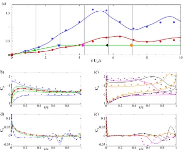
Figure 2. (a) Lift (blue line) and drag (red line) coefficients as a function of time. The green line is representative of the time variation of the angle of attack. Along this last line, the symbols indicate 6 particular time instants for which integral quantities along the aerofoil are represented in the remaining panels of the figure. In these diagrams, solid continuous lines represent the baseline cases while the symbols are for the cases of the aerofoil equipped with the flap. Also the colours indicate the time level at which the information has been extracted (consistently with the colours of the symbols of the top panel). (b)-(c) Pressure coefficientCpand (d)-(e) friction coefficientCf at the selected times.
is related to the detachment of the dynamic stall vortex from the aerofoil. At a later time, the integral forces oscillate slowly converging towards the asymptotic static-stall values, in agreement with the physical description given by McCroskey [2]. During their time evolution, the maximum values achieved by the lift and drag coefficients areCL= 1.58 andCD = 0.67, respectively. Both these values are about
the double of the corresponding coefficients measured in the static case atα = 20o (see Rosti et al. [21]).
The other panels of Figure (2) show the time evolution of the pressure coeffi-cientsCp (b and c) and of the friction coefficients Cf (d and e). Figure (3) displays
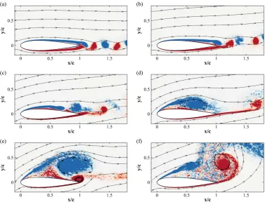
the contours of the span-wise,z-component of vorticity ωz, averaged in the
homo-geneousz-direction at the same six times as the ones considered in Figure (2). In particular, the first plot corresponds to the zero degree angle of attack, the second toα = 10o and the others at various time instants at α= 20o. Figure (3a) shows how the flow is mostly symmetric over the aerofoil surface when α = 0o. Con-sistently, also the Cp distribution appears to be symmetric (Figure (2b)), with a
[image:7.595.88.463.53.360.2]Figure 3. Contour plots of the space and ensemble average of the spanwise component of vorticityωz of
the baseline simulation. The contours plots have been obtained at the times indicated in Figure (2a). Blue negative vorticity, red positive (±7U∞/c).
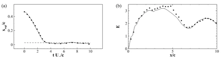
separation point move towards the leading edge (Figure (2d)). Even after having reached the maximum incidence, the lift coefficient keeps increasing (Figure (2a)) with a pressure coefficient distribution that does not show the typical separation plateau [21]. As the peak of the pressure near the leading-edge is still increasing, and a second peak appears around the mid-chord (Figure (2c)). The latter is the footprint of a large vortex which has started to form on the suction side (i.e., the so called dynamic stall vortex), see Figure (3d). It is also noted that until the maximum lift is not reached, no vortices are shed from the trailing edge as can be educed from Figure (3d). After its formation, the dynamic stall vortex is con-vected downstream towards the trailing edge (as indicated by the displacement of the second pressure peak in Figure (2c)), where an induced counter rotating vortex is formed, see Figure (3e). When the dynamic stall vortex finally detaches from the aerofoil and the trailing edge vortex reaches its maximum size (Figure (3f)), the pressure attains an almost constant distribution indicating a fully separated flow condition (Figure (2c)). The complete time evolution of the separation point is re-ported by the solid line in Figure (4a). At α = 0o the separation point is located atxs= 0.47c, moving towards the leading edge as the angle of attack is increased.
As already remarked, the static stall separation point xs = 0.025c (dashed line)
[image:8.595.86.464.50.338.2]Figure 4. Time evolutions of the (a) downstream separation point and (b) aerodynamic efficiencyE =
CL/CD during the ramp-up manoeuvre. Solid lines and symbols are used for the baseline and controlled
cases, respectively. The dashed line in (a) represents the separation point at 20o.
3.2. Hinged flap: parametric study
We now turn our attention to the effects of a membrane-like flap mounted on the suction side of the aerofoil during the same ramp-up motion. As an initial step, we had to identify a design of the flap able to deliver substantial aerodynamic benefits during the manoeuvre. A proper design must keep into account that the flap motion and its effects on the flow field are controlled by various parameters, such as its length, inertia, position, the torsional spring stiffness and its damping factor. In a previous study, focusing on stall at fixed angle of attack (atα= 20o), we have carried out a parametric study aimed to identify an optimal control condition defined as the one that delivers the highest lift coefficient CL while preserving
or improving the aerodynamic efficiency E = CL/CD (see [32]). For the present
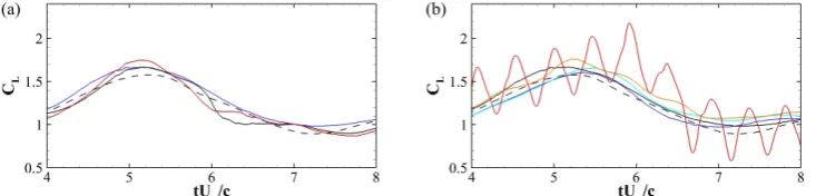
study, where the incidence varies with time, we proceed with a similar parametric study but pursuing a different aerodynamic condition. In particular, we define as a desired condition the one that maintains high efficiency during all the manoeuvre, postpones the dynamic stall, i.e., the lift breakdown, and reduces the subsequent degradation rate of the lift coefficient. Tablr (1) details all the flap configurations that have been considered. In particular, apart from the baseline case without flap, we have analysed flap lengths in the rangeL/c = 0.1−0.3, and spring stiffnesses in the range K = 0.037−0.600. Note that the spring stiffness can be related to the natural frequency of the flap as K = I(2πf)2, where I is the moment of inertia with respect to the rotation axis given by I =mL2/3, (m being the mass per unit spanwise length). The chosen stiffness values correspond to flap natural frequencies ranging between the half and the double of the shedding frequency of the baseline foil at the maximum angle of attack achieved in the ramp-up motion, i.e.,f0= 0.58U∞/catα= 20o. In previous studies (see [31] and [32]), we have also analysed both the effects of the flap hinge position, and of a different configuration consisting of two flaps positioned in tandem on the suction side of the aerofoil. The effect of these parameters has not been considered in this study, since it was found that the aerodynamic performances were not very sensitive to their introduction. Having considered all the cases reported in Table (1), we have found that the best performance is achieved when using a flap 0.1clong, resonating with the shedding frequency of the uncontrolled aerofoil at an incidence of α = 20o. A summary of the time evolution of the lift coefficients during the ramp-up manoeuvre obtained using various flap configurations is reported in Figure (5) (note that, only the lift breakdown phase is shown in the figure).
3.3. Flow around the foil equipped with the selected flap
[image:9.595.87.456.46.141.2]Case f /f0 L/c xF/c K×103 I×103
Ref − − − − −
[image:10.595.172.390.44.211.2]F0.25-L0.10-X0.7 0.25 0.10 0.7 2.3461 3.3333 F0.50-L0.10-X0.7 0.50 0.10 0.7 9.3847 3.3333 F1.00-L0.10-X0.7 1.00 0.10 0.7 37.539 3.3333 F2.00-L0.10-X0.7 2.00 0.10 0.7 150.15 3.3333 F4.00-L0.10-X0.7 4.00 0.10 0.7 600.62 3.3333 F0.25-L0.20-X0.7 0.25 0.20 0.7 9.3847 13.333 F0.50-L0.20-X0.7 0.50 0.20 0.7 37.539 13.333 F1.00-L0.20-X0.7 1.00 0.20 0.7 150.15 13.333 F2.00-L0.20-X0.7 2.00 0.20 0.7 600.62 13.333 F4.00-L0.20-X0.7 4.00 0.20 0.7 2402.5 13.333 F0.25-L0.30-X0.7 0.25 0.30 0.7 21.115 30.000 F0.50-L0.30-X0.7 0.50 0.30 0.7 84.462 30.000 F1.00-L0.30-X0.7 1.00 0.30 0.7 337.85 30.000 F2.00-L0.30-X0.7 2.00 0.30 0.7 1351.4 30.000 F4.00-L0.30-X0.7 4.00 0.30 0.7 5405.6 30.000
Table 1. Flap configurations considered in the parametric study. The aerofoil is NACA0020 and the Reynolds number isRec= 20000. The flap parameters, i.e., the ratio between the spring natural frequency and the shedding frequencyf /f0, the flap’s lengthL, the hinge positionxF, the spring rotational stiffnessK, and the moment of inertiaIare provided.
Figure 5. Evolution of the liftCL for some of the cases considered in the parametric study. In panel
(a), the length of the flap is varied, while keeping the flap natural frequency equal to the foil shedding frequency. The blue, black and red lines are used to identify the lift coefficients obtained with flap lengths equal toL= 0.1c, 0.2cand 0.3c, respectively. In panel (b) we consider cases where the length of the flap is frozen toL= 0.1c, and the natural frequency of the flap is changed; the blue, light blue, black, orange and red lines are used forf = 0.25f0, 0.5f0, 1.0f0, 2.0f0 and 4.0f0, respectively (f0 being the shedding
frequency of the baseline foil at 20o incidence). The dashed line is used to indicate the reference cases.
chosen flap configuration corresponds to the one delivering the best performances as determined via the parametric campaign described in the previous section: flap length 0.1c, hinged at 0.7c, infinitely long in the spanwise direction, and with a torsional stiffness adjusted to produce a flap natural frequency matchingf0 (the shedding frequency of the baseline profile at 20o incidence). For convenience, in what follows the aerofoil equipped with the aforementioned, quasi-optimal flap will be simply termed either as the controlled aerofoil, or the aerofoil with the flap. A comparison of the time evolution of the lift and drag coefficients of the baseline aerofoil (continuous line) versus the controlled one (dotted line) during the ramp-up motion is displayed in Figure (2). From the diagram, it appears that the drag coefficient CD is only slightly influenced by the presence of the flap,
while the lift coefficientCL is increased during the initial 7tU∞/c time units, thus
indicating an overall increase in aerodynamic efficiency E during the ramp-up motion. Figure (4b) reports the time variations of the aerodynamic efficiency E
(defined as the ratio between the lift and drag coefficients, i.e., E = CL/CD).
[image:10.595.89.456.257.345.2]Figure 6. Contour plots of the space and ensemble average of the spanwise component of vorticityωz
for the controlled case with flap, sampled at the times given in Figure (2a). Blue negative vorticity, red positive (±7U∞/c).
overshoot delivers a smoother aerodynamic response to the unsteady change of incidence. The milder aerodynamic response induced by the presence of the flap is also enhanced by the extended time interval over which the lift decreases after the first lift maximum: in the controlled case this period of time is extended by 5% as compared to the baseline case.
Figure (6) shows the flow evolution during the ramp-up manoeuvre in terms of spatial and phased averaged spanwise vorticity when the flap is in use. The selected snapshots and vorticity levels correspond to the ones of the baseline case illustrated in Figure (3). Initially, at α= 0o, the flow is mostly attached to the aerofoil, and the flaplet lies tangentially on the aerofoil surface (Figure (6a)). As the angle of attack is increased and the separation point moves upstream (Figure (6b-c)), the flap starts to lift reducing the backflow advancing from the trailing edge. Within this stage, the pressure coefficientCp (Figure (2b)) of the controlled case shows a
higher leading edge pressure peak. It is also noted that the presence of the flap postpones the Cf oscillations (see Figure (2d)). In the following stage, when the
dynamic stall vortex is forming and maximum lift is almost reached (Figure (6c-e)), the flap reverses his movement, now directing towards the wing surface. The flap downward motion generates a jet that displaces the forming trailing edge vortex downstream. This flap-flow interaction process delays the detachment of the dy-namic stall vortex, resulting in a higher maximum lift value (maximum value in the controlled case: CLmax = 1.68), and in a milder lift breakdown. A footprint of the same process can also be observed in theCp andCf distributions in Figure (2c,e)
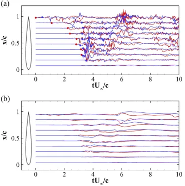
[image:11.595.88.464.41.338.2]Figure 7. Fluctuations of the (a)x-velocity componentsu0 and (b) pressurep as a function of time for various points near the aerofoil surface. For clarity, the fluctuations are shifted according to the chord location where they were measured. Red lines are for the baseline case, blue lines are for the aerofoil with the flap. For further explanations see the text
by the presence of the flap.
When describing Figure (2d-e), we have already highlighted the presence of some oscillations in the Cf distribution by the trailing edge region. These oscillations
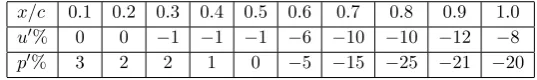
[image:12.595.86.463.56.436.2]x/c 0.1 0.2 0.3 0.4 0.5 0.6 0.7 0.8 0.9 1.0
u0% 0 0 −1 −1 −1 −6 −10 −10 −12 −8
[image:13.595.143.412.48.88.2]p0% 3 2 2 1 0 −5 −15 −25 −21 −20
Table 2. Percentage variations of the r.m.s. values of the streamwise velocity component and pressure fluctuations in the aerofoil with flap with respect to the baseline foil. The locationsx/care the same as the ones Figure (7)
is considered, the situation is quite different. In this case, the locations upstream of the flap hinge are reached by the perturbations with a slight time delay, while the the fluctuations downstream of the hinge are strongly reduced in amplitude and postponed in time. Table (2) confirms the aforementioned effect of the flap in reducing the velocity fluctuations in the rear part of the aerofoil (by approximately 10%) while leaving the intensity of the fluctuations almost unchanged in the front part.
Figure (7b) and Table (2) also illustrate the behaviour of the pressure fluctua-tions that further highlights the difference between the two cases with a maximum reduction of pressure rms of about 25% at 80% of the chord.
Further insight into the physical processes taking place during the ramp-up mo-tion can be gained by analysing the time emergence of coherent structures, their mutual interactions and the generation of the wake. In particular, vortical coherent structures have been identified using theQ-criterion proposed by Hunt et al. [43]. This technique allocates a vortex to all spatial regions that verify the condition
Q= 1 2 |Ω|
2− |S|2
>0, (4)
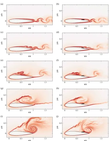
whereS = 12 ∇u+∇uTis the rate of strain tensor andΩ= 12 ∇u−∇uTis the vorticity tensor. InstantaneousQiso-surfaces are shown in Figure (8). The left column corresponds to the baseline profile, while the right one presents the case of the aerofoil with the flap. The rows in the figure have been captured at the same time after the beginning of the ramp-up motion. Panels in the first row (a and b) correspond to the earliest stages att = 1.45c/U∞, when the angle of attack is
α= 10o. The flow is very similar in the two cases presenting a slight asymmetry, with coherent structures generated only past the trailing edge area of the suction side. Atα= 20o(panels c and d), the shear layer rolls-up into a recirculating region that closes at about the mid-chord location. However, the size and intensity of the large roller is strongly reduced when the flap is in use. Moreover in the controlled case, the whole shear layer instability and the consequent roll-up appear to be shifted downstream indicating a time delay in the whole instability process. The next panels (e, f and g and h) show how the roll-up process continues to develop leading to the formation of a very large recirculating zone (i.e., the dynamic stall vortex) that basically covers all the foil suction side. Again, the recirculating region and its intensity seem to be diminished by the action of the flap that also delays the process in time. In the same panels, it is also possible to observe the presence of a trailing edge vortex that interacts with the dynamic stall vortex inducing an upward displacement of the latter. As compared to the baseline case, in the controlled case, the trailing edge vortex is also displaced downstream . When the trailing edge vortex is shed, the leading edge shear layer starts to roll-up again forming a new vortex (see panels i and j). The whole process is then cyclically repeated in time with the intensity of the fluctuations slowly damped out to reach asymptotically the final stationary stalled condition.
Figure 8. Visualisation of instantaneous vorticity field by means ofQ-iso-surfaces (Q= 500U2
∞/c2 for a-f a,d andQ= 1000U2
∞/c2 for g-j) coloured by the instantaneous spanwise component of the vorticity ωz=±40 (red positive, blue negative). The left and right columns are used for the baseline and controlled
cases, respectively.
in the flow is based on the study of the evolution of the Finite-Time Lyapunov Exponents (FTLE) [44, 45]. The FTLE,σT (x, t), is a scalar function of space and time which measures the rate of separation of neighbouring particle trajectories originating within a small ball centred at locationxand at timet. The FTLE over a given time interval [t0, t0+T] is defined as:
σT (x, t) = 1
Tln p
λmax(∆); (5)
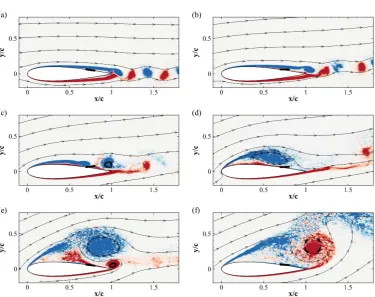
[image:14.595.82.474.49.506.2]Figure 9. Contour plot of the FTLEσT. Time increases from top to bottom, with a sampling time interval
of ∆t= 1.45c/U∞. The initial time (a-b) corresponds toα= 10o. The contour levels go from 0 (white) to 7U∞/c(red). The left and right columns are used for the baseline and controlled cases, respectively.
time interval [t0, t0+T]:
∆ = ∂x(t0+T,x0, t0)
∂x0
. (6)
[image:15.595.84.468.42.532.2]Figure 10. Spanwise pressure autocorrelation at various locations along the aerofoil suction side, computed at a distance of 0.1cfrom the wall. Time snapshots correspond to the ones given in Figure (2a). Solid line is the baseline case while symbols are for the case with flap.
a and b, the corresponding flow field is slightly asymmetric with two shear layers originating from the mid-chord region. The next two panels (b and c), show how the flow on the pressure side of the foil tends to reattach, while on the suction side an early separation is visible. Also, the shear layer at the trailing edge starts to roll up. As the shear layer roll-up process continues, a recirculation region is pro-gressively built up on the foil suction side (see panel e and f), ultimately leading to the formation of a large scale vortical structure, i.e., the dynamic stall vortex. As already remarked when analysing Figure (8), the sequence of panels a-c-e and b-d-f show again that the action of the flap retards the roll up of the shear layers. It is also highlighted that, while the large scale, dynamic stall vortex is formed, no vortices are shed from the trailing edge and an almost stable straight shear layer develops from it. The last two panels (i and j) show how the trailing edge shear layer rolls-up forming a fresh trailing edge vortex which pushes the dynamic stall vortex upwards causing its detachment. From panel j it also appears that the action of the flap strongly delays the formation of the trailing edge vortex.
Finally, we analyse the spanwise two-point pressure autocorrelation Rpp at
vari-ousxy coordinates. The autocorrelation is defined as
Rpp(z, r) =
p0(z)p0(z+r)
p02(z) , (7)
[image:16.595.85.455.48.338.2]the flow is mostly attached to the aerofoil, and all the points are in the laminar region. A wake induced, low amplitude pressure wave (amplitude ∼ 0.3% of the mean value) is visible at all the selected locations in panels a and b. In panel a, the controlled case shows the same behaviour except at the trailing edge, where the correlation reaches higher negative values. A more clear difference between the two cases is visible in panel b, that corresponds to the moment in which the angle of attack has reached 20o, and the separation point has moved upstream as shown in Figure (4a). In the baseline case the correlation rapidly goes to zero for all the points in the rear part of the aerofoil, indicating transition to turbulence. Differ-ently, the case with flap maintains higher values of the autocorrelation function in all the region covered by the flap motion. In later stages (panels c and d), when the trailing edge vortex is starting to roll up, the baseline case takes on a higher value of the correlation function (see Figure (8e)). The lower value in the controlled case is due to the action of the flap that delays the formation of the trailing edge vor-tex. Finally in panel e, most of the correlation values are quite low, except in the region spanned by the flap motion (in the controlled case), where the correlation seems to grow again because of the coherent local flow motion induced by the flap movement.
4. Conclusion
The present numerical study focuses on the use of a passive, self actuated, zero thickness flap as a control device able to limit the abrupt lift breakdown typical of dynamic stall. In particular, we have considered a NACA0020 aerofoil undergoing a ramp-up manoeuvre (i.e., incidence angleα initially increasing linearly from 0o to 20o with a reduced frequency of 0.12U∞/c, followed by a plateau atα= 20o) at a chord Reynolds number of 2×10⁴. After having conducted a detailed analysis of the baseline flow without flap, a number of different flap configurations have been considered having set as an aerodynamic objective one that:i)postpones the dynamic stall, ii) reduces the subsequent lift coefficient degradation rate and iii)
delivers a high efficiency throughout the whole manoeuvre. In particular, we have considered a family of rigid, membrane-like flaps hinged at the same location on the foil suction side (i.e., 70% of the chord) via a torsional spring. Each different flap configuration, obtained by modifying the flap natural frequency (i.e., spring stiffness) and its length, has been evaluated in terms of the aforementioned cri-teria. Finally, it has been found that a flap measuring 10% of the chord, with a natural frequency matching the shedding frequency of the baseline foil atα = 20o
time slowly reducing in intensity until the transient is completed and the steady angle of attack cyclic condition is recovered [21].
Acknowledgment
This research was partially funded by the EPSRC under grant EP/N020413 ”Quiet Aerofoil of the Next Generation”.
References
[1] R.L. Halfman, H.C. Johnson, and S.M. Haley, Evaluation of high-angle-of-attack aerodynamic-derivative data and stall-flutter prediction techniques, , DTIC Document, 1951.
[2] W.J. McCroskey,The phenomenon of dynamic stall., , DTIC Document, 1981.
[3] W.J. McCroskey,Unsteady airfoils, Annual review of fluid mechanics 14 (1982), pp. 285–311. [4] K. Mulleners, and M. Raffel,The onset of dynamic stall revisited, Experiments in fluids 52 (2012),
pp. 779–793.
[5] K. Mulleners, and M. Raffel,Dynamic stall development, Experiments in fluids 54 (2013), pp. 1–9. [6] C. Bruecker, and C. Weidner,Influence of self-adaptive hairy flaps on the stall delay of an airfoil in
ramp-up motion, Journal of Fluids and Structures 47 (2014), pp. 31–40.
[7] L.E. Ericsson, and J.P. Reding,Fluid dynamics of unsteady separated flow. Part I. Bodies of revolu-tion, Progress in Aerospace Sciences 23 (1986), pp. 1–84.
[8] L.E. Ericsson, and J.P. Reding,Fluid dynamics of unsteady separated flow. Part II. Lifting surfaces, Progress in Aerospace Sciences 24 (1987), pp. 249–356.
[9] L.E. Ericsson, and J.P. Reding,Fluid mechanics of dynamic stall part I. Unsteady flow concepts, Journal of fluids and structures 2 (1988), pp. 1–33.
[10] L.E. Ericsson, and J.P. Reding,Fluid mechanics of dynamic stall part II. Prediction of full scale characteristics, Journal of Fluids and Structures 2 (1988), pp. 113–143.
[11] T. Lee, and P. Gerontakos,Investigation of flow over an oscillating airfoil, Journal of Fluid Mechanics 512 (2004), pp. 313–341.
[12] C. Shih, L. Lourenco, L. Van Dommelen, and A. Krothapalli,Unsteady flow past an airfoil pitching at a constant rate, AIAA journal 30 (1992), pp. 1153–1161.
[13] N.L. Sankar, and W. Tang,Numerical solution of unsteady viscous flow past rotor sections, AIAA paper 85 (1985), p. 5.
[14] J.C. Wu,A study of unsteady turbulent flow past airfoils, Georgia Institute of Technology, 1988. [15] I.H. Tuncer, J.C. Wu, and C.M. Wang,Theoretical and numerical studies of oscillating airfoils, AIAA
journal 28 (1990), pp. 1615–1624.
[16] G.N. Barakos, and D. Drikakis,Computational study of unsteady turbulent flows around oscillating and ramping aerofoils, International journal for numerical methods in fluids 42 (2003), pp. 163–186. [17] S. Wang, D.B. Ingham, L. Ma, M. Pourkashanian, and Z. Tao,Numerical investigations on dynamic stall of low Reynolds number flow around oscillating airfoils, Computers & Fluids 39 (2010), pp. 1529–1541.
[18] E. Dumlupinar, and V.R. Murthy,Investigation of dynamic stall of airfoils and wings by CFD, in 29th AIAA Applied Aerodynamics ConferenceCurran, 2011, pp. 27–30.
[19] K. Gharali, and D.A. Johnson, Dynamic stall simulation of a pitching airfoil under unsteady freestream velocity, Journal of Fluids and Structures 42 (2013), pp. 228–244.
[20] J.A. Ekaterinaris, and M.F. Platzer,Computational prediction of airfoil dynamic stall, Progress in aerospace sciences 33 (1998), pp. 759–846.
[21] M.E. Rosti, M. Omidyeganeh, and A. Pinelli,Direct numerical simulation of the flow around an aerofoil in ramp-up motion, Physics of Fluids 28 (2016), 025106.
[22] T. Lee, and P. Gerontakos,Dynamic stall flow control via a trailing-edge flap, AIAA journal 44 (2006), pp. 469–480.
[23] B. Heine, K. Mulleners, G. Joubert, and M. Raffel,Dynamic stall control by passive disturbance generators, AIAA journal 51 (2013), pp. 2086–2097.
[24] D. Greenblatt, and I. Wygnanski,Dynamic stall control by periodic excitation, Part 1: NACA 0015 parametric study, Journal of Aircraft 38 (2001), pp. 430–438.
[25] D. Greenblatt, and I. Wygnanski,Effect of leading-edge curvature and slot geometry on dynamic stall control, AIAA Paper 3271 (2002), p. 2002.
[26] D. Bechert, M. Bruse, W. Hage, and R. Meyer, Fluid mechanics of biological surfaces and their technological application, Naturwissenschaften 87 (2000), pp. 157–171.
[27] G. Bramesfeld, and M.D. Maughmer,Experimental investigation of self-actuating, upper-surface, high-lift-enhancing effectors, Journal of aircraft 39 (2002), pp. 120–124.
[28] A.C. Carruthers, A.L.R. Thomas, and G.K. Taylor,Automatic aeroelastic devices in the wings of a steppe eagle Aquila nipalensis, Journal of Experimental Biology 210 (2007), pp. 4136–4149.
[29] M. Schatz, T. Knacke, F. Thiele, R. Meyer, W. Hage, and D.W. Bechert,Separation control by self-activated movable flaps, AIAA Paper 1243 (2004), p. 2004.
[30] J.U. Schluter,Lift enhancement at low Reynolds numbers using self-activated movable flaps, Journal of Aircraft 47 (2010), pp. 348–351.
V - Towards the control of the flow around aerofoils at high angle of attack using a self-activated deployable flap, Meccanica (under review).
[32] M.E. Rosti, M. Omidyeganeh, and A. Pinelli,Passive control of the flow around an aerofoil using a flexible, self adaptive flaplet, Journal of Fluid Mechanics (under review).
[33] M. Omidyeganeh, and U. Piomelli,Large-eddy simulation of three-dimensional dunes in a steady, unidirectional flow. Part 1. Turbulence statistics, Journal of Fluid Mechanics 721 (2013), pp. 454– 483.
[34] M. Omidyeganeh, and U. Piomelli,Large-eddy simulation of three-dimensional dunes in a steady, unidirectional flow. Part 2. Flow structures, Journal of Fluid Mechanics 734 (2013), pp. 509–534. [35] C.M. Rhie, and W.L. Chow,Numerical study of the turbulent flow past an airfoil with trailing edge
separation, AIAA journal 21 (1983), pp. 1525–1532.
[36] J. Kim, and P. Moin,Application of a fractional-step method to incompressible Navier-Stokes equa-tions, Journal of computational physics 59 (1985), pp. 308–323.
[37] S. Balay, S. Abhyankar, M. Adams, J. Brown, P. Brune, K. Buschelman, L. Dalcin, V. Eijkhout, W. Gropp, D. Kaushik, M. Knepley, L.C. McInnes, K. Rupp, B. Smith, S. Zampini, and H. Zhang, PETSc Web page; http://www.mcs.anl.gov/petsc.
[38] V.E. Henson, and U.M. Yang,BoomerAMG: a parallel algebraic multigrid solver and preconditioner, Applied Numerical Mathematics 41 (2002), pp. 155–177.
[39] J.L. Hess, and A.M.O. Smith, Calculation of potential flow about arbitrary bodies, Progress in Aerospace Sciences 8 (1967), pp. 1–138.
[40] J.G. Wong, A. Mohebbian, J. Kriegseis, and D.E. Rival,Rapid flow separation for transient inflow conditions versus accelerating bodies: An investigation into their equivalency, Journal of Fluids and Structures 40 (2013), pp. 257–268.
[41] A. Pinelli, I.Z. Naqavi, U. Piomelli, and J. Favier,Immersed-boundary methods for general finite-difference and finite-volume Navier–Stokes solvers, Journal of Computational Physics 229 (2010), pp. 9073–9091.
[42] J. Favier, A. Revell, and A. Pinelli,A Lattice Boltzmann–Immersed Boundary method to simulate the fluid interaction with moving and slender flexible objects, Journal of Computational Physics 261 (2014), pp. 145–161.
[43] J.C.R. Hunt, A.A. Wray, and P. Moin,Eddies, stream, and convergence zones in turbulent flows, Center for turbulence research report CTR-S88 (1988), pp. 193–208.
[44] G. Haller,Distinguished material surfaces and coherent structures in three-dimensional fluid flows, Physica D: Nonlinear Phenomena 149 (2001), pp. 248–277.