Abstract—Although extreme learning machine (ELM) has successfully been applied to a number of pattern recognition problems, only with the original ELM it can hardly yield high accuracy for the classification of hyperspectral images (HSIs) due to two main drawbacks. The first is due to the randomly generated initial weights and bias, which cannot guarantee the optimal output of ELM. The second is the lack of spatial information in the classifier as the conventional ELM only utilizes spectral information for classification of HSI. To tackle these two problems, a new framework for ELM based spectral-spatial classification of HSI is proposed, where probabilistic modelling with sparse representation and weighted composite features (WCF) are respectively employed to derive the optimized output weights and extract spatial features. First, the ELM is represented as a concave logarithmic likelihood function under statistical modelling using the maximum a posteriori (MAP) estimator. Second, the sparse representation is applied to the Laplacian prior to efficiently determine a logarithmic posterior with a unique maximum in order to solve the ill-posed problem of ELM. The variable splitting and the augmented Lagrangian are subsequently used to further reduce the computation complexity of the proposed algorithm and it has been proven a more efficient method for speed improvement. Third, the spatial information is extracted using the weighted composite features (WCFs) to construct the spectral-spatial classification framework. In addition, the lower bound of the proposed method is derived by a rigorous mathematical proof. Experimental
This work is supported in part by the National Nature Science Foundation of China (no. 61471132, 61372173, 61672008, 61572351), the Training program for outstanding young teachers of Guangdong Province (no. YQ2015057), Guangdong Provincial Application-oriented Technical Research and Development Special fund project (2016B010127006, 2017A050501039). Corresponding author: Dr. Zhijing Yang.
F. Cao, Z. Yang, and W.-K. Ling are with School of Information Engineering, Guangdong University of Technology, Guangzhou, China. ([email protected], [email protected], [email protected]).
J. Ren is with Department of Electronic and Electrical Engineering, University of Strathclyde, Glasgow, UK. ([email protected]).
H. Zhao is with School of Computer Science, Guangdong Polytechnic Normal University, Guangzhou, China ([email protected]).
M. Sun is with School of Computer Science and Technology, Tianjin University, Tianjin, China ([email protected]).
Jón Atli Benediktsson is with the Faculty of Electrical and Computer Engineering, University of Iceland, Reykjavik, Iceland ([email protected]).
results on three publicly available HSI data sets demonstrate that the proposed methodology outperforms ELM and also a number of state-of-the-art approaches.
Index Terms—hyperspectral image (HSI), spectral-spatial classification, extreme learning machine (ELM), maximum a posterior (MAP), sparse representation, Laplacian prior.
I. INTRODUCTION
ith rich spectral and spatial information contained in a three-dimensional hypercube, hyperspectral images (HSI) provide a unique way for characterizing objects in geographical scenes, especially remote sensing images [1]. However, classification of high dimensional data such as HSI is still challenging, particularly due to the unfavorable ratio between the limited number of training samples and large number of spectral bands, i.e., the Hughes phenomenon [2]-[4]. To tackle this problem, a number of feature extraction and data classification approaches have been proposed [12]. These include the singular spectrum analysis (SSA) [5]-[8], segmented auto-encoders [11], principal component analysis (PCA) and its variations [13], [14], and support vector machines (SVM) [9]. In addition, a locality adaptive discriminant analysis (LADA) approach has been proposed for spectral-spatial classification of hyperspectral images [10]. In [15], a multitask joint sparse representation and stepwise MRF optimization (MSMRF) method is proposed for HSI classification. In [16], the manifold ranking (MR) is applied for salient band selection of HSI. Although these approaches have produced good results in term of classification accuracy, their performance can be further improved by addressing two main difficulties: (1) Inaccurate classification with a large number of spectral bands yet limited training samples, and (2) relatively low efficiency for processing high dimensional HSI data.
As a single forward layer neural network, the extreme learning machine (ELM) is a fast and effective machine learning method and has received a wide attention due to its good performance [17]-[19]. The ELM does not tune the hidden layer parameters once the number of hidden layer nodes has been determined. In ELM, the weight and bias vectors between the input layer and the hidden layer are initially randomly generated, which are independent of the training samples and the specific applications [1]. ELM has achieved good performance in many applications [20]-[23], even for HSI classifications [24]-[28]. In [24] and [25], bilateral filtering and
Sparse Representation Based Augmented Multinomial
Logistic Extreme Learning Machine with Weighted
Composite Features for Spectral-Spatial Classification
of Hyperspectral Images
Faxian Cao,
Student Member, IEEE,
Zhijing Yang,
Member, IEEE,
Jinchang Ren,
Senior Member, IEEE
,Wing-Kuen Ling,
Senior Member, IEEE,
Huimin Zhao, Meijun Sun, Jón Atli Benediktsson,
Fellow, IEEE
extended morphological profiles were used for feature extraction, followed by ELM for classification. In [26]-[28], ELM was employed for classification with feature extracted using local binary pattern (LBP) and Gabor filters. Although these ELM-based methods have achieved good performance to some extent, they ignore one very important issue of ELM that the randomly generated input weights and bias of ELM may cause ill-posed problems. Based on this perspective, we first propose an improved ELM, namely the Augmented Sparse Multinomial Logistic ELM (ASMLELM) for HSI classification. Based on the proposed ASMLELM, we additionally present weighted composite features (WCFs) for extracting the spatial information. To this end, we finally propose ASMLELM-WCFs as a novel framework for spectral-spatial classification of HSI.
The main contributions of this paper can be highlighted as follows. First, we propose the augmented spare multinomial logistic extreme learning machine (ASMLELM) to alleviate the ill-posed problem of ELM, which is caused by the randomly generated weights and bias. In ASMLELM, the ELM is represented by a maximum a posteriori (MAP) based probabilistic model, which is further represented by a concave logarithmic likelihood function (LLF). To improve the sparsity of the learnt weights and guarantee the logarithmic posterior to have a unique maximum, the sparse representation, i.e. the Laplacian prior/regularized term, is employed for representing the ELM [29]-[32]. As such, optimal weight and bias are determined for the ELM, followed by variable splitting and augmented Lagrangian [33] to further improve the efficiency. Second, by combining the composite kernels (CK) [34] and weighted mean filters (WMFs) [35], the weighted composite features (WCFs) are used to extract spatial features and further improve the classification accuracy. Accordingly, three improved spectral-spatial classifiers are derived, which include the ELM, the nonlinear ELM (NLELM) and the kernel ELM (KELM) based classifiers, i.e., ASMLBELM-WCFs, ASMLNLELM-WCFs, and ASMLKELM-WCFs.
Third, inspired by the sparse multinomial logistic regression (SMLR) [29], [36], [37], the generalization bounds of the proposed method are derived, which can provide a theoretical insight of and further justification for our proposed methods. The rest of this paper is organized as follows. In Section II, the background of the ELM is introduced. The proposed method is detailed in Section III. Section IV reports the experimental results in benchmarking with a few state-of-the-art approaches. Finally, some conclusions are drawn in Section V.
II.THE EXTREME LEARNING MACHINE (ELM) A. Basic Concepts of ELM
The ELM is a generalized single layer feedforward neural network (SLFNs) [1], [17]. The weight vector and the bias between the input layer and hidden layer are randomly initialized. Once the initial values for the weight/bias vectors are assigned, the hidden layer output matrix remains unchanged in the learning process [1].
Let 𝑋 ≡ (𝑥1, 𝑥2, … , 𝑥𝑁) ∈ 𝑅𝑑×𝑁 be the training data of a HSI, which has N pixels and each pixel has a d-dimensional feature. Let 𝑌 = (𝑦1, 𝑦2, … , 𝑦𝑁) ∈ 𝑅𝑀×𝑁 be a matrix representing the class label of the training samples, where M is the number of classes in the datasets. Given a pixel label 𝑦𝑖, if it belongs to the k-th class, we have
𝑦𝑖,𝑗= { 0, 𝑜𝑡ℎ𝑒𝑟𝑤𝑖𝑠𝑒.1, 𝑗 = 𝑘,
The model of a single hidden layer neural network with L hidden neurons and the activation function 𝐻(𝑥) can be expressed as follows:
∑𝐿𝑗=1𝛽𝑗𝐻(𝑤𝑗𝑇𝑥𝑖+ 𝑏𝑗) = 𝑦𝑖, i=1,2,…,N (1) where 𝛽𝑗 represents the weight vector between the hidden layer and the output layer; 𝑤𝑗 and 𝑏𝑗 are the weight vector and bias from the inputs to the hidden layer, respectively; 𝐻(𝑤𝑗𝑇𝑥𝑖+ 𝑏𝑗) represents the output of the j-th hidden neuron with respect to the input sample 𝑥𝑖. Obviously, (1) can be further expressed in the following matrix form:
𝐻𝑇𝛽 = 𝑌𝑇 (2) where 𝛽 = [𝛽1 ⋯ 𝛽𝑀]𝐿×𝑀, 𝐻 =[𝐻(𝑥1) ⋯ 𝐻(𝑥𝑛)]𝐿×𝑁, and 𝐻(𝑥𝑖) = [𝐻1(𝑥𝑖) ⋯ 𝐻𝐿(𝑥𝑖)]𝐿×1𝑇 . H is the hidden layer output matrix, and 𝛽 is the output weight matrix between the hidden layer and the output layer.
From (2), 𝛽 can be simply obtained below, where † is the Moore Penrose generalized inverse of a matrix [17].
𝛽 = (𝐻𝑇)†𝑌𝑇 (3) B. Constrained Optimization of the ELM
The constrained optimization of the ELM aims to achieve not only the smallest training error but also the smallest output weights [19]:
min ∥ 𝐻𝑇𝛽 − 𝑌𝑇∥2 and ∥ 𝛽 ∥2. (4) According to the Bartlett’s neural network generalization theory [38], the smaller weights will result in a smaller training error of the feedforward neural networks. As a result, (4) can be rewritten as:
min
𝛽,𝜉𝑖 𝐿𝐸𝐿𝑀= 1 2∥ 𝛽 ∥𝐹
2+ 𝐶1
2∑ ∥ 𝜉𝑖∥2
2 𝑁
𝑖=1 ,
s. t. 𝐻𝑇(𝑥𝑖)𝛽 = 𝑦i𝑇− 𝜉𝑖𝑇, i=1,..,N (5) where 𝜉𝑖 is the training error for the training sample 𝑥𝑖, C is the regularization parameter.
Based on the Karush-Kuhn-Tucker (KKT) theorem [39], training the ELM is equivalent to solve the following dual optimization problem:
min
(𝛽,𝛼,𝜉𝑖)𝐿𝐸𝐿𝑀= 1 2∥ 𝛽 ∥𝐹
2+ 𝐶1
2∑ ∥ 𝜉𝑖∥2
2 𝑁
𝑖=1 − ∑𝑁𝑖=1∑𝑀𝑗=1𝛼𝑖,𝑗(𝐻𝑇(𝑥𝑖)𝛽𝑗− 𝑦𝑖,𝑗+ 𝜉𝑖,𝑗) (6) where 𝛽𝑗 is the column vector of the matrix 𝛽, and 𝛼𝑖,𝑗 is the Lagrange multiplier.
From the KKT theorem, we can further derive 𝜕𝐿𝐸𝐿𝑀
𝜕𝛽𝑗 = 0 → 𝛽 = 𝐻 ∗ 𝛼, (7) 𝜕𝐿𝐸𝐿𝑀
𝜕𝜀𝑖 = 0 → 𝛼𝑖= 𝐶𝜀𝑖, 𝑖 = 1, … , 𝑁, (8) 𝜕𝐿𝐸𝐿𝑀
𝜕𝛼𝑖 = 0 → 𝐻 𝑇(𝑥
Then, it can be shown that the output weight 𝛽 is:
𝛽 = 𝐻 (𝐶𝐼+ 𝐻𝑇𝐻)−1𝑌𝑇. (10) The activation functions of the neurons in the hidden layer are unknown, and any kernel satisfying the Mercer’s conditions can be used:
{ 𝛀𝐾𝐸𝐿𝑀= 𝐻
𝑇∗ 𝐻,
Ω𝐾𝐸𝐿𝑀(𝑥𝑖, 𝑥𝑗): h(𝑥𝑖)𝑇h(𝑥𝑖) = 𝐾(𝑥𝑖, 𝑥𝑗). (11) In fact, the Gaussian kernel is one of the good choices
𝐾𝐸𝐿𝑀(𝑥𝑖, 𝑥𝑗) = exp (− ∥𝑥𝑖−𝑥𝑗∥2
2∗𝜎𝐸𝐿𝑀2 ) (12) Based on the above analysis, two well-known constrained optimization methods of ELM have been proposed [19]. One is to define 𝛽 in (10) without a kernel, namely nonlinear ELM (NLELM), and the other is to use the kernel function to form the kernel ELM (KELM) as given below:
𝛽𝑁𝐿𝐸𝐿𝑀 = 𝐻(𝐶𝐼+ 𝐻𝑇𝐻)−1𝑌𝑇, (13) 𝛽𝐾𝐸𝐿𝑀 = (𝐶𝐼+ 𝐾(𝑥𝑖, 𝑥𝑗))−1𝑌𝑇. (14)
III.THE PROPOSED ASMLELMFRAMEWORK
A. Sparse Multinomial Logistic Extreme Learning Machine (SMLELM)
The goal of a supervised learning algorithm is to design a classifier based on a set of N training samples that is capable of distinguishing M classes on the basis of an input vector of length d [29]. Under the multinomial logistic regression model [40], 𝛽 in (3), (13) and (14) can be transformed to a new form via a probability model. If the training sample 𝑥𝑖 belongs to the k-th class, the probability model can be represented by the following equation:
𝑃(𝑦𝑖,𝑘= 1|𝐻(𝑥𝑖), 𝛽) = 𝑒𝑥𝑝 (𝛽𝑘
𝑇𝐻(𝑥
𝑖))
∑𝑀𝑗=1𝑒𝑥𝑝 (𝛽𝑗𝑇𝐻(𝑥𝑖)). (15) In (3), (13), (14) and (15), 𝛽 may not be optimal due to the ill-posed problem of ELM. Therefore, it is important to find the optimal 𝛽 to obtain high classification accuracy, where 𝛽 can be estimated again after presenting the ELM by a probabilistic model. To this end, the maximum likelihood (ML) estimation is introduced to the ELM. Let 𝛽 = [𝛽1; 𝛽2; ⋯ ; 𝛽𝑀](𝐿∗𝑀)×1 be a column vector with 𝐿 × 𝑀 elements, a simple maximization of the logarithmic likelihood is given as follows:
𝑚𝑎𝑥
𝛽 𝐿(𝛽) = ∑ (∑ 𝑦𝑖,𝑗𝛽𝑗
𝑇𝐻(𝑥
𝑖) 𝑀
𝑗=1 𝑁
𝑖=1 −
𝑙𝑜𝑔 ∑𝑀𝑗=1𝑒𝑥𝑝 (𝛽𝑗𝑇𝐻(𝑥𝑖))). (16) In order to maximize L(𝛽), consider the second order Taylor series of L(𝛽) evaluated at 𝛽′:
𝐿(𝛽) − 𝐿(𝛽′) = (𝛽 − 𝛽′)𝑇𝛻𝐿(𝛽′) + 1
2(𝛽 − 𝛽
′)𝑇𝛻2𝐿(𝛽′+ 𝜌(𝛽 − 𝛽′))(𝛽 − 𝛽′), ≥ (𝛽 − 𝛽′)𝑇𝛻𝐿(𝛽′) +1
2(𝛽 − 𝛽
′)𝑇𝐵(𝛽 − 𝛽′) (17) where 𝜌 ∈ (0,1) and
𝐵 ≡ −12[𝑰 −𝟏𝟏𝑀𝑻] ⊗ 𝐻𝐻𝑇 (18) where 𝑰 ∈ 𝑅𝑀×𝑀 is an identity matrix, 𝟏 = [1, 1, … ,1]𝑇 and ⊗ is the Kronecker matrix product [40], [41]. Then, the ML estimation can be expressed as follows:
𝛽̂ = 𝑎𝑟𝑔 𝑚𝑎𝑥
𝛽 {𝛽
𝑇( 𝛻𝐿(𝛽′) − 𝐵𝛽′) +1 2𝛽
𝑇𝐵𝛽}. (19) Note that the dimensions of 𝐻 and 𝐻𝐻𝑇 are 𝐿 × 𝑁 and 𝐿 × 𝐿, where 𝐿 and 𝑁 refer respectively to the number of hidden neuron of ELM and the number of training samples. The dimension of 𝐵 is 𝑀𝐿 × 𝑀𝐿, where 𝑀 is the number of classes. For 𝛽 and 𝛽′in (19), their dimensions are 𝑀𝐿×1.
Hence, 𝛽 at the (t+1)-th iteration can be expressed by a simple updating equation:
𝛽̂𝑡+1= 𝐵−1(𝐵𝛽̂𝑡− 𝛻𝐿(𝛽̂𝑡)). (20) Eq. (20) is very similar to an iteratively reweighted least squares (IRLS) algorithm [42]. However, the Hessian matrix in the IRLS algorithm is replaced by matrix B. Since 𝐵−1 can be precomputed, it is a big advantage of the proposed approach. Compared to the IRLS algorithm, whose Hessian matrix must be inverted at each iteration [29], [43], our proposed approach is much more efficient.
However, the concave LLF value can be arbitrarily large if the training data is separable. From [29], it is known that a prior on the logarithmic likelihood is crucial. In order to address the ill-posed problem in ELM, the prior/regularized term is adopted on 𝛽. Here, the Laplacian prior is used:
𝐿1(𝛽) = 𝐿(𝛽) − 𝐿(𝛽′) + 𝑙𝑜𝑔𝑝(𝛽) (21) 𝑝(𝛽) ∝ 𝑒𝑥𝑝 (−𝜆 ∥ 𝛽 ∥1) (22) and ∥ 𝛽 ∥1=∑ |𝛽𝑙 𝑙| denotes the l1 norm and |𝛽𝑙|=√𝛽𝑙2.
Consider the following inequality for h>0 and u>0: ℎ + 𝑢 ≥ 2√ℎ√𝑢𝑦𝑖𝑒𝑙𝑑𝑠→ √𝑢 ≤12(𝑢
√ℎ+ √ℎ). (23) For any 𝛽′, we have
−𝜆 ∥ 𝛽 ∥1≥ −12𝜆(∑ 𝛽𝑙 2
|𝛽𝑙′|+ ∑ |𝛽𝑙 𝑙′|
𝑙 ). (24) Therefore, the following term can be maximized:
𝑚𝑎𝑥
𝛽 { 𝛽
𝑇(∇𝐿
1(𝛽′) − 𝐵𝛽′) +12𝛽𝑇(𝐵 − 𝜆)𝛽}, (25) ⋀ = 𝑑𝑖𝑎𝑔{|𝛽11|−1, … , |𝛽𝐿𝑀|−1}. (26) Finally, (20) can be expressed by the following equation:
𝛽̂𝑡+1= (𝐵 − 𝜆⋀𝑡)−1(𝐵𝛽̂𝑡− ∇𝐿(𝛽̂𝑡)). (27) From the above, it can be seen that the Laplacian prior/regularized term is applied to 𝛽 with 𝜆 acting as a regularization parameter. The Laplacian prior imposed on the sparse multinomial logistic ELM (SMLELM) controls the complexity of the SMLELM classifier and improves the generalization capacity of the SMLELM, where 𝑝(𝛽) in (22) forces most components of 𝛽 to become zero.
B. Augmented Sparse Multinomial Logistic Extreme Learning Machine (ASMLELM)
reduce the complexity of the proposed SMLELM, which has transformed the proposed SMLELM into a new form namely augmented SMLELM (ASMLELM) as detailed below.
Variable splitting is straightforward approach which consists a procedure to create new variables [50], where the problem defined in (21) is equivalent to:
(𝛽̂, 𝑣̂) = 𝑎𝑟𝑔 min
𝛽,𝑣{−L(𝛽) + 𝜆 ∥ 𝑣 ∥1} s.t. 𝛽 = 𝑣. (28) The aforementioned optimization problem can be solved via applying the direction method of multipliers [51] (see also [52] and the references therein). So we call this neural network as the augmented SMLELM (ASMLELM). Applying the augmented Lagrangian [50] to (28), the solution of (28) at the (t+1)-th iteration can be rewritten as follows:
𝛽̂𝑡+1= 𝑎𝑟𝑔 min
𝛽 {−L(𝛽) + 𝛾
2∥ 𝛽 − 𝑣
𝑡− 𝑏𝑡∥2}, (29) 𝑣̂𝑡+1= 𝑎𝑟𝑔 min
𝑣 { 𝜆 ∥ 𝑣 ∥1+ 𝛾
2∥ 𝛽
𝑡+1− 𝑣 − 𝑏𝑡∥2}, (30)
𝑏𝑡+1 = 𝑏𝑡− 𝛽𝑡+1+ 𝑣𝑡+1 (31) where 𝛾 ≥ 0 is the weight of the augmented SMLELM (ASMLELM). For any 𝛾 ≥ 0, the sequence 𝛽̂𝑡 converges to a minimizer [45], [48] [50]. For easy implementation and tuning the parameters, we set 𝛾 = 10𝜆 in our experiments. The solution of the problem defined in (28) is the simple soft-threshold rule [51], [45], which can be expressed as:
𝑣𝑡+1= max {0, 𝑎𝑏𝑠(𝑒) − 𝜆/𝛾}, (32) 𝑒 = 𝛽𝑡+1− 𝑏𝑡. (33) When the same ASMLELM framework is applied respectively to the BELM, NLELM and KELM, three new spectral algorithms for performing the HSI classification can be generated, which are named as ASMLBELM for the basic ELM, ASMLNLELM for NLELM and ASMLKELM for KELM. The pseudocodes for these three methods are shown in Algorithm 1.
Algorithm 1:The ASMLELM for the basic ELM, the NLELM and the KELM
Input: The training sample pairs {𝑋𝑡𝑟𝑎𝑖𝑛 = (𝑥1, 𝑥2, … , 𝑥N) and 𝑌𝑡𝑟𝑎𝑖𝑛= (𝑦1, 𝑦2, … , 𝑦𝑁)}, where N is the number if training samples. As well as the parameters 𝜆, b = 0.
Training phase:
L: The number of nodes in a hidden layer. 𝐻(): The sigmoid function.
𝛽: The output weight in the hidden layer.
1: Randomly generate input weights {𝑤1, … 𝑤𝐿} and bias {𝑏1, … , 𝑏𝐿} to obtain the preliminary value of 𝛽. 2: For each training sample 𝒙𝐢, calculate the hidden layer matrix
H(𝑥𝑖) = [𝐻1(𝑤1∗ 𝒙𝒊+ 𝑏1), . . . , 𝐻𝐿(𝑤𝐿∗ 𝒙𝒊+ 𝑏𝐿)]𝐿×1𝑇 . 3: Calculate the preliminary output weight for 𝛽
(1) 𝛽 = (𝐻𝑇)†𝑌𝑇 for the ASMLBELM. (2) min
𝛽,𝜉𝑖 𝐿𝐸𝐿𝑀= 1 2∥ 𝛽 ∥𝐹
2+ 𝐶1
2∑ ∥ 𝜉𝑖∥2
2 𝑁
𝑖=1 , s. t. 𝐻𝑇(𝑥𝑖)𝛽 = 𝑦i𝑇− 𝜉𝑖𝑇, i=1,..,N. Here, 𝛽 = 𝐻 ∗ (𝐶𝐼+ 𝐻𝑇𝐻)−1𝑌𝑇 for the ASMLNLELM.
(3) Let π = (𝐼
𝐶+ 𝐻
𝑇𝐻)−1𝑌𝑇 and the Gaussian kernel 𝐾
𝑇rain(𝑥𝑖, 𝑥𝑗) = exp (− ∥𝑥𝑖−𝑥𝑗∥2
2∗𝜎𝐸𝐿𝑀2 ). Then, π = (𝐼
𝐶+ 𝐾𝑇𝑟𝑎𝑖𝑛)
−1𝑌𝑇 for the ASMLKELM. 4. Represent the ELM by a probability model (1) 𝑃(𝑦𝑖,𝑘= 1|𝐻(𝑥𝑖), 𝛽) = 𝑒𝑥𝑝 (𝛽𝑘
𝑇𝐻(𝑥
𝑖))
∑𝑀𝑗=1𝑒𝑥𝑝 (𝛽𝑗𝑇𝐻(𝑥𝑖)) for the ASMLBELM and the ASMLNLELM. (2) 𝑃(𝑦𝑖,𝑘= 1|𝐾𝑡𝑟𝑎𝑖𝑛(𝑥𝑖), π) = 𝑒𝑥𝑝 (π𝑘
𝑇𝐾 𝑇rain)
∑𝑀𝑗=1𝑒𝑥𝑝 (π𝑗𝑇𝐾𝑇rain) for the ASMLKELM.
5. ASMLELM: The ML estimate based on the sparse representation with the Laplacian prior via variable splitting and constrained optimization.
5.1 𝛽̂ = 𝑎𝑟𝑔 max
𝛽 𝛽
𝑇( ∇𝐿(𝛽′) − 𝐵𝛽′) +1 2𝛽
𝑇(𝐵 − 𝜆⋀𝑡)𝛽. 5.2 Set t=0.
5.3 𝛽̂𝑡+1 = arg min
𝛽 −L(𝛽) + 10𝜆
2 ∥ 𝛽 − 𝑣
𝑡− 𝑏𝑡∥2. 5.4 𝑣̂𝑡+1= arg arg min
𝑣 𝜆 ∥ 𝑣 ∥1+ 10𝜆
2 ∥ 𝛽
𝑡+1− 𝑣 − 𝑏𝑡∥2. 5.5 𝑏𝑡+1 = 𝑏𝑡− 𝛽𝑡+1+ 𝑣𝑡+1.
5.6 Increase t to t+1; If the ASMLKELM is applied, replace 𝛽 by π.
5.7 Quit the algorithm if the stopping criterion is met; otherwise, go back to Step 5.3.
Prediction phase: Input: 𝑋𝑡𝑒𝑠𝑡≡ (𝑥1, 𝑥2, … , 𝑥n) 1: (1) Calculate the output layer matrix
H∗(𝒙𝒊) = [𝐻1(𝑤1𝒙𝒊+ 𝑏1), … , 𝐻𝐿(𝑤𝐿𝒙𝒊+ 𝑏𝐿)]𝐿×1𝑇 i=1,…,N for ASMLBELM and ASMLNLELM. (2) 𝐾𝑡𝑒𝑠𝑡= H∗𝑇H = exp (−
∥𝑥𝑖−𝑥𝑗∥2
2: (1) 𝑃(𝑦𝑖,𝑘|𝐻∗(𝑥𝑖), 𝛽) = 𝑒𝑥𝑝 (𝛽𝑘 𝑇H∗(𝒙𝒊))
∑𝑀𝑗=1𝑒𝑥𝑝 (𝛽𝑗𝑇H∗(𝒙𝒊)) for ASMLBELM and AMSLNLELM. (2) 𝑃(𝑦𝑖,𝑘|𝐾𝑡𝑒𝑠𝑡, π) = 𝑒𝑥𝑝 (π𝑘
𝑇𝐾 𝑡𝑒𝑠𝑡(𝑥𝑖))
∑𝑀𝑗=1𝑒𝑥𝑝 (π𝑗𝑇𝐾𝑡𝑒𝑠𝑡) for the ASMLKELM.
Algorithm 2: ASMLELM with WCFs (ASMLBELM-WCFs, ASMLNLELM-WCFs, ASMLKELM-WCFs) Input: The training spectral feature 𝑥𝑡𝑟𝑎𝑖𝑛𝑤 = (𝑥1𝑤, 𝑥2𝑤, … , 𝑥N𝑤), the spatial feature 𝑥𝑡𝑟𝑎𝑖𝑛𝑠 ≡ (𝑥1𝑠, 𝑥2𝑠, … , 𝑥N𝑠), and the labelled data 𝑌𝑡𝑟𝑎𝑖𝑛= (𝑦1, 𝑦2, … , 𝑦𝑁), as well as the parameters C, 𝜆, b = 0.
Training phase:
L: The number of nodes in a hidden layer. 𝐻(): The sigmoid function.
The output weight of the hidden layer 𝛽.
1: Randomly generate input weight {𝑤1, … 𝑤𝐿} and bias {𝑏1, … , 𝑏𝐿} to obtain the preliminary value of 𝛽. 2: For any training sample 𝒙𝐢, calculate the hidden layer matrix
𝐻𝑤(𝑥i𝑤) = [𝐻1(𝑤1∗ 𝑥i𝑤+ 𝑏1), . . . , 𝐻𝐿(𝑤𝐿∗ 𝑥i𝑤+ 𝑏𝐿)]𝐿×1𝑇 and 𝐻𝑠(𝑥i𝑠) = [𝐻1(𝑤1∗ 𝑥i𝑠+ 𝑏1), . . . , 𝐻𝐿(𝑤𝐿∗ 𝑥i𝑠+ 𝑏𝐿)]𝐿×1𝑇 , where (1) 𝐻 = μ𝐻𝑤+ (1 − μ)𝐻𝑠 for the ASMLBELM-WCFs.
(2) 𝐻 = √μ𝐻𝑤+ √(1 − μ)𝐻𝑠 for the ASMLNLELM-WCFs and the ASMLKELM-WCFs. 3: Calculate the preliminary output weight for 𝛽
(1) 𝛽 = (𝐻𝑇)†𝑌𝑇 for the ASMLBELM-WCFs. (2) min
𝛽,𝜉𝑖 𝐿𝐸𝐿𝑀= 1 2∥ 𝛽 ∥𝐹
2+ 𝐶1
2∑ ∥ 𝜉𝑖∥2
2 𝑁
𝑖=1 , s. t. 𝐻𝑇(𝑥𝑖)𝛽 = 𝑦i𝑇− 𝜉𝑖𝑇 i=1,..,N. Here, 𝛽 = 𝐻 ∗ (𝐶𝐼+ 𝐻𝑇𝐻)−1𝑌𝑇 for the ASMLNLELM-WCFs.
(3) π = (𝐼
𝐶+ 𝐾𝑡𝑟𝑎𝑖𝑛) −1𝑌𝑇, 𝐾
𝑡𝑟𝑎𝑖𝑛 = μ𝐻𝑤𝑇𝐻𝑤+ (1 − μ)𝐻𝑠𝑇𝐻𝑠 = μ𝐾𝐻𝑤+ (1 − μ)𝐾𝐻𝑠 for ASMLKELM-WCFs.
4.Represent the ELM by a probability model 𝑃(𝑦𝑖,𝑘= 1|𝐻(𝑥𝑖), 𝛽) = 𝑒𝑥𝑝 (𝛽𝑘
𝑇𝐻(𝑥
𝑖))
∑𝑀𝑗=1𝑒𝑥𝑝 (𝛽𝑗𝑇𝐻(𝑥𝑖)) for the ASMLBELM-WCFs and the ASMLNLELM-WCFs.
𝑃(𝑦𝑖,𝑘= 1|𝐾𝑡𝑟𝑎𝑖𝑛(𝑥𝑖), π) = 𝑒𝑥𝑝 (π𝑘
𝑇𝐶𝐾
𝑡𝑟𝑎𝑖𝑛(𝑥𝑖))
∑𝑀𝑗=1𝑒𝑥𝑝 (π𝑗𝑇𝐾𝑡𝑟𝑎𝑖𝑛(𝑥𝑖)) for the ASMLKELM-WCFs.
5. ASMLELM : The ML estimate based on the sparse representation with the Laplacian prior via variable splitting and constrained optimization.
5.1 𝛽̂ = 𝑎𝑟𝑔 max
𝛽 {𝛽
𝑇( ∇𝐿(𝛽′) − 𝐵𝛽′) +1 2𝛽
𝑇(𝐵 − 𝜆)𝛽}. 5.2 Set t=0.
5.3 𝛽̂𝑡+1= arg min
𝛽 {−L(𝛽) + 10𝜆
2 ∥ 𝛽 − 𝑣
𝑡− 𝑏𝑡∥2}. 5.4 𝑣̂𝑡+1= arg arg min
𝑣 { 𝜆 ∥ 𝑣 ∥1+ 10𝜆
2 ∥ 𝛽
𝑡+1− 𝑣 − 𝑏𝑡∥2}. 5.5 𝑏𝑡+1 = 𝑏𝑡− 𝛽𝑡+1+ 𝑣𝑡+1.
5.6 Increase t to t+1; If the ASMLKELM-WCFs is applied, replace 𝛽 by π.
5.7 Quit the algorithm if the stopping criterion is met; otherwise, go back to Step 5.3.
Prediction phase:
Input: The testing spectral feature 𝑥𝑡𝑒𝑠𝑡𝑤 = (𝑥1𝑤, 𝑥2𝑤, … , 𝑥n𝑤), and the spatial feature 𝑥𝑡𝑒𝑠𝑡𝑠 ≡ (𝑥1𝑠, 𝑥2𝑠, … , 𝑥n𝑠). 1: Calculate the output layer matrix
𝐻𝑤∗(𝑥i𝑤) = [𝐻1(𝑤1∗ 𝑥i𝑤+ 𝑏1), . . . , 𝐻𝐿(𝑤𝐿∗ 𝑥i𝑤+ 𝑏𝐿)]𝐿×1𝑇 , and 𝐻𝑠∗(𝑥i𝑠) = [𝐻1(𝑤1∗ 𝑥i𝑠+ 𝑏1), . . . , 𝐻𝐿(𝑤𝐿∗ 𝑥i𝑠+ 𝑏𝐿)]𝐿×1𝑇 , where (1) 𝐻∗= μ𝐻𝑤∗ + (1 − μ)𝐻𝑠∗ for the ASMLBELM-WCFs. (2) 𝐻∗= √μ𝐻𝑤∗ + √(1 − μ)𝐻𝑠∗ for the ASMLNLELM-WCFs.
(3) 𝐻∗= √μ𝐻𝑤∗ + √(1 − μ)𝐻𝑠∗, 𝐾𝑡𝑒𝑠𝑡= μ𝐻𝑤∗𝑇𝐻𝑤∗ + (1 − μ)𝐻𝑠∗𝑇𝐻𝑠∗= μ𝐾𝐻𝑤+ (1 − μ)𝐾𝐻𝑠 for ASMLKELM-WCFs.
2: (1) 𝑃(𝑦𝑖,𝑘|𝐻∗(𝑥𝑖), 𝛽) = 𝑒𝑥𝑝 (𝛽𝑘 𝑇H∗(𝒙𝒊))
∑𝑀𝑗=1𝑒𝑥𝑝 (𝛽𝑗𝑇H∗(𝒙𝒊)) for the ASMLBELM-WCFs and the ASMLNLELM-WCFs.
(2) 𝑃(𝑦𝑖,𝑘|𝐾𝑡𝑒𝑠𝑡(xi), 𝛽) = 𝑒𝑥𝑝 (𝜋𝑘 𝑇𝐾𝑡𝑒𝑠𝑡(𝑥
𝑖)) ∑𝑀 𝑒𝑥𝑝 (
C. Weighted Composite Features Based ASMLELM (ASMLELM-WCFs)
Until now in our discussion, the ASMLELM has only used the spectral information of the HSI data for classification. Since a pixel and its spatial neighboring pixels very likely belong to the same class [1], the spatial information is also essential for data classification in HSI. To this end, the WCFs are used to perform the spectral spatial classification for the proposed ASMLELM framework and form the new approach namely ASMLELM-WCFs.
For a given pixel 𝑥𝑖, let its spatial coordinates be (p, q), the local pixel neighborhood centered at 𝑥𝑖 is 𝑁𝑏(𝑥𝑖) = {𝑥 = (𝑝, 𝑞)|𝑝 ∈ [𝑝 − 𝑎, 𝑝 + 𝑎]; 𝑞 ∈ [𝑞 − 𝑎; 𝑞 + 𝑎]} , a=(wopt-1)/2 where wopt is the width/height of the neighborhood window. Let 𝑥𝑖𝑤 be the spectral feature of the sample 𝑥𝑖and 𝑥𝑖𝑠 be the information extracted from a local spatial neighborhood of 𝑥𝑖. Let {𝑥𝑖, 𝑥𝑖1, 𝑥𝑖2, … , 𝑥𝑖𝑠} be the pixels in 𝑁𝑏(𝑥𝑖), where s = wopt2− 1. Then 𝑥
𝑖𝑠can be represented as 𝑥𝑖𝑠= ∑ 𝑥𝑐𝑣𝑐
𝑥𝑐∈𝑁𝑏(𝑥𝑖)
∑ 𝑣𝑐=𝑥𝑖+ ∑ 𝑣𝑐𝑥𝑖𝑐 𝑠 𝑐=1 1 + ∑𝑠𝑐=1𝑣𝑐 𝑥𝑐∈𝑁𝑏(𝑥𝑖)
⁄
where the weight 𝑣𝑐= exp {−𝑧 ∥ 𝑥𝑖− 𝑥𝑖𝑐∥2} measuring the spectral distance between the central pixel, 𝑥𝑖, and the neighboring pixels, 𝑥𝑖𝑐 (𝑥𝑖𝑐∈ 𝑁𝑏(𝑥𝑖)). Following the setting in [35], we set 𝑧 = 0.2 in this work.
The output matrix of the hidden layer defined in (2) and (13) can be expressed as:
𝐻 = μ𝐻𝑤+ (1 − μ)𝐻𝑠, (34) 𝐻𝑤= [𝐻𝑤(𝑥1𝑤) ⋯ 𝐻𝑤(𝑥n𝑤)]𝐿×𝑁, (35) 𝐻𝑠= [𝐻𝑠(𝑥1𝑠) ⋯ 𝐻𝑠(𝑥n𝑠)]𝐿×𝑁 (36) and μ is a coefficient balancing the spectral and spatial information.
For the KELM defined in (14), 𝛽 can be defined as follows: 𝛽 = (𝐶𝐼 + K)−1𝑌𝑇, (37) K = μ𝐾𝐻𝑤+ (1 − μ)𝐾𝐻𝑠, (38) 𝐾𝐻𝑤(𝑥𝑖𝑤, 𝑥𝑗𝑤) = exp (−
∥𝑥𝑖𝑤−𝑥𝑗𝑤∥2
2∗𝜎𝑤2 ), (39) 𝐾𝐻𝑠(𝑥𝑖𝑠, 𝑥𝑗𝑠) = exp (−
∥𝑥𝑖𝑠−𝑥𝑗𝑠∥2
2∗𝜎𝑠2 ). (40) Here, 𝜎𝑤 and 𝜎𝑠 control the widths of the spectral and spatial Gaussian kernels.
By combining the ASMLELM with WCFs, three different approaches for performing the spectral-spatial HSI classification can be formed, i.e, ASMLBELM-WCFs, ASMLNELM-WCFs and ASMLKELM-WCFs as detailed in Algorithm 2. The flowchart of the proposed ASMLELM-WCFs is also illustrated in Fig. 1 for clarity.
D. The lower bound of the ASMLELM
In this section, the lower bound of the proposed ASMLELM will be derived. From (19), we have:
∇2𝐿(𝛽) ≥ B (41) From (20), 𝐵 is symmetric and negative definite independent from 𝛽, where 𝛽 at the (t+1)-th iteration is defined as:
𝛽̂𝑡+1= 𝛽̂𝑡− (𝐵 − 𝜆⋀𝑡)−1𝛻𝐿(𝛽̂𝑡) (42) which can be further rewritten as:
𝑄(𝛽) = (𝛽 − 𝛽′)𝑇𝛻𝐿 (𝛽′) + 1
2(𝛽 − 𝛽
′)𝑇𝐵(𝛽 − 𝛽′) − 𝜆 ∥ 𝛽 ∥
1 (43) From [29], (43) can be expressed as follows:
𝑄1(𝛽) = (𝛽 − 𝛽′)𝑇𝛻𝐿 (𝛽′) + 1
2(𝛽 − 𝛽
′)𝑇(𝐵 − 𝜆⋀)(𝛽 − 𝛽′) (44) Then, we have the following two lemmas:
Lemma 1:
(a): Q1(𝛽) is maximized at: 𝛽̂ = 𝛽′− (𝐵 − 𝜆⋀𝑡)−1∇𝐿(𝛽′). (b): 𝑄1(𝛽̂) = −1
2𝛻𝐿
𝑇(𝛽′) (𝐵 − 𝜆⋀𝑡)−1𝛻𝐿 (𝛽′) ≥ 0 ,
where the inequality is strictly satisfied if ∇𝐿(𝛽′) ≠ 0.
Proof:
(a) As ∇𝑄1(𝛽) = ∇𝐿(𝛽′) + (𝐵 − 𝜆⋀)(𝛽 − 𝛽′) = 0, we have 𝛽̂ = 𝛽′− (𝐵 − 𝜆⋀𝑡)−1∇𝐿(𝛽′).
(b) As 𝑄1(𝛽̂)= −((𝐵 − 𝜆⋀𝑡)−1∇𝐿(𝛽′))𝑇∇𝐿(𝛽′) +12((𝐵 − 𝜆⋀𝑡)−1∇𝐿(𝛽′))𝑇(𝐵 − 𝜆⋀𝑡)((𝐵 − 𝜆⋀𝑡)−1∇𝐿(𝛽′)) =−∇𝐿(𝛽′)𝑇 (𝐵 − 𝜆⋀𝑡)−1∇𝐿(𝛽′) +1
2∇𝐿(𝛽
′)𝑇 (𝐵 −
𝜆⋀𝑡)−1∇𝐿(𝛽′) =−1
2∇𝐿(𝛽
′)𝑇 (𝐵 − 𝜆⋀𝑡)−1∇𝐿(𝛽′) ≥ 0, the inequality is strictly satisfied if ∇𝐿(𝛽′) ≠ 0.
Lemma 2:
(a) Monotonicity: L(𝛽𝑡+1) ≥ L(𝛽𝑡).
(b) Convergence: The sequence ∇𝐿(𝛽𝑡) converges to 0 if L is bounded as described in (a).
Proof:
(a) For the convenience, let ℎ = (𝐵 − 𝜆⋀𝑡)−1𝛻𝐿(𝛽𝑡). Then, we have
L(𝛽𝑡+1) − L(𝛽𝑡) = ℎ𝑇𝛻𝐿(𝛽𝑡) +1 2ℎ
𝑇𝛻2𝐿(𝛽𝑡+ 𝜌ℎ)ℎ≥
ℎ𝑇𝛻𝐿(𝛽𝑡) +1 2ℎ
𝑇(𝐵 − 𝜆⋀𝑡)h ≥ 0.
Fig. 1. The flowchart of proposed ASMLELM-WCFs framework.
Fig. 2. Effect of the parameter a for the Indian Pines data set (left) and the Pavia University data set (right).
[image:7.612.75.515.354.712.2]IV.EXPERIMENTS AND ANALYSIS
A. HSI Datasets
In this section, the performances of the proposed framework will be evaluated using two well-known publicly available HSI datasets, i.e. the Indian Pines dataset [44] and the Pavia University dataset [44]. These two datasets have been widely used for HSI classification [44], and their specifications are detailed as follows.
(1) The Indian Pines dataset consists of urban images collected by the AVIRIS sensors built in June 1992 . The image scene has 145× 145 pixels with 200 valid spectral bands, after removal of 24 heavily noisy bands which are severely affected by the water absorptions. Each band is ranging from 0.2μm to 2.4μm, where the spatial resolution is 20m per pixel. There are in total 16 classes in this dataset.
(2) The Pavia University dataset consists of data over the Pavia city, Italy acquired by the ROSIS instrument in 2001. The image scene has 610×340 pixels with 103 spectral bands after removing 12 water absorption bands. The spatial resolution of the dataset is 1.3m per pixel, and there are totally 9 classes in the HSI dataset.
(3) The Salinas dataset was also collected by the AVIRIS sensor, capturing an area over the Salinas Valley, CA, USA. The dataset has 512 × 217 pixels with a spatial resolution of 3.7 m. This image has 204 bands after removing 20 water absorption bands, and it contains 16 different classes.
B. Experimental Setting
The parameter settings in our experiments are described as follows: Basically, the proposed approaches are benchmarked with eight state-of-the-art methods including SVM [1], SVM with composite kernel (SVM-CK) [1], LORSAL [49], kernel based LORSAL (KLORSAL) [49], SMLR-SpATV (KLORSAL with the weighted Markov random field) [49], BELM [19], NLELM [1], and KELM [1]. The LIBSVM [53] software is used for the implementation of the SVM and the SVM-CK. For the kernel based methods such as the SVM, the SVM-CK, the KELM, the ASMLKELM and the ASMLKELM-WCFs, the Gaussian kernel is used. The Gaussian kernel parameter 𝜎 and the penalty parameter C are automatically tuned by using the three folds cross validations in the range of C=2𝑝, 𝜎 = 2𝑞, 𝑝 ={1, 2,…, 11, 12, 13, 14, 15} and 𝑞 ={-6, -5, -4, -3, -2, -1, 0, 1}. Other parameters of the SVM and the SVM-CK are set the same as [1]. The parameters of the LORSAL, the KLORSAL and the SMLR-SpATV are chosen the same as suggested in [43]. All experiments are conducted in MATLAB R2015a and run in a computer with 2.9 GHz CPU, four cores and 32.0G RAM. All experiments are repeated 10 times with the average classification results used for comparison.
(1) For the proposed ASMLBELM, the total number of the neurons in the hidden layer L and 𝜆 are two important parameters. They will be evaluated in the next subsection.
(2) For the ASMLNLELM, although the parameter C is automatically tuned by three folds cross validations, the effects of L and 𝜆 will also be evaluated in the next subsection.
(3) The important parameters of the ASMLKELM are C, 𝜎 and 𝜆, where the first two will be automatically tuned by three folds cross validations, and the effect of 𝜆 will be evaluated in the next subsection.
(4) C, L, 𝜆 and μ are important parameters for the proposed ASMLBELM-WCFs. C is automatically tuned by three folds cross validations, μ is empirically set to 0.1. For the parameters L and 𝜆, their effects will be evaluated in the next subsection.
(5) For the proposed ASMLNLELM-WCFs, there are four key parameters i.e. L, C, 𝜆 and μ. The parameter C is automatically tuned by three folds cross validations, μ is empirically set to 0.1, where L and 𝜆 will be evaluated in the next subsection.
(6) For the ASMLKELM-WCFs, C and 𝜎 are automatically tuned by three folds cross validations, μ is empirically set to 0.1. The effect of 𝜆 will be evaluated in the next subsection. C. Parameter Analysis
In this subsection, several important parameters of the proposed methods will be evaluated and its performance will be compared with the BELM and the NLELM. It is worth noting that the window size is set to 9 for the WCFs-based methods in both Experiment #1 and Experiment #2, which means the widths of the neighborhood window are set as 9. The effects of the window size as well as the parameters 𝜆 and L for the proposed WCF-based methods are evaluated as follows.
Experiment #1: The effect of the parameter 𝜆 (𝜆 = 2𝑎) on the proposed method is evaluated, where the number of the hidden layers is set to L=550 and L=900 for the Indian Pines dataset and the Pavia University dataset, respectively. Fig. 2 plots the overall accuracy (OA) as a function of 𝑎 with 1043 and 3921 training samples (10% and 9% of the available samples) of the Indian Pines dataset and the Pavia University dataset, respectively. As seen in Fig. 2, despite of the change of the parameter a, all the tested approaches produce good results. In particular, the proposed spectral classifiers can achieve higher OA with a slightly larger value of a, where the results from the spectral spatial classifiers, which are far better than those from spectral features only, seem to be less sensitive to a. In the following experiments, we set 𝑎 = −20 for all the three spectral-spatial classifiers i.e. ASMLBELM-WCFs, ASMLNLELM-WCFs and ASMLKELM-WCFs if there is no special mention. For ASMLBELM and ASMLNLELM, we set 𝑎 = −10, yet for ASMLKELM we set 𝑎 = −17 for the Indian Pines dataset and 𝑎 = −13 for the Pavia University dataset.
ASMLNLELM in which only spectral information was used, regardless the even poorer performance from BELM and NLELM. Without special mention, in the following experiments, we set L=450 for BELM and ASMLBELM-based approaches (including ASMLBELM and ASMLBELM-WCFs), L=1000 for NLELM and ASMLNLELM-based approaches (including ASMLNLELM and ASMLNLELM-WCFs) for the Indian Pines dataset. For Pavia University dataset, we set L=1100 for all approaches including BELM, NLELM, ASMLBELM, ASMLNLELM, ASMLBELM-WCFs and ASMLNLELM-WCFs.
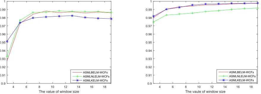
Experiment #3: In this experiment, we assess the effects of the window size for the proposed spectral-spatial classifiers,
ASMLBELM-WCFs, ASMLNLELM-WCFs and
ASMLKELM-WCFs, and the results are given in Fig. 4. As seen, the results of the proposed methods are not very good when the window size is too small, i.e. less than 5. However, the results are much improved when the window size is larger than 10. This shows the generalization for achieving the good performance of the proposed spectral-spatial classifiers. For the convenience, the window size is set as 13 for both the Indian Pines data set and the Pavia University data set in the following experiments if there is no special mention.
D. Experiment Results and Discussions
In this subsection, the classification results on the two data sets are evaluated and shown in Table 1 and Table 2, where our proposed six approaches are benchmarked with eight others. In these two tables, we also show the index of the classes and the numbers of training samples and testing samples for each class. For the Indian Pines data set and the Pavia University data set, we set 10% and 9% for training, respectively, and the remaining samples are used for testing.
As can be seen in Table 1 and Table 2, the proposed ASMLBELM, ASMLNLELM and ASMLKELM approaches yield higher accuracy than BELM, NLELM and KELM, respectively. The performance of the three proposed spectral classifiers are improved dramatically when the spatial information (WCFs) are added. Compared with other spectral spatial classifiers such as the SVM-CK and the SMLR-SpATV,
our proposed ASMLBELM-WCFs, ASMLNLELM-WCFs and ASMLKELM-WCFs have produced higher classification accuracy, especially ASMLNLELM-WCFs for the Indiana Pines data set and ASMLKELM-WCFs for the Pavia University data set. Visual comparison of the classification results is also shown in Fig. 5 and Fig. 6 for the results from the two data sets as well as the ground reference map, which again validates the efficacy of the proposed approaches.
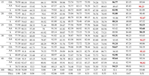
E. Experiments with Different Numbers of Training Samples
The performances of the proposed six methods are further evaluated under different numbers of training samples, where the total number of training samples is respectively chosen as 5, 10, 15, 20, 25, 30, 35 and 40 from each class. If the selected number exceeds half of the total pixels in one particular class, we only choose 50% of the samples for training in that class. For the two data sets, relevant results are given in Table 3 and Table 4 for comparison.
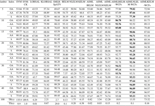
[image:9.612.86.526.551.710.2]As seen from Table 3 and Table 4, with the change of the number of training samples, the classification accuracy of the three spectral classifiers is always better than those from BELM, NLELM and KELM. These three spectral-spatial classification algorithms can also always achieve best performances among all the methods despite of the number of training samples used. Apparently, the performances of the proposed six methods are improved with increased number of training samples. However, when the number of training samples is over 20, the classification accuracy becomes almost saturated and does not change significantly. What is more interesting, when we use only 5 samples for training, the best classification accuracy the proposed methods can achieve exceeds 75% for both the two data sets, which outperform all other benchmarking methods at least 8%. On the other hand, it is worth noting that the classification accuracy of BELM surprisingly decreases when the number of training samples increases in most cases. This is because the ill-posed problem is particularly sensitive in BELM, and there may be different optimal numbers of hidden neurons for cases with various numbers of training samples. This can be also seen in Fig. 3, however, the proposed ASMLBELM and ASMLBELM-WCFs well alleviate this problem.
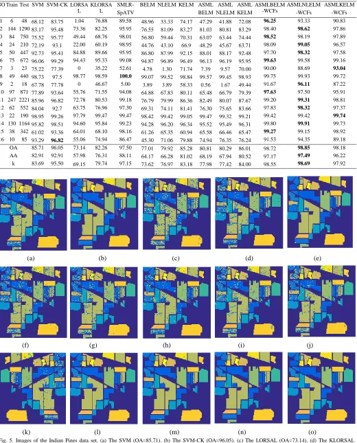
TABLE 1.CLASSIFICATION ACCURACY USING 10% OF THE LABELED SAMPLES PER CLASS FOR THE INDIAN PINES DATA SET (THE BEST RESULTS ARE BOLDED).
NO Train Test SVM SVM-CK LORSA L
KLORSA L
SMLR- SpATV
BELM NLELM KELM ASML BELM
ASML NLELM
ASML KELM
ASMLBELM -WCFs
ASMLNLELM -WCFs
ASMLKELM -WCFs 1 6 48 68.12 83.75 1.04 76.88 89.58 48.96 33.33 74.17 47.29 41.88 72.08 96.25 93.33 90.83 2 144 1290 83.17 95.48 73.36 82.25 95.95 76.55 81.09 83.27 81.03 80.81 83.29 98.40 98.62 97.86 3 84 750 75.52 95.77 49.44 68.76 98.01 56.80 59.44 70.31 63.07 63.44 74.44 98.52 98.19 97.89 4 24 210 72.19 93.1 22.00 60.19 98.95 44.76 43.10 66.9 48.29 45.67 63.71 98.09 99.05 96.57 5 50 447 92.73 95.41 84.88 89.66 95.95 86.80 87.99 92.15 88.01 88.17 92.48 97.70 98.32 97.58 6 75 672 96.06 99.29 94.43 95.33 99.08 94.87 96.89 96.49 96.13 96.19 95.95 99.63 99.58 99.16 7 3 23 75.22 77.39 0 35.22 52.61 4.78 1.30 71.74 7.39 9.57 70.00 90.00 88.69 93.04
8 49 440 98.73 97.5 98.77 98.59 100.0 99.07 99.52 98.84 99.57 99.45 98.93 99.75 99.93 99.72 9 2 18 67.78 77.78 0 46.67 5.00 3.89 3.89 58.33 0.56 1.67 49.44 91.67 96.11 87.22 10 97 871 77.89 93.64 55.76 71.55 94.08 64.88 67.83 80.11 65.48 66.79 79.39 97.63 97.50 95.91 11 247 2221 85.96 96.82 72.78 80.53 99.18 76.79 79.99 86.36 82.49 80.07 87.67 99.20 99.31 98.81 12 62 552 84.04 92.7 63.75 76.96 97.30 69.31 74.11 81.41 76.30 75.65 83.66 97.83 98.32 97.37 13 22 190 98.95 99.26 97.79 99.47 99.47 98.42 99.42 99.05 99.47 99.32 99.21 99.42 99.42 99.74
14 130 1164 95.82 98.51 94.60 95.84 99.23 94.28 96.20 96.34 95.52 95.49 96.31 99.80 99.91 99.73 15 38 342 61.02 93.36 64.01 68.10 98.16 61.26 65.35 60.94 65.58 66.46 65.47 99.27 99.15 98.92 16 10 85 93.29 96.82 55.06 74.94 86.47 45.30 71.06 79.88 74.94 76.35 76.24 91.53 94.35 89.18
OA 85.71 96.05 73.14 82.26 97.50 77.01 79.92 85.28 80.81 80.29 86.01 98.72 98.85 98.18 AA 82.91 92.91 57.98 76.31 88.11 64.17 66.28 81.02 68.19 67.94 80.52 97.17 97.49 96.22 k 83.69 95.50 69.15 79.74 97.15 73.62 76.97 83.18 77.98 77.42 84.00 98.55 98.69 97.92
(a) (b) (c) (d) (e)
(f) (g) (h) (i) (j)
(k) (l) (m) (n) (o)
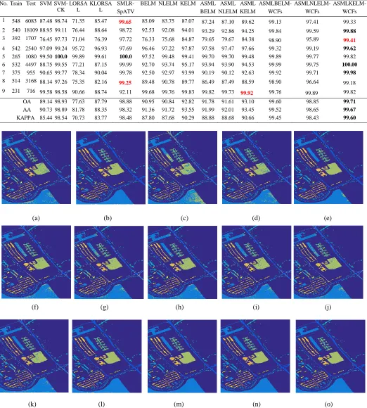
[image:10.612.49.569.67.712.2] [image:10.612.43.569.74.700.2]TABLE 2.CLASSIFICATION ACCURACY USING 9% OF THE LABELED SAMPLES PER CLASS FOR THE PAVIA UNIVERSITY DATA SET (THE BEST RESULTS ARE BOLDED).
No. Train Test SVM SVM-CK
LORSA L
KLORSA L
SMLR- SpATV
BELM NLELM KELM ASML BELM
ASML NLELM
ASML KELM
ASMLBELM- WCFs
ASMLNLELM- WCFs
ASMLKELM- WCFs 1 548 6083 87.48 98.74 71.35 85.47 99.65 85.09 83.75 87.07 87.24 87.10 89.62 99.13 97.41 99.33 2 540 18109 88.95 99.11 76.44 88.64 98.72 92.53 92.08 94.01 93.29 92.86 94.25 99.84 99.59 99.88
3 392 1707 76.45 97.73 71.04 76.39 97.72 76.33 75.68 84.87 79.65 79.67 84.38 98.90 95.89 99.41
4 542 2540 97.09 99.24 95.72 96.93 97.69 96.46 97.22 97.87 97.58 97.47 97.66 99.32 99.19 99.62
5 265 1080 99.50 100.0 99.89 99.61 100.0 97.52 99.48 99.41 99.70 99.70 99.48 99.89 99.77 99.82 6 532 4497 88.75 99.55 77.21 87.15 99.99 92.70 93.74 95.17 93.94 93.90 94.53 99.99 99.75 100.00
7 375 955 90.65 99.77 78.34 90.04 99.78 92.50 92.97 93.99 90.19 90.12 92.63 99.92 99.71 99.98
8 514 3168 88.14 97.26 75.35 82.16 99.25 89.48 90.78 89.77 86.49 87.49 88.59 98.90 96.64 99.18 9 231 716 99.58 98.58 90.66 88.74 92.11 99.68 99.76 99.83 99.82 99.73 99.92 99.76 99.89 99.82 OA 89.14 98.93 77.63 87.79 98.88 90.95 90.84 92.82 91.78 91.61 93.10 99.60 98.85 99.71
AA 90.73 98.89 81.78 88.35 98.32 91.36 91.72 93.55 91.99 92.01 93.45 99.52 98.65 99.67
KAPPA 85.44 98.54 70.73 83.77 98.48 87.80 87.68 90.29 88.88 88.68 90.66 99.45 98.43 99.60
(a) (b) (c) (d) (e)
(f) (g) (h) (i) (j)
[image:11.612.49.568.66.657.2]
(k) (l) (m) (n) (o)
Fig. 6. Images of the Pavia University data set. (a) The SVM (OA=89.14). (b) The SVM-CK (OA=98.93). (c) The LORSAL (OA=77.63). (d) The KLORSAL (OA=87.79). (e) The SMLR-SpATV (OA=98.88). (f) The BELM (OA=90.87). (g) The NLELM (OA=90.80). (h) The KELM (OA=92.82). (i) The ASMLBELM (OA=92.06). (j) The ASMLNLELM (OA=91.71). (k) The ASMLKELM (OA=93.07). (l) The ASMLBELM-WCFs (OA=99.46). (m) The ASMLNLELM-WCFs (OA=99.44). (n) The ASMLKELM-WCFs (OA=99.69) with 9% training samples. (o) The ground reference map.
In Table 3 and Table 4, we also illustrate the execution time (including the training time and testing time) of the six proposed algorithms and other methods when using 100
[image:11.612.46.568.69.649.2]sets. Though most of the methods take more time for training than testing, there are exceptional cases such as SMLR-SpATV. Also some methods take more time in Indian Pines dataset, while others take more in the Pavia University dataset. That is affected by both the volume and the content of the dataset when the corresponding classifiers were trained and tested. All in all, the proposed approaches are among the medium group for training and the fastest groups for testing.
From Table 3 and Table 4, for the Indian Pines data sets and Pavia University data sets, the three proposed spectral algorithms, i.e. ASMLBELM, ASMLBELM and ASMLKELM need more time consumption than BELM, NLELM and KELM, respectively, yet they consume less time than SVM. In Indian
Pines data set, the proposed ASMLBELM-WCFs and ASMLNLELM-WCFs algorithms consume less time than SVM-CK and SMLR-SpATV. Although the proposed ASMLEKELM-WCFs consume more time than SMLR-SpATV, it needs less time than SVM-CK. In Pavia University data sets, the three proposed spectral-spatial algorithms have less consuming time than SVM-CK and SMLR-SpATV. In summary, the proposed six classification methods achieve very good performances, especially the three spectral-spatial classification algorithms, where the computational efficiency is not bad in comparison to its peers although it can be further improved.
TABLE 3.CLASSIFICATION ACCURACY (%) UNDER DIFFERENT NUMBERS OF TRAINING SAMPLES FOR THE INDIAN PINES DATA SET (THE BEST RESULTS ARE BOLDED).
TABLE 4.CLASSIFICATION ACCURACY (%) UNDER DIFFERENT NUMBERS OF TRAINING SAMPLES FOR THE PAVIA UNIVERSITY DATA SET (THE BEST RESULTS ARE BOLDED).
Numbe r
Index SVM SVM-CK
LORSAL KLORSAL SMLR- SpATV
BELM NLELM KELM ASML BELM
ASML NLELM
ASML KELM
ASMLBELM -WCFs
ASMLNLEL M -WCFs
ASMLKELM -WCFs
5 OA 56.75 63.85 47.58 56.5 65.87 57.75 61.71 62.86 61.22 65.88 63.61 75.68 71.48 70.52 AA 69.79 72.74 47.3 67.48 74.82 67.36 72.26 72.87 71.63 73.39 72.80 80.95 76.81 78.19
k 47.58 55.26 35.93 55.53 57.58 48.56 52.88 53.94 52.58 57.57 54.48 69.39 64.19 62.98 10 OA 66.31 73.82 50.19 62.49 76.23 57.75 69.41 69.21 72.67 70.92 71.01 83.51 76.43 81.30
AA 75.47 80.64 50.09 71.65 79.95 64.96 76.51 78.98 78.05 78.08 79.17 86.60 81.53 86.69
k 57.79 67.06 38.68 53.81 69.70 48.08 61.63 61.68 65.33 63.40 63.64 78.79 70.08 76.04 Number Index SVM
SVM-CK
LORSAL KLORSAL SMLR- SpATV
BELM NLELM KELM ASML BELM
ASML NLELM
ASML KELM
ASMLBELM -WCFs
ASMLNLEL M-WCFs
ASMLKELM -WCFs 5 OA 53.84 57.30 43.53 57.34 69.67 42.22 50.94 54.68 53.60 54.86 54.95 77.96 79.82 72.94
AA 67.36 70.78 53.28 68.89 81.98 54.75 65.52 66.6 67.73 68.23 67.61 87.09 87.66 81.85 k 48.54 52.52 37.84 52.59 66.16 36.19 45.62 49.4 48.33 49.57 49.69 75.28 77.30 69.55 10 OA 62.85 69.94 49.05 65.48 78.60 43.04 58.80 63.45 60.24 61.39 63.60 86.78 86.22 81.73 AA 74.01 80.45 62.77 75.99 88.22 55.12 72.85 75.63 74.04 74.20 75.38 92.76 92.52 89.13
k 58.37 66.30 43.7 61.38 76.03 36.92 54.21 59.11 55.57 56.72 59.32 85.08 84.46 79.40 15 OA 69.77 78.15 55.3 68.04 83.59 42.39 61.64 67.87 62.76 64.67 68.86 89.81 90.06 87.04 AA 80.10 86.66 67.06 78.49 91.02 52.42 75.13 79.66 76.01 77.83 79.71 94.62 94.71 93.10
k 66.07 75.38 50.18 64.23 81.48 35.72 57.27 63.99 58.27 60.42 65.09 88.46 88.74 85.34 20 OA 72.54 80.86 58.83 72.27 86.73 38.71 65.24 71.34 64.05 67.25 71.62 92.00 92.30 88.93 AA 81.77 88.35 69.62 81.62 93.10 45.46 77.86 81.67 77.09 79.55 81.57 95.77 96.03 94.30 k 69.06 78.41 53.96 68.85 85.00 31.54 61.06 67.79 59.71 63.22 68.06 90.90 91.25 87.47 25 OA 74.89 83.52 60.16 72.92 87.82 30.80 66.57 72.04 62.07 68.93 74.21 92.77 93.28 91.82 AA 83.64 90.12 70.98 82.99 93.81 34.88 79.60 82.86 74.54 81.04 83.78 96.24 96.65 95.35
k 71.74 81.36 55.4 69.58 86.20 22.64 62.59 68.59 57.35 65.09 70.97 91.78 92.36 90.70 30 OA 75.10 85.31 61.89 73.93 89.31 16.60 67.15 75.24 44.70 69.87 76.52 94.52 94.12 92.47 AA 84.16 91.88 71.16 82.95 94.48 14.68 80.20 84.5 52.11 81.52 85.52 97.14 96.96 96.15
k 71.97 83.35 57.35 70.65 87.85 7.37 63.29 72.05 37.77 66.10 73.51 93.76 93.31 91.43 35 OA 76.74 87.22 63.7 75.09 89.67 40.01 68.75 75.73 66.67 71.41 76.99 95.41 95.53 93.30 AA 85.15 92.89 72.89 84.05 95.06 46.22 80.65 85.55 78.74 82.88 85.59 97.46 97.64 96.37 k 73.74 85.49 59.28 71.92 88.28 32.63 65.05 72.64 62.49 67.82 74.00 94.75 94.89 92.36 40 OA 78.47 88.9 64.25 75.93 90.74 53.93 70.19 76.58 71.33 72.30 77.67 95.70 96.09 94.57 AA 86.01 93.75 73.76 83.57 95.20 64.58 81.31 86.09 82.30 82.62 85.96 97.56 97.84 96.97
k 75.64 87.38 59.91 72.77 89.45 48.34 66.61 73.55 67.67 68.77 74.74 95.08 95.53 93.79 100 TR(s) 135.9 189.9. 0.29 2.21 2.7 0.13 1.75 6.15 0.82 3.54 12.28 10.9 13.55 73.32
[image:12.612.60.559.245.587.2] [image:12.612.50.562.628.738.2]15 OA 70.58 80.18 55.61 66.11 80.96 59.98 73.74 72.77 73.59 74.26 72.71 86.77 83.15 85.84 AA 78.42 84.65 53.82 74.39 87.57 63.74 79.77 82.13 79.29 79.77 80.63 89.67 85.83 90.23
k 62.98 74.69 44.53 53.93 75.82 50.12 66.72 66.05 66.52 67.30 65.53 82.98 78.25 81.89 20 OA 72.45 84.2 59.27 70.6 85.20 61.94 75.04 76.75 73.91 76.76 76.95 91.00 85.14 90.40
AA 79.38 87.53 56.6 76.41 89.22 64.67 80.79 83.38 80.15 81.51 83.59 91.86 87.75 92.67
k 65.07 79.63 48.3 59.52 81.00 52.36 68.35 70.48 67.04 70.34 70.79 88.24 .80.80 87.52 25 OA 73.90 89.05 58.33 71.44 88.48 59.67 77.56 78.95 77.56 78.09 79.02 92.33 88.17 92.53
AA 81.35 90.31 57.49 78 91.34 61.82 82.39 84.92 81.51 82.09 84.56 93.42 89.76 93.68
k 67.04 85.71 47.56 61.02 85.14 50.07 71.33 73.15 71.24 71.92 73.21 89.98 84.60 90.19
30 OA 77.70 89.21 60.69 73.64 91.02 61.35 78.87 78.53 78.36 79.90 80.37 93.31 90.23 93.03 AA 82.45 90.33 60.16 78.87 92.55 61.53 83.58 84.91 82.44 83.60 85.99 93.95 91.28 94.27
k 71.38 85.87 50.47 68.29 88.26 51.76 72.95 72.72 72.26 74.15 74.94 91.24 87.24 90.86 35 OA 75.19 90.42 61.71 75.16 91.55 59.01 79.66 81.09 78.44 79.55 81.32 94.67 91.13 94.19 AA 82.99 91.8 61.86 79.33 93.36 59.09 84.58 86.33 82.79 83.46 86.71 94.95 92.33 95.15
k 68.69 87.48 51.68 67.11 88.97 49.28 73.97 75.78 72.49 73.73 76.11 92.98 88.41 92.36 40 OA 77.09 91.9 63.15 76.92 91.68 56.78 80.21 82.53 79.77 80.91 82.65 95.64 92.41 95.54 AA 83.02 92.47 63.3 80.81 92.40 55.91 84.12 87.32 83.27 84.97 87.59 95.41 92.91 96.02 k 70.73 89.36 53.3 70.85 89.13 46.73 74.48 77.53 74.01 75.50 77.75 94.23 90.01 94.11 100 TR(s) 39.30 76.89 0.12 0.88 1.09 0.40 0.84 4.03 2.77 3.27 6.22 32.1 37.28 53.80
TS(s) 1.98 2.60 0.04 1.42 92.06 0.95 0.98 1.0 0.31 0.32 0.53 0.31 0.67 0.51
F. Extension of Experiments
In this subsection, we further evaluate the performance of the proposed three classifiers, in comparison to other spectral- spatial methods, including BELM/NLELM/KELM with weighted composite features (WCFs) i.e. BELM-WCFs, NLELM-WCFs and KELM-WCFs respectively, KELM with Gabor (KELM-Gabor) filter [28] and KELM with local binary pattern (KELM-LBP) [26]. In addition to the Indian Pines and Pavia University datasets, we also take the Salinas dataset for extended testing using 1% samples per class for training.
The parameter settings of these benchmarking approaches are given below. For BELM-WCFs, NLELM-WCFs and KELM-WCFs, the width/height of the neighborhood window, wopt, is all set to 13. For BELM-WCFs, the number of hidden neuron, L, is set to 450 for Indian Pines dataset, 1100 for Pavia University and Salinas datasets. For NLELM-WCFs, the number of hidden neuron is set to 1000 for Indian Pines dataset, 1100 for Pavia University and Salinas datasets. For KELM-WCFs, the parameters C and σ are automatically tuned using three-folds cross validations. For KELM-LBP and KELM-Gabor, they are applied on the first 30 principal components of the dataset as features. According to [26], the parameters r (a circle of radius centered at the center pixel) and nr (the numbers of neighboring pixels) of LBP are set to 2 and 8, respectively, and the parameter bw (the frequency bandwidth) of KELM-Gabor is set to 5.
For parameter λ= 2𝑎 in the proposed three approaches, we
set a = −16 for both ASMLBELM-WCFs and
ASMLNLELM-WCFs, while for ASMLKELM-WCFs we set 𝑎 = −28 in all the three datasets. The number of hidden neurons is set to 1100 for ASMLBELM-WCFs and ASMLNLELM-WCFs for the Salinas dataset. Relevant results are given in Table 5 for comparison.
Using 1% samples per class for training, the experimental results from our proposed methods and the aforementioned benchmarking approaches are compared in Table 5. From Table 5, we can see that the proposed three spectral-spatial methods produce improved classification accuracy than the original ones respectively even combined with WCFs. On the other hand, all the proposed three spectral-spatial methods yield higher classification accuracy than KELM-Gabor. Furthermore, compared with KELM-LBP, the proposed three spectral-spatial methods have comparable or slightly better classification results in the Salinas dataset, and better classification results in Indian Pines and Pavia University datasets.
In Table 6, we further compare our proposed methods with the well-known locality adaptive discriminant analysis (LADA) [10] and multitask joint sparse representation and stepwise MRF optimization (MSMRF) [16] approaches. The classification results of LADA and MSMRF on the Indian Pines and Pavia University datasets are directly taken from [10] and [16], respectively. The experiment settings are the same as [10] and [16]. It should be noting that as stated in [10], when comparing with LADA, we randomly sample 5% points as training set, and 30% of the remaining data as test set. From Table 6, again it clearly shown that the proposed methods outperform both the MSMRF and LADA.
TABLE 5.RESULTS OF CLASSIFICATION ACCURACY USING 1% OF THE SAMPLES PER CLASS FOR TRAINING (THE BEST RESULTS ARE BOLDED)
Datasets Index KELM-Gabor KELM-LBP BELM- WCFs
NLELM- WCFs
KELM- WCFs
ASMLBELM- WCFs
ASMLNLELM- WCFs
ASMLKELM- WCFs Indian
Pines
OA 71.30 84.45 86.14 87.32 86.18 89.78 90.10 86.64
[image:13.612.54.563.48.310.2] [image:13.612.57.554.692.742.2]kappa 66.97 82.30 84.19 85.55 84.24 88.36 88.74 84.78
Pavia University
OA 87.73 92.22 88.62 94.27 96.52 96.42 95.28 96.78
AA 81.08 85.45 74.61 89.93 93.74 92.24 91.80 94.57
kappa 83.31 89.61 84.78 92.33 95.37 95.24 93.72 95.72
Salinas OA 95.65 98.82 98.15 96.69 98.25 98.92 98.16 98.31
AA 96.48 98.87 98.57 98.32 98.84 99.25 98.93 98.79
kappa 95.15 99.03 97.94 96.31 98.05 98.79 97.95 98.12
TABLE 6.COMPARISON WITH OTHER METHODS (THE BEST RESULTS ARE BOLDED).
V.CONCLUSION
In this paper the augmented spare multinomial logistic extreme learning machine (ASMLELM) is proposed to alleviate the ill-posed problem of ELM, which has resulted in three spectral algorithms and three spectral-spatial methodologies for the classification of HSI. By combining the proposed ASMLELM with the weighted composite features (WCFs), the three spectral-spatial methods can effectively extract the spatial information for improved classification than the conventional ELM. In addition to derive the lower bound of the proposed method by a rigorous mathematical proof, comprehensive experimental results on three well-known HSI dataset have also validated the superior performance of the proposed algorithms in terms of improved classification accuracy and inherited efficiency from ELM.
For future work, we will focus on improving the classification accuracy of the proposed ASMLELM by resorting to the extended multi-attribute profiles [56-57] (EMAPs) method.
REFERENCES
[1] Y. Zhou, J. Peng, C. L. P. Chen, “Extreme learning machine with composite kernels for hyperspectral image classification,” IEEE J. Sel. Top. Appl. Earth Obs. Remote Sens., vol. 8, no. 6, pp. 2351-2360, 2015.
[2] A. Plaza, J. A. Benediktsson, J. W. Boardman, et al, “Recent advances in techniques for hyperspectral image processing,” Remote Sens. Environ., vol. 113, pp. S110-S122, 2009.
[3] Hughes G, “On the mean accuracy of statistical pattern recognizers,” IEEE Trans. Inf. Theory, vol. 14, no. 1, pp. 55-63, 1968.
[4] J. Li, P. R. Marpu, A. Plaza, et al, “Generalized composite kernel frame work for hyperspectral image classification,” IEEE Trans. Geosci. Remote Sens., vol. 51, no. 9, pp. 4816-4829, 2013.
[5] T. Qiao, J. Ren et al, “Effective denoising and classification of hyperspectral images using curvelet transform and singular spectrum analysis,” IEEE Trans. Geosci. Remote Sens., vol. 55, no. 1, pp. 119-133, 2017.
[6] J. Zabalza, J. Ren, J. Zheng, J. Han, H. Zhao, S. Li, and S. Marshall, “Novel two dimensional singular spectrum analysis for effective feature extraction and data classification in hyperspectral imaging,” IEEE Trans. Geosci. Remote Sens., vol. 53, no. 8, pp. 4418-4433, 2015.
[7] T. Qiao, J. Ren, C. Craigie, Z. Zabalza, C. Maltin, S. Marshall, “Singular spectrum analysis for improving hyperspectral imaging based beef eating quality evaluation,” Comput. Electron. Agric., 2015.
[8] J. Zabalza, J. Ren, Z. Wang, H. Zhao, J. Wang, and S. Marshall, “Fast implementation of singular spectrum analysis for effective feature extraction in hyperspectral imaging,” IEEE J. Sel. Top. Appl. Earth Obs. Remote Sens., vol. 8, no. 6, pp. 2845-53, 2015.
[9] F. Melgani, L. Bruzzone, “Classification of hyperspectral remote sensing images with support vector machines,” IEEE Trans. Geosci. Remote Sens., vol. 42, no. 8, pp. 1778-1790, 2004.
[10] Q. Wang, Z. Meng, X. Li,“Locality adaptive discriminant analysis for spectral–spatial classification of hyperspectral images,” IEEE Geosci. Remote Sens. Lett,vol. 14, no. 11, pp. 2077-2081, 2017.
[11] J. Zabalza, J. Ren, J. Zheng, H. Zhao, C. Qing, Z. Yang, P. Du and S. Marshall, “Novel segmented stacked autoencoder for effective dimensionality reduction and feature extraction in hyperspectral imaging,”
Neurocomputing, vol. 185, pp. 1-10, 2016.
[12] J. Ren, Z. Zabalza, S. Marshall and J. Zheng, “Effective feature extraction and data reduction with hyperspectral imaging in remote sensing,” IEEE Signal Proc. Mag., vol. 31, no. 4, pp. 149-154, 2014.
[13] J. Zabalza, J.-C. Ren, J. Ren, Z. Liu, and S. Marshall, “Structured cova ciance principle component analysis for real-time onsite feature extraction and dimensionality reduction in hyperspectral imaging,” Appl. Opt., vol. 53, no. 20, pp. 4440-4449, 2014.
[14] J. Zabalza, J. Ren, M. Yang, Y. Zhang, J. Wang, S. Marshall, J. Han, “Novel Folded-PCA for Improved Feature Extraction and Data Reduction with Hyperspectral Imaging and SAR in Remote Sensing,” ISPRS J. Photogramm. Remote Sens, vol. 93, no. 7, pp. 112-122, 2014.
[15] Y. Yuan, J. Lin, Q. Wang, “Hyperspectral image classification via multitask joint sparse representation and stepwise MRF optimization,”
IEEE Trans. Cybern, vol. 46, no. 12, pp. 2966-2977, 2016.
[16] Q. Wang, J. Lin, Y. Yuan, “Salient band selection for hyperspectral image classification via manifold ranking,”IEEE Trans. Neural Netw. Learn. Syst, vol. 27, no. 6, pp. 1279-1289, 2016.
[17] G. B. Huang, Q. Y. Zhu, C. K. Siew, “Extreme learning machine: theory and applications,” Neurocomputing, vol. 70, no. 1, pp. 489-501, 2006. [18] F. Cao, Z. Yang, J. Ren, M. Jiang, W-K Ling, “Linear vs Nonlinear
Extreme Learning Machine for Spectral-Spatial Classification of Hyperspectral Image,” Sensors., vol. 17, no. 11, pp. 2603, 2017. 10% training samples, remaining for testing 5% training samples, 30% of remaining for testing
MSMRF [16]
ASMLBELM- WCFs
ASMLNLELM- WCFs
ASMLKELM- WCFs
LADA [10]
ASMLBELM- WCFs
ASMLNLELM- WCFs
ASMLKELM- WCFs Indian
Pines
OA 92.11 98.86 98.61 98.53 91.75 97.46 97.13 96.97
AA 94.86 97.95 97.75 97.92 85.09 95.62 96.45 96.36
k - 98.70 98.41 98.33 90.56 97.11 96.73 96.55
Pavia University
OA 92.52 99.44 98.66 98.47 89.66 98.97 98.06 97.20
AA 95.41 99.01 97.76 97.38 88.23 97.94 96.65 95.86