Theses Thesis/Dissertation Collections
12-8-2014
Temporal Signature Modeling and Analysis
Jiangqin Sun
Follow this and additional works at:http://scholarworks.rit.edu/theses
This Dissertation is brought to you for free and open access by the Thesis/Dissertation Collections at RIT Scholar Works. It has been accepted for inclusion in Theses by an authorized administrator of RIT Scholar Works. For more information, please [email protected].
Recommended Citation
by
Jiangqin Sun
B.S. Soochow University, 2007 M.S. Harbin Institute of Technology, 2009
A dissertation submitted in partial fulfillment of the requirements for the degree of Doctor of Philosophy
in Imaging Science
Chester F. Carlson Center for Imaging Science College of Science
Rochester Institute of Technology
December 8, 2014
Signature of the Author
Accepted by
ROCHESTER INSTITUTE OF TECHNOLOGY ROCHESTER, NEW YORK
CERTIFICATE OF APPROVAL
Ph.D. DEGREE DISSERTATION
The Ph.D. Degree Dissertation of Jiangqin Sun has been examined and approved by the dissertation committee as satisfactory for the
dissertation required for the Ph.D. degree in Imaging Science
Dr. David Messinger, Dissertation Advisor
Dr. Tony Harkin, Committee Member
Dr. Joel Kastner, Committee Member
Dr. Carl Salvaggio, Committee Member
A vast amount of digital satellite and aerial images are collected over time, which calls for techniques to extract useful high-level information, such as recognizable events. One part of this thesis proposes a framework for streaming analysis of the time series, which can recognize events without supervision and memorize them by building the temporal contexts. The memorized historical data is then used to predict the future and detect anomalies. A new incremental clustering method is proposed to recognize the event without training. A memorization method of double localization, including relative and absolute localization, is proposed to model the temporal context. Finally, the predictive model is built based on the method
of memorization. The “Edinburgh Pedestrian Dataset”, which offers about 1000
observed trajectories of pedestrians detected in camera images each working day for several months, is used as an example to illustrate the framework.
The Ph.D. study at RIT was a great experience for me. During the last few
years, I was offered a lot of opportunities to learn and grow. I feel grateful to all
the people I meet at RIT, who altogether makes RIT a warm place to stay.
First, I would like to thank my advisor, Dr. David Messinger, for his constant support, encouragement, and patience. He has been a wonderful advisor in balancing
guidance and giving freedom to students, which allows us to work effectively and
creatively. This work would not be possible without his mentoring.
I also would like to thank my committee members: Dr. Tony Harkin, Dr. Carl Salvaggio and Dr. Joel Kastner for taking the time to provide their support and give me valuable feedback on my work.
I would like to thank Dr. Michael Gartley for his kindness to teach me DIRSIG. Many thanks to Jason Faulring for helping me setting up the parking lot experiment. I thank Rolando Raqueño, Andrew Scott, and Nina Raqueño for their discussion, feedback, and support in the parking lot modeling in DIRSIG.
I would like to all the CIS admin staff, who makes things so well organized. In
particular I’d like to thank Cindy Schultz, Sue Chan, Marilyn Lockwood, and Joyce French.
It would be very difficult for me to complete the Ph.D. study without the
sup-port from friends, roommates, and fellow graduate students. Special thanks to Dr. Weihua Sun, Lin Chen, Dr. Yujie Qiu, Wei Yao and Fan Jiang for their support and companion through the toughest first year study in U.S..
1 Introduction 1
1.1 Temporal Signature Modeling in DIRSIG . . . 2
1.2 Temporal signature analysis . . . 6
1.3 Summary . . . 7
2 DIRSIG Simulation 9 2.1 The understanding of DIRSIG . . . 9
2.1.1 First principles based working mechanism of DIRSIG . . . 10
2.1.2 Input files of DIRSIG . . . 13
2.1.2.1 The .scene file . . . 14
2.1.2.2 The .atm file . . . 17
2.1.2.3 The .platform file . . . 18
2.1.2.4 The .ppd file . . . 19
2.1.2.5 The .tasks file . . . 19
2.2 Timing in DIRSIG . . . 20
2.3 Process models . . . 22
3 Temporal Signature Modeling in DIRSIG 24 3.1 Work flow . . . 24
3.2 Process models driving per facet property changing . . . 27
3.2.1 UV mapping . . . 28
3.2.2 Two-tanks thermal model . . . 35
3.3.2 PARKVIEW incorporated DIRSIG simulation results . . . 46
3.3.3 Experiment: statistical description extraction of parking lots . 51 3.3.3.1 Experiment data processing . . . 52
3.3.3.2 Experiment Result . . . 59
3.3.4 Summary . . . 62
4 Temporal Signature Analysis 64 4.1 Problem statement . . . 64
4.1.1 Kalman filter . . . 65
4.1.2 ARIMA . . . 68
4.1.3 Human cognitive system . . . 68
4.2 Proposed methods . . . 69
4.2.1 Preprocess the time series . . . 71
4.2.1.1 Missing data estimation . . . 71
4.2.1.2 Outlier removal and noise reduction . . . 72
4.2.2 Knowledge acquisition . . . 73
4.2.3 Event recognition . . . 73
4.2.3.1 Euclidean distance . . . 75
4.2.3.2 k-means classification . . . 75
4.2.3.3 RX anomaly detection . . . 76
4.2.3.4 TAD anomaly detection . . . 76
4.2.3.5 Fourier filter . . . 77
4.2.4 Event memorization . . . 78
4.2.5 Event prediction . . . 79
4.3 Data sets . . . 79
5 Recognition by incremental clustering of data streams 82 5.1 Review of related work . . . 83
5.2.3 Cluster descriptions . . . 93
5.2.4 Cluster data management and parameters . . . 96
5.2.5 Short-comes and possible solutions . . . 97
5.3 Result on simulated data . . . 98
5.3.1 Simulated Gaussian distributed data . . . 98
5.3.2 Simulated data set with arbitrary shapes . . . 99
5.4 Result on Edinburgh pedestrian dataset . . . 100
5.4.1 Incremental clustering of trajectories . . . 102
5.4.1.1 Review on clustering of trajectories . . . 102
5.4.1.2 Feature selection for trajectory clustering . . . 103
5.4.1.3 Results of the trajectory clustering . . . 104
5.4.2 Byproduct of clustering trajectories: extraction of semantic areas . . . 108
5.4.3 Incremental clustering of events . . . 110
5.4.3.1 Feature selection for event clustering and results . . . 114
6 Memorization and prediction 117 6.1 Memorization by double localization . . . 117
6.1.1 What to memorize and how? . . . 117
6.1.2 Related work . . . 119
6.1.2.1 Absolute localization: Exploring temporal associa-tion rules . . . 119
6.1.2.2 Relative localization: Modeling dynamics of trajec-tories or behaviors . . . 120
6.1.2.3 Similar terminology with different meanings . . . 121
6.1.3 Temporal map . . . 121
6.1.3.1 Temporal measures as sequences . . . 121
6.1.3.2 Temporal measures as maps . . . 123
6.2.2 Streaming prediction based on Edinburgh data . . . 132
7 Conclusion 137 8 Future work 139 A Results of streaming analysis of randomized data 155 A.1 Results of temporally randomized activities . . . 155
A.2 Results of temporally randomized events . . . 157
A.3 Comparison of the prediction results between real data and random-ized data . . . 158
A.4 Discussions . . . 160
B RIT twitter data 162 B.1 Data collection . . . 163
B.2 Preliminary data processing . . . 165
B.2.1 Preprocessing the data . . . 166
B.2.2 Result of event recognition . . . 167
B.2.2.1 Result of Euclidean distance . . . 169
B.2.2.2 Result of k-means classification . . . 172
B.2.2.3 Result of RX detector . . . 172
B.2.2.4 Result of TAD anomaly detection . . . 174
B.2.2.5 Result of Fourier filter . . . 177
B.2.2.6 Result comparison . . . 179
B.2.3 Event content understanding . . . 181
B.2.3.1 Method . . . 181
B.2.3.2 Result . . . 183
1.1 Midland Scene . . . 4
1.2 Problem structure . . . 8
2.1 Interactions between sub-models in DIRSIG[85] . . . 10
2.2 Sensor reaching radiance[91] . . . 12
2.3 DIRSIG XML input files . . . 13
2.4 The .scene file . . . 14
2.5 The .atm file . . . 18
2.6 Primary timing in DIRSIG . . . 21
2.7 Developed timing in DIRSIG . . . 22
3.1 Work flow chart of the process model . . . 25
3.2 Many-to-one Mapping . . . 28
3.3 An example image to be mapped onto geometry (“cameraman.tif” with size 256⇥256) . . . 29
3.4 Initial facet with 3 vertices . . . 30
3.5 Up sampled points on a facet in xy plane for drop-mapping method . 31 3.6 Up sampled facets with UV mapped information to half the plane . . 32
3.7 Up sampled facets with UV mapped information in higher resolution to the full plane . . . 32
3.8 Cylinder.obj . . . 33
3.9 Up sampled points on a facet for wrapmapping method . . . 34
3.13 Valve open/close time line . . . 38
3.14 Temperature and height of the water changing over time . . . 38
3.15 Two tanks mapped with temperature maps (Brightness is indicative of tank wall temperature.) . . . 40
3.16 RGB DIRSIG simulation of part of Midland scene . . . 40
3.17 DIRSIG simulation of part of Midland scene with two tanks process model included . . . 41
3.18 Probability Adjustment . . . 44
3.19 Preference of the parking spot . . . 47
3.20 Parking duration . . . 47
3.21 Distribution of parking lot occupancy . . . 48
3.22 Histogram of simulated parking duration . . . 48
3.24 Simulated occupancy of parking spots . . . 48
3.23 Simulated occupancy distribution of the parking lot . . . 49
3.25 Simulated status of the parking lot . . . 49
3.26 Number of arriving cars and leaving cars . . . 51
3.27 Original image of the parking lot . . . 52
3.28 Perspective transformed image of the parking lot . . . 52
3.29 Diagram of extracting the parking spot status . . . 54
3.30 Diagram of parking spot status initialization . . . 55
3.31 Vehicle class map . . . 56
3.32 Diagram of change detection of the parking spot status . . . 57
3.33 Empty parking spot . . . 58
3.34 Occupied parking spot . . . 58
3.35 Histogram of parking duration . . . 60
3.36 Parking lot occupancy over time . . . 61
3.37 Parking spot occupancy . . . 61
4.4 Human cognitive process . . . 68
4.5 Proposed method of temporal analysis . . . 69
4.6 Three key steps of the proposed method . . . 71
4.7 Example scene views of the Edinburgh Forum . . . 80
5.1 Workflow of incremental clustering . . . 86
5.2 Gaussian clustering . . . 90
5.3 Overlapped clusters . . . 91
5.4 Neighborhood of the new incoming point . . . 93
5.5 Merged clusters . . . 93
5.6 Finding the minimal number of rectangles . . . 95
5.7 Final description of clusters . . . 95
5.8 Result of incremental clustering on a data set with two synthetic Gaussian clusters . . . 98
5.9 Clustering result of RepStream on points with arbitrary shapes with different neighborhood connectivity value k and density scaler value ↵= 4.0 . . . 99
5.10 Result of incremental clustering on a data set with arbitrary shapes by the proposed GMD method . . . 99
5.11 Four different scenarios of the scene . . . 101
5.12 Four different scenarios of the scene with trajectories in different di-rection labelled . . . 101
5.13 The workflow of two step clustering . . . 102
5.14 Incremental clustering of trajectories with start points as features . . 105
5.15 The clusters with top 9 number of trajectories sharing the same start area within one hour of data . . . 106
5.18 The distribution of semantic areas . . . 110
5.19 The scene with semantic areas labeled . . . 110
5.20 The number of occurrences of all activities . . . 111
5.21 The cumulated summation of occurrence number of all activities . . . 112
5.22 Clustering structure with online and offline modes . . . 113
5.23 5 activities considered in this thesis . . . 114
5.24 Event clusters with raw numbers as features . . . 115
5.25 Event clusters with categorized features . . . 116
6.1 Temporal context models between events . . . 119
6.2 Segmentation of temporal measures in the form of sequences . . . 122
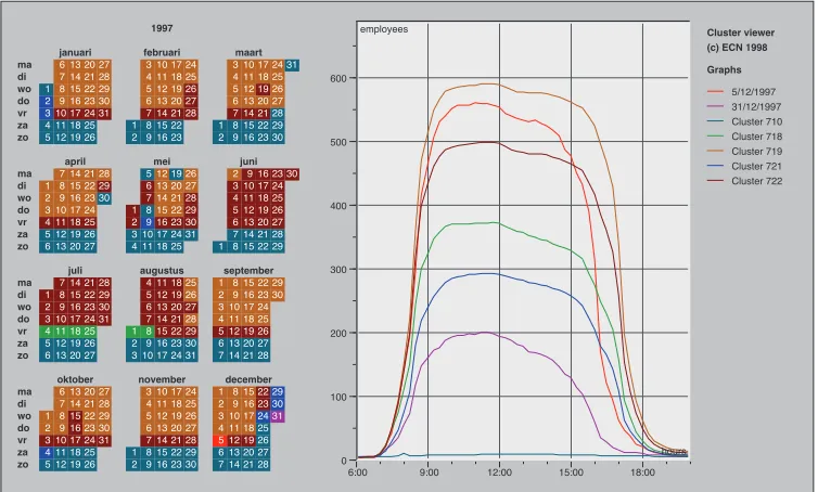
6.3 A calendar view of clusters of daily time series data on the number of employees present at ECN[104] . . . 124
6.4 Rectangular view[8] of a temporal clustering of meteorological time-oriented data from the Potsdam observation station. Changing the periodicity (denoted as decade) from 10 years (left) to six years (right) makes the temporal pattern of cluster 2 obvious[82]. . . 124
6.5 The temporal map of the occurrence number of activity 1 (from se-mantic area 2 to sese-mantic area 1) . . . 126
6.6 The temporal map of all 16 events with part zoomed-in . . . 127
6.7 The temporal map of event 4 . . . 127
6.8 Probability Matrix and support of events learned from Edinburgh dataset . . . 130
6.9 Prediction with probability matrix . . . 131
6.10 The predictive model with the probability matrix and the temporal map incorporated . . . 132
6.11 Stream prediction based on Edinburgh data . . . 133
6.12 The steaming analysis at 2009-9-23 8:10AM . . . 134
6.16 The prediction result during a long period when there are more
anoma-lies . . . 136
A.1 Event clusters with categorized features by using the activity tempo-rally randomized data . . . 156
A.2 Probability Matrix and support of events learned from the activity temporally randomized data . . . 157
A.3 Probability Matrix and support of events learned from the event tem-porally randomized data with random numbers of occurrences of each event . . . 157
A.4 Probability Matrix and support of events learned from the event tem-porally randomized data with real support . . . 158
A.5 Prediction results . . . 159
A.6 Hourly anomaly numbers of 4 datasets . . . 160
B.1 Tweets spatial distribution as heat map on RIT campus from Decem-ber 21, 2012 to DecemDecem-ber 28, 2012 (note: the higher density of tweets shows more red with the support from Google map API and twitter search API) . . . 164
B.2 Tweets temporal distribution on RIT campus from December 21, 2012 to December 28, 2012 . . . 165
B.3 Hourly tweet number . . . 166
B.4 Hourly tweet number with missing data estimated . . . 167
B.5 Percentage of variance along each principle component . . . 169
B.6 Percentage of variance carried in the first PC VS. the number of samples169 B.7 Result of Euclidean distance similarity method . . . 171
B.8 Classified PC space using k-means classifier with bar plot . . . 172
B.9 Classified time series using k-means classifier . . . 173
B.13 Result of TAD in time series space and TAD score . . . 176
B.14 Fourier filtered time series . . . 177
B.15 Difference between the original and filtered time series . . . 178
B.16 Result of anomaly detection by using Fourier filter . . . 178
B.17 The histogram of Euclidean distance and the threshold chosen (marked as a red line) . . . 179
B.18 The histogram of RX score and the threshold chosen (marked as a red line) . . . 180
B.19 The histogram of TAD score and the threshold chosen (marked as a red line) . . . 180
B.20 The histogram of differences between FFT filtered series and raw time series; the threshold is marked as a red line . . . 181
2.1 Example GDB file . . . 16
3.1 Scenarios of parking spot status change . . . 59
3.2 Result Accuracy analysis of the parking status extraction . . . 59
4.1 An example of event memory table . . . 78
B.1 Event recognition result comparison . . . 182
B.2 tweet content on an anomaly day . . . 184
Introduction
More than 150 Earth observation satellites are currently in orbit carrying sensors to monitor the earth and provide us a large number of valuable images[101]. Many companies and government agencies are still working on constructing next genera-tion satellites. For example, the ESA is developing five new missions called Sentinels to complement the capacities of the existing satellites in the next several years[2]. Besides, there are many airborne sensors available to take images of certain sites when required. During the 2012 summer, RIT (Rochester Institute of Technology) performed a large scale experiment in Avon area of Rochester which is named as SHARE2012. Several types of airborne sensors (including WASP, ALS-60, ProSpec-TIR VS, MircroHSI and PI Sensor[86]) flew over the site with targets set up in a designed way. The ground truth was measured and recorded along with the weather information. The collected data are shared around the world. The large amount of temporal digital satellite and aerial images calls for the corresponding development
in data processing techniques to combine and fuse the temporal data from different
sources in order to understand the data in a high level, such as extracting hidden events or activities. One part of the thesis will focus on building a generic framework to capture the temporal events from the data.
at RIT does not happen often, because such large scale experiments involve intense
amount of efforts and time. Besides, a lot of the data do not offer the “ground truth”,
which is required to test and validate the algorithm. The other part of the thesis will focus on generating temporal synthetic images by enhancing the capacity of a current tool called DIRISG (Digital Image and Remote Sensing Image Generation). In this thesis, we will illustrate temporal signature modeling in DIRSIG first to provide a method to generate the spatial-spectral-temporal synthetic remote sensing
images. This could further aid the research in temporal signature analysis by offering
the test data and their “ground truth”.
1.1 Temporal Signature Modeling in DIRSIG
the surface reflected radiances are determined to compute the sensor reaching ra-diances through the included MODTRAN model. DIRSIG can produce multi or
hyper-spectral remote sensing images between the bandpass 0.2 to 20mm with high
radiometric fidelity[31, 92]. In addition, DIRSIG also produces per-pixel “truth”, so many algorithm developers take this advantage of DIRSIG to validate their algo-rithms and make improvements.
However, except for vehicle moving, the solar and historical weather related short term temporal changing, DIRSIG does not currently include long term temporal signatures of the scene easily. To perform trade studies, algorithm training or even hypothesis testing, the user needs to manually create the scene with each individual element changing frame by frame as a function of time, which is time consuming and labor intensive. Take the scene of MCV (Midland Cogeneration Venture) Power Plant in Michigan for example: Figure 1.1 shows the WASP[73] images of the mid-land scene. By zooming in the center part of the scene, more details of the scene can be observed; there are various kinds of activities going on there, such as tanks with water filled in and released out, stacks releasing plumes, parking lots with cars arriving and leaving, a lake with surface temperature changing over the year and so on. In order to accurately describe the scene at a specific time, the user is required to manually set all characterizations for each scene element. For example, the user needs to figure out how much water is in the tanks and what is the temperature, which direction the plume would be blown and how strong the wind is, how many cars in the parking lot and how they are distributed, how the surface temperature of the lake looks like and so on. When time changes, the user needs to re-attribute all these properties to the scene element, which is a tedious process.
GIS (Geographic Information System) is a spatial temporal system designed to store, manage, process, and visualize time varying geographical data. Over time, GIS uses snapshot model, space time composite, spatio-temporal object model,
event-based/state-based model, object-oriented model, version-difference model and
Midland,
MI
Tanks
Parkinglot Lake Plumes
Figure 1.1: Midland Scene
achieved through the management of so called relational database. Recently, the integration of process models and GIS is beginning to be realized and the proposed next generation GIS will use process models to govern the dynamics, adaption and evolution among the object elements in the system[102].
BIM (Building Information Modeling) is a intelligent model-based building de-sign system, which incorporates the physical and functional characteristics into the system. BIM which integrates the time information to the three spatial dimensions is often referred to as 4D BIM. 4D BIM uses a process model to direct the life cycle of a project by linking all the model elements in the construction schedule[3]. Each model element describes a discrete, time-driven construction activity as stated in the schedule. 4D BIM can facilitate the decision makers to learn a intuitive
phenomena from different model elements on the time axe.
In the field of computer graphics, a lot of work has been done on measuring and modeling the time-varying appearance of the natural phenomena[98, 44, 107]. Gu et al[44] develops a model called space-time appearance factorization to factor
space and time-varying effects. Sun et al[98] measured the time-varying BRDFs of a
wide range of phenomena with a self-developed acquisition system at a time sample space within 36 seconds and shared the database online. Those modeled natural phenomena include drying of various types of paints[107], wetting and drying of rough surfaces(cement, plaster and fabrics)[107, 44], the accumulation of dusts on surfaces[52, 107], corrosion and rusting of metals[44, 74], the weathering stone[34]
and so on. These time-varying appearance of the different materials and surfaces
are also interesting to remote sensing communities.
The first part of this thesis is intended to show the research of incorporating temporal signatures of the scene into DIRSIG, and these temporal signatures of the scene are driven by the process model. The enhanced DIRSIG could auto-matically create a scene with the property of each individual element driven by an external physical model as a function of time. The global process model could com-prise many sub process models, each of which is designed to describe the temporal changing characterizations of the corresponding element in the scene. The changing characterizations of a scene element may include temperature, material property, geometry position and orientation, and so on. This research would enhance the ability of DIRSIG to simulate a complex scene with diverse activities and aid the algorithm development and test community to save significant and labor. By adopt-ing the method of incorporatadopt-ing process models into DIRSIG, finally we expect to be able to create a scene which could capture not only spatial-spectral information, but also include temporal information at that moment extracted from a “motion library”, which is driven by a process model. Take Midland scene in Michigan for example, the process model could comprise an external physical two-tanks model to tell what the height and temperature in the two tanks are, a user defined plume
model to control how the plume behaves and how the plume is affected by the
are distributed in the parking lot, the ALGE hydrodynamic model [53, 41, 42] to simulate the surface temperature of the lake and so on.
1.2 Temporal signature analysis
In this thesis, we will also consider the other way around of temporal signature modeling, which is temporal signature analysis. Still take Midland scene in Michigan for example, in this area Midland Cogeneration Venture (MCV) Power Plant is located. MCV is one of the largest gas-fired cogeneration plants in the United States, which produces 1,633 megawatts of electric power and additionally 1.5 million pounds per hour of process steam for industrial use[1]. With the large amount of electric generation, MCV produces some environment phenomena with interesting patterns varying along with the capacity of electric output of the plant. There are tanks, plumes, parking lots, and the lake as marked in the image in Figure 1.1. The
observed phenomena of each scene element would vary with the different amount
of the electric output. A larger amount of the electric output will correspond with a larger plume size, more fuel-gas stacks turned on, higher temperature of the lake surface, more water transferred through the tanks and probably more cars in the parking lot. All these observations can be considered as features which contribute to determine the event type going on in this area.
In the real world, almost everything is changing over time at different time scales.
In many cases, we have real-time measurements of the scenario in different aspects
to describe the current situation of the scenario. Significant research has been done
in the field of time signature analysis in different applications[75][24][64][14]. In
images are analyzed to find model the dynamics of vegetation, land cover, ecological processes and so on[28][30]. Additionally, temporal signature analysis is also the main research topics of gesture recognition, speech recognition, on-line signature recognition and so on. However, to our knowledge, there is not a general framework built to illustrate the chain from recognition, modeling of the historical data (the term ’memorization’ is used in this thesis to describe the process of modeling the historical data), to prediction of streaming data. In this part of the thesis, a frame-work will be built to learn events and their temporal contexts from the continuously collected data. The learned knowledge from the collected time series can then be used to make predictions and detect anomalies.
The “Edinburgh Informatics Forum Pedestrian Data set”, which offers about 1000
observed trajectories of pedestrians detected in camera images each working day for several months, will be used to illustrate the framework. The proposed framework will implemented from recognizing the situation (event type) in the scene during prescribed time interval over time by twice applications of a new incremental clus-tering method, to memorizing the historical events by a temporal map as absolute localization and the Markov chain model as relative localization of an event, and to final prediction and anomaly detection with the predictive model built based on the method of memorization.
1.3 Summary
Observations
Knowledge based system or functionality
Process Models
DIRSIG
Temporal Analysis Hypothesis
verification
Simulated observations
1
1
1
2
Multi time series
(a) Big background of the thesis
Observations
Knowledge based system or functionality
Process Models
DIRSIG
Temporal Analysis Hypothesis
verification
Simulated observations
1
11
2
Multi time series
(b) Problem structure of this thesis
DIRSIG Simulation
In this chapter, a detailed description of DIRSIG will be firstly stated to show some basic understanding and knowledge of how DIRSIG could be possibly extended in functionalities. Then, the timing mechanism of DIRSIG is investigated in order to show in which way the DIRSIG can be enhanced in the temporal dimension. Lastly, possible process models which can be incorporated into DIRSIG are listed.
2.1 The understanding of DIRSIG
2.1.1 First principles based working mechanism of DIRSIG
DIRSIG is a first principles based synthetic image generation model by integration of a suite of the first principle based sub-models. Figure 2.1 shows the interaction between sub-models and data bases.
DIRSIG Capabilities
To simulate an image, DIRSIG starts by looking at the scene through the sensor sub-model. The ray tracer sub-model is adopted to send out a ray into the scene through each pixel of the image from the sensor sub-model. The scene is constructed through the scene sub-model, which represents the scene with facets. Each facet uses a set of information describing its own properties which include the coordinates of the facet vertices, zenith and azimuth angle, normal vector, the material, temperature calculation method and facet thickness.
When the ray hits on a facet of the scene, it reads the properties of the facet. If the temperature calculation method is set to invoke the DIRSIG internal thermal model to work, the facet properties are feed into the thermal sub-model; otherwise, a temperature can be set by the user externally. Aside of the facet properties, the thermal model also needs the weather data, the current solar load and solar history of the pixel. The weather data could come from forecast data or from a measured data record. In order to get the information of the current solar load and solar history of the pixel, rays are sent out from the intersection point on the facet in the direction of the sun starting at the current time back to the previous 24 hours in a certain time interval. Then the status of whether the facet is blocked by other objects is determined. With all the information about the facet, the weather and solar load and history, the facet temperature could be calculated through the thermal sub-model of DIRSIG.
radiometry sub-model such as spectral transmission, emission and scattering are dependent on the atmospheric conditions. MODTRAN4 or MODTRAN5 is used
to characterize the atmospheric propagation for 0.2 to 100 µm spectral range in a
spectral resolution of 0.2 cm 1. Fascode is an alternative atmospheric propagation
model when a higher spectral resolution of the image is required. The output from the atmospheric model facilitates the radiometry sub-model to calculate the sensor reaching radiance.
Figure 2.2: Sensor reaching radiance[91]
The sensor reaching radiance map is then passed to the sensor sub-model. The sensor sub-model performs postprocessing on the radiance map to make the im-age look “real” by introducing geometry distortions, motion blurs, noises, sampling
effects and so on.
LIDAR imaging in DIRSIG is achieved by using a different ray tracing method from the existing one. The technique is called photon mapping which is a two-pass method[54]. First the photon map structure is built by tracing photons through the model. Then the result is rendered by using the information in the photon map via the photon density based radiance estimation. The model would predict the returned fluxes from the scene as a function of time with respect to the shooting of the source laser.
2.1.2 Input files of DIRSIG
DIRSIG release 4.2.0 features Extensible Markup Language (XML) input formats[33]. Most programming languages support reading and writing of XML file, which al-lows new features and capabilities to be easily added to DIRSIG. The input files are separated into five XML input files, which are collected into a simulation manifest (.sim) file, as shown in Figure 2.3. The five XML input files are .scene file, .atm file, .platform file, .ppd file and .tasks file. The input files supply the information to the sub-models of DIRSIG to run the simulation. Each XML input file contains one type of information of the whole simulation. Then each sub-model reads the information among the five XML input files according to what it needs.
.atm file .ppd file .platformfile .tasksfile
.scenefile
.sim file
Figure 2.3: DIRSIG XML input files
sensor position, environment weather which can be obtained from .scene file, .atm file, .ppd file and .tasks file. The ray tracer sub-model connects the other sub-models of DIRSIG and it therefore need to read inputs from all five XML files.
2.1.2.1 The .scene file
The XML .scene file is used to carry the information of the scene, as shown in Figure 2.4 including the geodetic location of the scene, the geometry structures (.gdb file) and material property of the objects in the scene (.mat file), the distribution of the objects in the scene (.odb file), the property maps of the scene (map list) and the landmark data. Besides, currently the parameters which drive the plume model are also contained in the .scene file.
.gdb file
.odb file .matfile geodeticlocation
landmarks
Maplist Plumeparameters .scenefile
Figure 2.4: The .scene file
However, on the other hand, the .gdb file can be viewed as txt file, which can be written through scripts in the designed format as shown in Table 2.1. For the pur-pose of generating the scene automatically, the .gdb file is considered as a txt file, the parameters of which can be driven by external physical model through scripts.
The objects are distributed in the scene through the .odb (Object Database) file, which is listed in the .scene file. An example below shows the basic format. The .odb file contains a series of OBJECT entries, each entry include the .gdb file with the detailed location and file name. Each OBJECT element also contains a UNITS element which describe the physical units of the geometry file. The INSTANCES element in each OBJECT element indicates the information of the location, the scale factors and the rotation factors of the object described in the .gdb file relative to the scene center. Like the .gdb file, the .odb file can also be obtained through the tool bulldozer or Blender by importing the .gdb file in “SCENE MODE” and save the refined .gdb file in .odb format. It can also be considered as a txt file and edited through external scripts.
OBJECT {
GDB_FILENAME = .\gdb_odb\ground.gdb UNITS = METERS
INSTANCES {
INFO = 200 0 0 2.5 2.5 1 0 0 0 }
}
Table 2.1: Example GDB file
OBJECT KEYWORD: OBJECT
TRUCK_OBJ Name of object
1-0-0 Object ID
PART KEYWORD: PART
TRUCK_BACK1_ATTS Name of part
1-1-0 Part ID
FACE KEYWORD: FACE
TRUCK_BACK1_1 Name of facet
1-1-1 Facet ID
painted_steel_side Name assigned to this facet
27 ID assigned to this facet
truck_back1 Facet name [obsolete]
-1.0 Facet temperature[C] (-1.0: use THERM)
0.01 Facet thickness [cm]
0.0 Facet self-generated power [obsolete]
0.0 Facet exposed area [obsolete]
null [unused field]
null [unused field]
null [unused field]
4 Number of vertices (can be 3 or 4)
0.00 152.40 30.48 Vertex #1 Coordinates
0.00 0.00 30.48 Vertex #2 Coordinates
53.34 0.00 30.48 Vertex #3 Coordinates
53.34 152.40 30.48 Vertex #4 Coordinates
0.00 0.00 -1.00 Normal vector
180.00 Zenith (slope) angle [degrees]
0.00 Azimuth angle [degrees]
0.00 [unused]
FACE Another facet
TRUCK_BACK_12 1-1-12
PART Another part
TIRE_1 1-2-1
OBJECT Another object
ROAD_1 2-1-1
conductivity, solar absorption, thermal emissivity, exposed area, thickness, spectral emissivity file (.ems), specularity and so on.
DIRSIG also offers the property mapping functionality. If the user has a property
map available to characterize the whole scene, the map could be included in the .scene file. The map could be used to describe the texture, temperature, material, radiance, reflectance or varying surface normals. In each map element, there are variables such as the file name of the map, the insert point of the map in the scene, the material ID with which the map will be associated, the GSD and so on. The association between the map and the geometry is achieved through matching the material ID stated in the map element and the material ID assigned in the .gdb file.
2.1.2.2 The .atm file
As the name tells, the .atm file includes all the information about the atmosphere. In order to supply at least 48-hours of weather data to make the simulation more reliable, a weather history file (.wth) is contained in the .atm file. In the .wth file, the weather information such as air temperature, pressure, relative humidity, dew
point, wind speed, direct insolation, diffuse insolation, sky exposure, cloud type,
precipitation type, precipitation rate and precipitation temperature is listed in each row at each previous (back to 48 hours) relative time to the simulation time stamp. The .wth file could be obtained through the tool make_weather by inputing the file
name, location (latitude, longitude), time (month, day, year), time offset from GMT,
peak insolation, average transmission, diffuse insolation, air temperature at sunrise,
peak air temperature, local time of peak air temperature, air pressure, dew point temperature, wind speed, sky exposure factor, cloud type, precipitation information (type, rate, temperature).
atmosphere model, the spectrally constant hemispherical irradiance and sky fraction is required to be known. For the classic atmosphere model, modtran is called to pre-dict atmospheric properties by inputing the tape5 file. DIRSIG then extracts the result from the output tape7.scn file which is then saved as an .adb (Atmospheric Database) file through tool make_adb. The .adb file, which is included in the .atm file, is a look up table containing three sections: source paths section, sensor paths section, down-welled path section to describe the irradiance of the sources and the transmission, scattered radiance and emitted radiance within the atmosphere. For the threshold atmosphere model, as the classic atmosphere model, modtran is also called to predict the atmospheric properties with high fidelity. However, the .adb file is not precalculated and listed in the .atm file. Instead, the threshold atmosphere model uses a series sampling parameters to set modtran to render the atmosphere properties at certain spatial and temporal points.
Therefore, for different purposes of simulation, a different atmosphere model is
used with different input files into the model. The figure 2.5 shows the configuration
of the .atm file.
Simpleatmospheremodel
Classicatmospheremodel .wth file .atm file
Uniformatmospheremodel
Thresholdatmospheremodel
Apparentskytemp Hemispherical irradiance
Sky fraction
.adb file .tp5file
.tp5file Sampling parameters
Figure 2.5: The .atm file
2.1.2.3 The .platform file
bi-static LIDAR receiver or a data recorder. For a passive sensor, the user is required to tell the .platform file the focal length and the focal plane settings which include the clock, the geometry of the sensor, the response function and the truth map requested. For a LIDAR instrument, the information about the clock, the transmitter, the receiver and the output format should be included. Relevant information should be known if any other type of instruments is used. The instrument mount can
be configured in the .platform file to have different types of scanning. There are
six scanning methods available in DIRSIG. They are Static/Fixed scan, line scan, whiskbroom scan, lemniscate scan, tabulated scan and scripted scan. For each scanning method, the .platform file asks for quantitative descriptions about the
mount, such as the rotation angle and the jitter effects.
2.1.2.4 The .ppd file
The platform positioning data(.ppd) file contains the information of the position and orientation of the platform as a function of time. In each “entry” element of the .ppd file, the scene location and the rotation angles of XYZ axis in radians are needed at each relative time stamp (with respect to the main simulation time). Besides, the jitter of the location and orientation variables can be set in the .ppd file to associate the real world uncertainty as a function of time. By including the time dependent
platform positioning data, DIRSIG could take snaps from different perspectives at
different time according to the requirement.
2.1.2.5 The .tasks file
The .tasks file offers the information of the absolute simulation time to DIRSIG.
2.2 Timing in DIRSIG
As the statement about DIRSIG above shows, DIRSIG is an image simulation tool reaching out in the spectral, spatial and temporal spaces. The model is inherently
consistent in the spectral and spatial spaces between different functionalities
be-cause of the first principle based calculation. For the temporal aspect of modeling,
DIRSIG already has built a general structure of time line which goes through diff
er-ent facilities and make connections between them as shown in Figure 2.6. At each time of the simulation, there are many “timing seeds” carrying the information of time and spreading it through out the simulation. Each time dependent input file of DIRSIG should get the “timing seed” to locate its coordinates in the temporal space.
The five XML input files of DIRSIG could be all time dependent which is be-cause of the time dependent sub models inherited in DIRSIG. DIRSIG incorporates a time dependent thermal model named THERM[31] to calculate the facet temper-ature. The THERM model is invoked when the facet temperature is set as -1. Then the THERM model computes the facet temperature based on the material thermo-dynamic properties and environmental weather conditions from the .wth file. The
calculated temperature is feed back to the facet of the scene. At different time of the
day, the surface temperature of the facet calculated from the THERM varies, which
results in a different simulated scene image. Therefore, the .scene file is informed of
the time through the “timing seeds” in terms of the temperature only affected by the
factors characterized in THERM model. Besides, DIRSIG uses Modtran to charac-terize the time dependent profile of the atmosphere with the .tp5 file. Therefore, the time seeded .atm file could also be obtained. Due to the time dependent sub models inherited in DIRSIG, the sensor reaching radiance is changing over time. And at
different times, the requirement of sensor settings may vary and the perspective of
time seeded XML files, DIRSIG runs the simulation and renders an image with the “timing seeds”.
.atm file .ppd file .platformfile .tasksfile
.scenefile
Timingseeds
.wth file
.tp5 file
Object
Distribution
FacetProperty
Simulatedimages
THERM model
Figure 2.6: Primary timing in DIRSIG
However, as noticed from Figure 2.6, there are two blocks of information that drive the THERM model and the .scene file which have not got the “timing seeds”. The two blocks of information describes the facet property and the geometric distri-bution of the object in the scene, and they are actually time dependent and need the time stamp to obtain the corresponding information. There are two possible results if the user performs the simulation through current design of DIRSIG. One is that DIRSIG will render an unmatched simulated image of the scene if the property of
the two blocks is changed. The other is that the user needs to manually offer the
correct property of the facet and the geometric distribution of the object at each desired simulation time.
.atm file .ppd file .platformfile .tasksfile
.scenefile
Timingseeds
.wth file .tp5 file
Object Distribution FacetProperty
Simulatedimages
THERM model
Modtran Process
Models
Figure 2.7: Developed timing in DIRSIG
2.3 Process models
The process model is used to describe what desired processes should be performed over time. At each moment, the process model produces a corresponding state of the object. All the states through the time are combined as a process. Any change of an object could be described through a process model which may be deterministic, stochastic or rule based[46] according to the characteristics of the process. The process model can include a set of sub process models, each of which predicts how the corresponding scene element changes over time. There are rich varieties of scene objects with various possible changes over time, which requires corresponding sub process models to characterize all the process.
The surface temperature of the water body of a lake may change due to the weather and human activities. ALGE[41] is a 3D hydrodynamic model which solves momentum, mass and energy conservation equations to predict the surface temper-ature of a water body. By assigning a time stamp and related conditions to ALGE, it could generate corresponding surface temperature map of the lake.
The traffic in the city can vary as a function of time as well. The open source tool
SUMO (Simulation of Urban MObility[60]) is a traffic process model developed by
tracked individually in SUMO with its identifier, departure time, and route through the road network. The velocity and position of the vehicle is calculated using a so-called car-following model according to the state of the vehicle in front of it to avoid a collision. The type of the vehicle can also be set to have a corresponding driving characteristics on the road. Any number of vehicles can be defined in SUMO to make the simulation of large scale scenarios possible. It can be incorporated into DIRSIG through the temporal linkage of the “timing seeds”.
MuSES[32] developed by ThermoAnalytics is commonly considered as a stan-dalone thermal signature prediction tool for vehicles, which could used to describe
the temporal changing of the temperature of a vehicle. MuSES also offers a plume
radiance module, sea surface module, battery module and so on to provide the temporal thermal signatures[4].
The distribution of cars in a parking lot can vary during the day and over the
week. Also a special event will result in a different situation in the parking lot. A
parking lot model PARKVIEW developed during this project[99] can be used to describe the temporal signature of the car distribution in the parking lot.
Gartley, et al [43] developed a microDIRSIG model to predict contaminated surface properties. And the time-varying appearance of the natural phenomena[98, 44, 107] modeled by the computer graphics community can be transplanted into DIRSIG to aid the scene simulation for the remote sensing community.
Besides, the vegetation on the ground can be influenced by the weather or human
activities, which will result in a different texture and material map of the ground.
A fire will change the appearance of the forest and the extent of damage will be
different at different observation time. The distribution of the crowd is different
Temporal Signature Modeling in
DIRSIG
Temporal signature modeling in DIRSIG will be achieved by incorporating process models into DIRSIG. Then the process model will drive the property of the scene element changing as a function of time. As explained in Chapter 2, the DIRSIG input are represented in five XML files. The motivation of this research is to use a process model to automatically drive the input files changing as a function of time, so that each scene element could know its own properties at an assigned time and the rendered DIRSIG spatial-spectral images could also contain temporal signatures.
3.1 Work flow
Figure 3.1: Work flow chart of the process model
First, start from user, where the user sets the initial working time period for the global process model and each sub process model by considering what is interesting and significant. For example, at night there may be very few cars in the parking lot; therefore the parking lot process model may not be asked to work during night to reduce the computational load. At the same time, users would also decide when they want DIRSIG to take a snap shot of the scene to observe the activities going on.
Second, the sub process models of the overall process model work together to generate a set of standardized output data. During this step, the output data are required to be written in a standard format, so that the meaning of each set of data could be understood by the computer. This data standardization could be achieved by writing the output data in a model defined format or plotting a diagram to indicate linked pairs of the variables between process models and DIRSIG.
ground truth.
Fourth, by looking at the DIRSIG working time table, a check is made to deter-mine whether a DIRSIG image is needed at that moment. If yes, the standardized output data are mapped to the corresponding variables of the DIRSIG input files, which is a key step to achieve the incorporation of the process model and DIRSIG. The method of data mapping will be explained in detail below. After mapping the data into DIRSIG input files, at the same time DIRSIG input files could be updated; then DIRSIG can be called to generate a physics-based simulation of the scene. If DIRSIG images are not needed at that time, go to the fifth step.
Fifth, check whether all the tasks required by the user have been finished. This is determined by whether the process model has finished generating output data for the whole predefined working time period. If yes, the whole model is complete. If not, the process model keeps working for the next time step until the whole time period is filled out.
incorporated into DIRSIG through one-to-one data mapping. An example process model of this type will be shown in section 3.3. The example process model is a parking lot model named PARKVIEW, which drives the distribution of cars in the parking lot changing over time during the DIRSIG simulation.
3.2 Process models driving per facet property
chang-ing
In this section, we will show how the process model which drives the facet property changing is incorporated into DIRSIG.
DIRSIG uses OBJ file format to describe the solid geometric surfaces. Wavefront OBJ file is a geometry definition file format which carries the 3D geometry infor-mation of an object, such as the position of each vertex, facet index combinations, normal vectors of each facet, texture vertices and so on. The size of each facet of the OBJ file is mainly determined by the smoothness of the surface and the resolution of the geometry. A DIRSIG gdb file is written facet by facet associating the geome-try with facet properties which includes temperature and material properties. Each facet has a unique property value for the temperature and the material. Suppose a process model should generate a high resolution characterization map to describe the change occurring at each time. Then the high resolution characterization map needs to be mapped onto the low resolution DIRSIG geometry. This means that each facet could possibly have more than one corresponding property values. How-ever, one variable in DIRSIG input files could only be assigned with one value. In order to include the entire information from the characterization map, the facet is
Figure 3.2: Many-to-one Mapping
The UV mapping technique is adopted to relate the high resolution characteri-zation map to the low resolution geometry and render the DIRSIG gdb file which carries all the information from the characterization map. The high resolution char-acterization map is driven by the external process model. In this section, an example two-tanks thermal process model will be created to generate the high resolution
tem-perature maps of the two tanks at different time.
3.2.1 UV mapping
Given characterization maps, the OBJ file will be then transformed into a .gdb file to carry thermal and material properties aside from geometry information for each facet as follows. First, the geometry information, including coordinates of vertices and facet index combinations, are read from OBJ files and stored in matrices. The next step is to up sample the geometry. A straight-forward way to up sample the geometry is to add the same number of vertices on each edge of all the facets evenly. However using this method to increase the geometry resolution would introduce many redundant vertices with unnecessary information carried with the gdb file. Take a tank with hot water for example. We would like to consider more about how much hot water is in the tank and what is the temperature by observing the temperature profile of the outside of the tank. Ideally the temperature is uniform
horizontally and only differs vertically, so a temperature map withn⇥1dimensions
could be enough to include the temperature and height information rather than
the one with n ⇥n dimensions, where n is determined by the defined resolution.
direction is not economical.
Here a method of up sampling the geometry in two different resolutions for two
directions is proposed. Before explaining details of this method, the method of how the characterization map is covered upon the geometry structure should be mentioned first.
• Dropmap: if a top-view characterization map is accessible, it would be covered
upon the object in a dropping motion. For those facets which are vertical to the horizon, the characterization is set as default or defined as “continuous” with the same value as the nearest facet which is not vertical.
• Wrapmap: if a round-view characterization map is accessible, it would be
wrapped around the object in “wrapping” motion. For those facets which are horizontal, the characterization is set as default or defined as “continuous” with the same value as the nearest facet which is not horizontal.
Figure 3.3: An example image to be mapped onto geometry (“cameraman.tif” with
size 256⇥256)
The coordinates of the vertices of the object read from the OBJ file are written in a matrix as [X,Y,Z], and X= [x1, x2, . . . , xi, . . . , xm]
0
,Y = [y1, y2, . . . , yi, . . . , ym] 0
,
Z = [z1, z2, . . . , zi, . . . , zm] 0
, where m is the number of vertices. The minimum and
maximum values of xi, yi, zi are represented as xmin, ymin, zmin, xmax, ymax, zmax
geometry object in two different mapping methods, dropmapping and wrapmapping respectively. Here, we use “cameraman.tif” as shown in Figure 3.3, which could then
be sampled into different sizes to demonstrate the result of data mapping.
For the dropmapping method, to up sample a facet with vertex v1(x1, y1, z1),
v2(x2, y2, z2), v3(x3, y3, z3) as shown in figure 3.4, the up sampled geometry
resolu-tion in x and y axis is calculated as
4x= xmax xmin
pm (3.1)
4y= ymax ymin
pn . (3.2)
Figure 3.4: Initial facet with 3 vertices
With the calculated geometry resolution in x, y direction, the up sampled points
Figure 3.5: Up sampled points on a facet in xy plane for drop-mapping method
A plane with three known facet vertices can be represented by
nx(x x1) +ny(y y1) +nz(z z1) = 0, (3.3)
where (nx, ny, nz) is a normal vector of the facet, and can be calculated by cross
product of vector (v2 v1)and vector (v3 v1).
Therefore, thez value of all other points on the facet can be found by
z = (nx(x x1) +ny(y y1)) nz
+z1. (3.4)
So far, we have finished up sampling the geometry structure of a facet when dropmapping method is set and all coordinates of the refined vertices are found. The UV mapping technique is used to achieve the linkage between the refined vertices of the object and the pixel value of the map.
In order to adopt UV mapping technique, first, the left down corner of the map
is registered to the object with coordinates in xy plane as [xmin,ymin]; the right
up corner of this map is registered to the object with coordinates in xy plane as
[xmax,ymax]. Then, x,y coordinates of all vertices are scaled into [0,1], resulting in
uv values calculated as
ui =
xi xmin
vi =
yi ymin ymax ymin
. (3.6)
With the uv values, all the pixel values of the map could be linked to the
cor-responding facet of the object, as shown in Figure 3.6. Figure 3.7 shows a higher resolution map mapped to both facets of the same plane.
Figure 3.6: Up sampled facets with UV mapped information to half the plane
Figure 3.7: Up sampled facets with UV mapped information in higher resolution to the full plane
Figure 3.8: Cylinder.obj
To up sample a facet with vertex v1(x1, y1, z1), v2(x2, y2, z2), v3(x3, y3, z3) with
wrapmapping method, we first transfer the coordinate system to a new Cartesian
system so that its corresponding cylindrical coordinate ✓ could range from 0 at
point [xmin,ymin,zmin] to 2⇡ at point [xmin,ymin,zmax] and keepz the same as in the
old coordinate system. In the new cylindrical coordinates, we have v1(✓1,⇢1, z1),
v2(✓2,⇢2, z2), v3(✓3,⇢3, z3) for the above facet. Then the facet is up sampled with
steps 4✓ and 4z defined as
4✓ = 2·⇡
pm (3.7)
4z = zmax zmin
pn (3.8)
in ✓ and z space.
After up sampling the facet in ✓ and z space, a list of ✓i and zi on the facet
can be obtained, which is a key to connect the geometry and the map. First of all, the left down corner of this map is registered to the position with coordinates
[xmin,ymin,zmin]; the right up corner of this map is registered to the position with
coordinates [xmin,ymin,zmax]. Then using ✓i and zi,uv values are calculated as
ui =
✓i
vi =
zi zmin
zmax zmin (3.10)
and used to link the pixel value of the map with the up sampled facets of the object. When the relationship between the pixel values of the map and the facet of geometry is found, the cylindrical coordinate system is back transformed into the original Cartesian system.
In the original Cartesian system, Figure 3.9 shows the up sampled points on the initial facet, and Figure 3.10 shows the up sampled facets with UV mapped pixel values from a map, while Figure 3.11 shows the whole cylinder OBJ mapped with a
16⇥ 256 “cameraman.tif” image.
Figure 3.9: Up sampled points on a facet for wrapmapping method
Figure 3.11: Wrapmapped cylinder.obj with 16⇥128 “cameraman.tiff”
3.2.2 Two-tanks thermal model
This thesis uses a two-tanks model as a notional example to show how DIRSIG incorporates the external physical model to predict the distribution of thermal or other characterizations of the object facets described in DIRSIG gdb file. This two-tanks model as shown in Figure 3.12 includes three valves (represented as v1,v2,v3 respectively) and two tanks (tank A, tank B). When v1 is open, tank A and tank B are connected and hot water could be released through the pipe into tank B. When v2 is open, the hot water could come into tank A; while when v3 is open, the cooled water in tank B would be released into outside.
Figure 3.12: Two tanks model
The heat in tank A at timet is
QtankA,t=VtankA,t·⇢w·C·TtankA,t, (3.11)
where VtankA,t is water volume in tank A at time t; C is specific heat capacity; ⇢wis
water density; TtanksA,t is the temperature of water in tank A at time t.
The heat in tank B is
QtankB,t =VtankB,t·⇢w·C·TtankB,t, (3.12)
where VtankB,t is the water volume in tank B at time t; TtanksB,t is the temperature
of water in tank B at time t.
When the valve is open at moment t, according to the law of conservation of
energy, heat in tank A at time t is equal to
QtankA,t=QtankA,t 1 QtankA,t 1⇥Plost QtoB +Qin, (3.13)
where Plost is the percentage of energy lost to the environment; QtoB is the heat
transferred to tank B; Qinis the heat coming from outside through pipe 2.
The volume in tank A will also change as
VtankA,t =VtankA,t 1 VtoB +Vin, (3.14)
where VtoBis the water volume transferred from tank A to tank B; Vin is the water
volume coming from outside through pipe 2.
While the heat in tank B at time t is equal to
QtankB,t =QtankB,t 1 QtankB,t 1⇥Plost Qout+QtoB, (3.15)
And the volume in tank B will also change as
VtankB,t =VtankB,t 1+VtoB Vout, (3.16)
The heat transferred from tank A to tank B at time t is
QtoB =VtoB ·⇢w·C·TtankA,t, (3.17)
whereVtoB is the volume transferred from tank A to tank B and it can be calculated
as
VtoB =Apipe1⇥vpipe1,t, (3.18)
where Apipe1 is the intersection area of pipe 1;vpipe1,t is the water velocity at time t
in pipe 1.
Heat coming from pipe 2 at time t is
Qin =Vin·⇢w·C·Tin, (3.19)
where Vin can be calculated as
Vin=Apipe2⇥vpipe2,t. (3.20)
where Apipe2 is the intersection area of pipe 2; vpipe2,t is the water velocity at time
t in pipe 2; and Tin is the temperature of water coming from outside to tank A
through pipe2, which is assumed as constant.
Heat released from tank B to outside through pipe 3 is
Qout=Vout·⇢w·C·TtankA,t, (3.21)
where Vout is the water volume released from tank B to outside which can be
calcu-lated as
Vout=Apipe3⇥vpipe3,t. (3.22)
The water velocity in pipe1 is calculated as
vpipe1,t =
p
whereg is gravitational acceleration;htankA is the height of water in tank A;htankBis
the height of water in tank B; V1t is the valve 1 open/close information. If V1t=1,
then the valve1 is open; otherwise it is closed.
Figure 3.13: Valve open/close time line
(a) Temperature (b) Height
Figure 3.14: Temperature and height of the water changing over time
vpipe2,t =velocity2⇥V2t, (3.24)
where velocity2 is a constant value; V2t is the valve 2 open/close information. If
V2t=1, then valve2 is open; otherwise it is closed.
The water velocity in pipe 3 is calculated as
vpipe3,t =
p
2·g·htankB⇥V3t, (3.25)
where v3 is the valve 3 open/close information. If V3t=1, then valve3 is open;
otherwise it is closed.
By setting the initial status of the water inside the two tanks and some size parameters of the tanks and pipes, assume the open/close time series of v1, v2, v3 looks like as shown in Figure 3.13, the two-tanks process model will generate temperature and height information over time as shown in Figure 3.14.
3.2.3 Two-tanks thermal model incorporated DIRSIG
simu-lation
With the two-tanks thermal model, the temperature and height information of the two tanks at each time could be obtained and then be standardized into two images
with each size as n⇥1, where n is determined by the resolution specified by the
Figure 3.15: Two tanks mapped with temperature maps (Brightness is indicative of tank wall temperature.)
tank released immediately into the other tank and mixed with cold water in the other tank. After half an hour, another DIRSIG thermal simulation of the same scene renders an image as shown in Figure 3.17b, which is the same as we expected to see.
Figure 3.16: RGB DIRSIG simulation of part of Midland scene
(a) Thermal simulation at midnight (b) Thermal simulation at half hour later
Figure 3.17: DIRSIG simulation of part of Midland scene with two tanks process model included
DIRSIG, the state of the water in the two tanks at each time of interest could be included in the finial simulated DIRSIG images.
3.3 Process models driving per object geolocation
changing
In this section, we will show how the process model which drives the object geolo-cation changing is incorporated into DIRSIG.
A good example of the object geolocation changing over time can be the cars in the parking lot. The parking lot process model is interesting to many applications. For example, transportation planners need to develop good parking policies to
over-come the problem of traffic congestion and insufficient parking spots; and security
by Young and Taylor[113] to cover the whole process from parking design to policy analysis. The PAMELA [103] contains tools to predict adaptive parking choice be-havior, car movements at the parking lot, and apply a Tobit regression analysis [70] to define the parking duration. PARKAGENT[20] simulates the behavior of each driver and assumes that the parking durations are uniformly distributed between the minimum and maximum parking time for each type of driver. All these models are simulated from the perspective of the driver, by building a parking choice model of each driver.
Another parking model named PARKVIEW is reported in paper [99], which is based on the statistical description of the parking lot itself to generate probability of occupancy and parking duration of each parking spot. PARKVIEW analyzes the parking lot from the perspective of a viewer, and returns a status map of the
parking lot at different times of the day. An experiment is set up to show how
the statistical description of the parking lot can be obtained easily and accurately from images taken of the parking lot by using the proposed method in this paper. Traditional parking models take data from field survey. 1500 questionnaires were sent to the inhabitants to understand the driver’s behavior in terms of parking time, location and parking preferences for PAMELA model[103], which is costly and
difficult to repeat and then update the data. Besides, the accuracy of the data is
subject to many factors related to the respondents. The outcome of PARKVIEW is
a prediction of status of each parking spot at different times of the day, which could
be then used for other statistical analysis. For example, by checking how many cars would come to the parking lot and how many would leave from the output of this model at a specific time, transportation managers would have an idea how many cars would be on the road nearby the parking lot so that they know what to do to
respond different situations.
3.3.1 The PARKVIEW model
In this section of the thesis, the PARKVIEW model will be described to view how
the parking lot is occupied at different times based on the statistical description of
a parking lot. The statistical description of a parking lot includes the distribution of parking duration, parking lot occupancy over time, and the preference of parking spots. The initial status of the parking lot is determined by the occupancy of the parking lot at the initial time and the preference score of the parking spot. The initial probability of a parking spot to be occupied is written as
P0,i =occ0⇥wpi (3.26)
where occ0 is the initial occupancy of the parking lot and wpi is the term to weight
the probability of the parking spot i to be occupied by considering its preference
score. The weighting term wpi can be calculated as
wpi =
prefi
1
N
PN
i=1prefi
(3.27)
where N is the total number of the parking spots; prefi is the preference score of
parking spot i .
Due to the inclusion of the weighting term, the probability of the parking spot is unbalanced from each other, some of which may be stretched to be larger than 1. However, any probability larger than one is equivalent to one. Therefore, the part of
the probability larger than one will be tailed off, which results that the mean of the
total probability of all parking spots to be occupied shifts to be smaller than it is supposed to be. Thus, further adjustment of the probability of the parking spot to be occupied should be conducted to make the probability in the range of 0 to 1 and
thus achieve the mean occupancy valueocc0 of the parking lot. A schematic diagram
is shown in Figure 3.18 to illustrate the process. First, the maximum probability of all parking spots is found and forced to be 1. Then the adjustment is achieved
by setting the mean value and the ratio of the difference between mean value and
as constant, written as
m P0,i
m max =
m P00,i m max0,
m P0,i+1
m max =
m P00,i+1 m max0,
m P0,i+2
m max =
m P00,i+2 m max0 · · ·
(3.28)
where max0 = 1, m=occ
0,max=max(P0,i, P0,i+1, P0,i+2, ...).
Then the new initial probability P00,i, P00,i+1, P00,i+2, ... of the parking spot to be
occupied are calculated according to equation 3.28.
Parking spots P rob ab ilit y 0 1 P(0,i) m Parking spots P rob ab ilit y 0 1 P’(0,i+1) P’(0,i+1) P’(0,i+1) m adjust P(0,i+2) P(0,i+1)
Figure 3.18: Probability Adjustment
To implement the car distribution of the parking lot with the calculated
proba-bility P0
0,i, a random number r with uniform distribution on the open interval (0,1)
is generated by MATLAB. Since r is uniformly distributed on the interval (0,1),
the probability of r to be smaller than x is x, where x is in the range (0,1). This
property is used to determine whether a parking spot i is occupied or not, and the
occupancy status of the parking spot is marked by C0,i as defined by
C0,i =
8 < :
1 occupied
0 empty . (3.29)
So far, the initialization of the parking lot is done. For the following time t,
determined by the cumulative distribution of parking duration. The leaving status
of the car in the parking spot i is marked byLt,i as defined by
Lt,i =
8 < :
1 leaving
0 staying. (3.30)
With a certain number of cars leaving, the total number of cars in the parking
lot is written as nt as calculated by
nt= N
X
i=1
C(t 1),i N
X
i=1
Lt,i. (3.31)
According to the distribution of the parking lot occupancy at the momentt, the
desired car number in the parking lot is mt calculated as
mt=N⇥occt. (3.32)
Therefore, at the moment t, the probability of an empty parking spot i to be
occupied is defined as
Pt,i =
8 < :
mt nt
N nt ⇥wpi mt > nt
0 mt <=nt
. (3.33)
Again, if the probability max(Pt,i) >1, then {Pt,i} will be adjusted into Pt,i0
in the range of 0 to 1. With the probability set P0
t,i for all parking spots at the
moment t, the parking spot i having an arriving car is marked byCMt,i as
CMt,i =
8 < :