General closed-form basket option pricing bounds

City, University of London Institutional Repository

Citation

:

10.1080/14697688.2015.1073854

This is the accepted version of the paper.

This version of the publication may differ from the final published

version.

Permanent repository link:

Link to published version

:

Copyright and reuse:

City Research Online aims to make research

outputs of City, University of London available to a wider audience.

Copyright and Moral Rights remain with the author(s) and/or copyright

holders. URLs from City Research Online may be freely distributed and

linked to.

City Research Online: http://openaccess.city.ac.uk/ publications@city.ac.uk

To appear inQuantitative Finance, Vol. 00, No. 00, Month 20XX, 1–26

General closed-form basket option pricing bounds

Ruggero Caldana†, Gianluca Fusai∗†‡, Alessandro Gnoatto§ and Martino Grasselli¶k

†Universit`a del Piemonte Orientale, Via Perrone 18, 28100 Novara, Italy ‡Cass Business School, City University, 106 Bunhill Row, London EC1Y 8TZ, UK

§Mathematisches Institut der LMU, M¨unchen, Germany

¶Universit`a degli Studi di Padova, Dipartimento di Matematica, Via Trieste 63, Padova, Italy kDe Vinci Finance Lab, Pole Universitaire L´eonard de Vinci, 92916 Paris La D´efense, France

(Submitted November 2014)

This article presents lower and upper bounds on the prices of basket options for a general class of continuous-time financial models. The techniques we propose are applicable whenever the joint char-acteristic function of the vector of log-returns is known. Moreover, the basket value is not required to be positive. We test our new price approximations on different multivariate models, allowing for jumps and stochastic volatility. Numerical examples are discussed and benchmarked against Monte Carlo sim-ulations. All bounds are general and do not require any additional assumption on the characteristic function, so our methods may be employed also to non-affine models. All bounds involve the computa-tion of one-dimensional Fourier transforms, hence they do not suffer from the curse of dimensionality and can be applied also to high dimensional problems where most existing methods fail. In particular we study two kinds of price approximations: an accurate lower bound based on an approximating set and a fast bounded approximation based on the arithmetic-geometric mean inequality. We also show how to improve Monte Carlo accuracy by using one of our bounds as a control variate.

Keywords: Basket option, Option pricing, Fourier inversion, Control variate

JEL Classification: C63, G13

Basket options are popular derivative contracts which are becoming increasingly widespread in many financial markets, for example equity, FX and commodity markets. Given a vector of weights

w = (w1, . . . , wn) ∈ Rn, the basket is defined as the weighted arithmetic average of the n stock

pricesS1(t), . . . , Sn(t) at timeT:

An(T) = n

X

k=1

wkSk(T).

We assume, without loss of generality, that Pn

k=1wk = 1. A basket call option gives the holder

the right, but not the obligation, to purchase the portfolio of assets at a fixed price K, known as the option’s strike price. We consider European-style options, where the buyer has the right to exercise the option only at maturityT. Hence, the basket option payoff at timeT is (An(T)−K)+. Another important example is the spread option, where the payoff involves the difference of two or more underlyings, see e.g. Carmona and Durrelman (2003) and Caldana and Fusai (2013). The

timetno-arbitrage fair price of the basket option is

CK(t) =e−r(T−t)Et

(An(T)−K)+

, (1)

where thet-conditional expectation is computed with respect to a risk-neutral measure andr is a constant riskless interest rate.

A basket option is similar to an Asian claim, where the payoff is determined by the average underlying price over some predetermined period of time. In most contributions from the literature on the valuation of such products the underlying asset prices are assumed to follow lognormal processes. However, the celebrated Black and Scholes (1973) formula cannot be easily extended to the basket option case, since the lognormal distribution is not closed under summation. Several approaches have been proposed to solve the problem, including Monte Carlo simulations, tree-based methods, partial differential equations, and analytical approximations. The last category is the most appealing because most other methods are computationally expensive due to the large dimension of the problem. In addition, it is not easy to extend such methods to a non-Gaussian setting.

Under the assumption that the dynamics of the underlying follows a multivariate geometric Brow-nian motion, several accurate analytical approximations are available. Curran (1994) introduces the idea of a conditioning variable and conditional moment matching. In particular, he proposes a method based on conditioning on the geometric mean. Assuming Λ is a random variable corre-lated withAn and satisfying An ≥ K, whenever Λ≥ κ for some constant κ, the option price is

decomposed into two parts:

Et

(An(T)−K)+

=Et[(An(T)−K)I(Λ>κ)] +Et

(An(T)−K)+I(Λ<κ),

where I(·) is the indicator function, taking unit value whenever the argument is true and zero otherwise. By choosing Λ to be the geometric average, the first part can be calculated exactly. The second part can be computed approximately by means of the conditional moment matching method. A similar conditioning argument has been used by Rogers and Shi (1995), where lower and upper bounds for Asian options are derived. Since the approach for Asian options can be easily adapted to basket options and vice-versa, Thompson (1999) and Beisser (2001) extend to basket options the idea of Rogers and Shi (1995) and examine the bound

Et

(An(T)−K)+

≥Et

(E[An(T)|Λ]−K)+

. (2)

The approximation in formula (2) can be computed in closed-form in the lognormal framework. It is a lower bound but it turns out to be very close to the true option value in many practical situations. Rogers and Shi (1995) also give an upper bound to the true value, which was later improved by Nielsen and Sandmann (2003) as

Et

(An(T)−K)+

≤_Et

(E[An(T)|Λ]−K)+

+1

2Et[var(An(T)|Λ)I(Λ<κ)]

1/2

Et[I(Λ<κ)]1/2.

the lognormal framework.

Other authors tried to approximate the basket by using the so-called moment matching method. The idea is to approximate An(T) via ˆAn(T), where ˆAn(T) is a random variable with a suit-able distribution, chosen to be “close” to the distribution of An(T). For example, Gentle (1993) approximates the arithmetic average in the basket payoff by a geometric average. The fact that a geometric average of lognormal random variables is again lognormally distributed allows the application of a Black–Scholes-type valuation formula for pricing the approximating payoff. Vorst (1992) uses the arithmetic-geometric mean inequality to produce lower and upper bounds to the option price and proposes an approximation lying between bounds. Levy (1992) approximates the distribution of the basket by a lognormal distribution such that its first two moments coincide with those of the original distribution of the weighted sum of the stock prices. Huynh (1993) applies the Edgeworth expansion method to basket option valuation for Asian options. Milevsky and Posner (1998a) use the reciprocal Gamma distribution as an approximation for the distribution of the bas-ket. The motivation is the fact that the distribution of correlated lognormally distributed random variables converges to a reciprocal Gamma distribution as the dimension of the basket increases, under special assumptions about the covariance structure. Milevsky and Posner (1998b) use dis-tributions from the Johnson (1949) family as state–price densities to match the higher moments of the arithmetic mean distribution. Ju (2002) considers a Taylor expansion of the ratio of two characteristic functions: the one of the arithmetic average and the one of an approximating lognor-mal random variable. Such Taylor expansion is computed around zero volatility. Zhou and Wang (2008) approximate the basket distribution by a log-extended-skew-Normal distribution. Further extensions and applications are discussed by Lord (2006).

Many of the methods listed above have limited validity or scope. They may require a basket with positive weights or they may not identify the sensitivities with respect to each basket component. In this regard, Alexander and Venkatramanan (2012) derive a general analytic approximation for pricing basket options expressing each option’s price as a sum of the prices of various compound exchange options. They derive an analytic approximation for the price of the compound exchange option, first under the assumption that the underlying assets of these options follow correlated lognormal processes, and then under more general assumptions for the asset price processes. The case of a basket where not all assets have positive weights (wk < 0 for some k) is discussed by Borovkovaet al.(2007), Liet al.(2010) and Deelstraet al.(2010) in a lognormal setting. Borovkova

et al. (2007) approximate the basket distribution by using a generalized family of lognormal dis-tributions. Liet al. (2010) provide an extended Kirk approximation and a second-order boundary approximation for pricing spread options on a basket. Deelstra et al. (2010) develop approxima-tions formulae based on comonotonicity theory and moment matching methods for spread opapproxima-tions, basket spread options, and Asian basket spread options.

Few results are available in the non-Gaussian setting. Flamouris and Giamouridis (2007) propose the use of a simplified jump process, namely, a Bernoulli jump process, and obtain approximate basket option valuation formulas. Xu and Zheng (2009) show that a lower bound similar to that of Rogers and Shi (1995) can also be calculated exactly in a special jump diffusion model with constant volatility and two types of Poisson jumps. An asymptotic expansion with a variance approximation and a lower bound to basket option values for local volatility jump diffusion models are studied by Xu and Zheng (2010, 2014), respectively.

In practice, it is sometimes useful to have model free pricing methods. This part of the literature considers the set of all models consistent with observed prices of vanilla options and recovers distribution free upper and lower bounds to the basket option price. The seminal paper is Bertsimas and Popescu (2002). Then, in a series of papers, Laurence and Wang (2004, 2005), Hobsonet al.

Another approach assumes the knowledge of the model characteristic function. In such a frame-work, Hurd and Zhou (2010) propose a general pricing method for a two-dimensional spread option and describe how to generalize it to a multidimensional payoff. Their pricing method is exact and based on an explicit formula for the Fourier transform of the spread option payoff in terms of the Gamma function. Lordet al. (2008) and Jacksonet al. (2008) proposed a general fast Fourier transform (FFT) pricing framework for multi-asset options. All these methods require some partic-ular assumptions on the characteristic function specification, ruling out important models such as mean-reverting models. The work of Jacksonet al.(2008) has been later generalized by Jaimungal and Surkov (2011) to a cross-commodity modeling framework, allowing pricing for mean-reverting assets. The main drawback of all these methods is that they need ann-dimensional FFT to price an n-dimensional basket option. To this end, Leentvaar and Oosterlee (2008) propose a parallel partitioning approach to tackle the so-called curse of dimensionality when the number of underly-ing assets becomes large. However, they did not provide results for baskets with dimension greater than seven in their paper.

Readers interested in other basket option pricing methods, based on partial differential equations, Monte Carlo simulations, binomial trees and lattice techniques, are referred to the list of references given in Zhou and Wang (2008).

In conclusion, the existing literature on basket option approximation methods has three weak points:

(i) Many methods have limited applicability because they require the positivity of the basket weights, so they cannot deal with the basket spread option case.

(ii) Most studies are limited to the lognormal case. The study of general pricing methods is still limited.

(iii) Analytical formulas are available in the non-Gaussian case but they involve an n -dimensional FFT and, in practice, they are of little help for applications involving a large number of assets.

This article presents lower and upper bounds for the basket option price, assuming very general dynamics for the n underlyings. The only quantity we need to know explicitly is the joint char-acteristic function of the log-returns of the assets. All bounds are general and do not require any additional assumption on the characteristic function specification. In particular, we do not assume that the characteristic function is exponential affine with respect to the initial state of the log asset price vector. Our procedure allows the computation for a very large class of stochastic dynamics like mean reverting and non-affine models. Moreover, the basket weights are not required to be positive. Our bounds involve the computation of a univariate Fourier inversion, hence they do not suffer from the curse of dimensionality. This makes our methodologies particularly appealing for higher dimensional problems. To our knowledge, no other general method is successfully applicable to the basket option pricing problem when the basket dimension is large. In general all existing methods face unaffordable computational cost. The only feasible alternative to our approximations is Monte Carlo simulation. However, by using one of our bounds as a control variate, we can also significantly improve the accuracy of the Monte Carlo method itself. In particular we study two kinds of price approximations: an accurate lower bound based on an approximating set, and a fast bounded approximation based on the arithmetic-geometric mean inequality. We test the bounds on different models, including non Gaussian ones. Numerical examples are discussed and bench-marked against Monte Carlo simulations. The wide range of contexts in which basket option pricing problems arise means that the relevance of our result falls also beyond exotic option valuation. For example, the probability distribution of a basket is required in portfolio allocation problems as well. For such problems, a weight optimization is often required, thus a fast procedure to compute the portfolio distribution is needed.

3 and some non-Gaussian models are shown in Section 4. Finally, Section 5 presents numerical experiments.

1. An accurate lower bound through an approximating set

Lower bounds to spread and basket option price can be obtained by approximating the option exercise region via an event set defined through a suitable random variable. Examples in the lognormal framework are Rogers and Shi (1995), Thompson (1999), Carmona and Durrelman (2003) and Bjerksund and Stensland (2014). Extensions to some jump diffusion models are given in Xu and Zheng (2009, 2014). The contribution of this section is the original extension of this popular category of lower bounds to a characteristic function framework. Caldana and Fusai (2013) provide a similar extension, limiting their analysis to options written on the spread between two assets.

Given the setA={ω∈Ω :An(T)> K}, the value of the basket option price is

CK(t) =e−r(T−t)Et

(An(T)−K)+

=e−r(T−t)Et[(An(T)−K)I(A)]. (3)

For any event setG ⊂Ω

Et[(An(T)−K)I(G)]≤Et

(An(T)−K)+I(G)

≤_Et

(An(T)−K)+

.

Applying the positive part and discounting, it follows that

C_KG(t) =e−r(T−t)Et[(An(T)−K)I(G)]+≤CK(t), (4)

Depending on the setG, the value ofC_KG(t) is a lower bound to the basket option priceCK(t). We define the setG using the geometric averageGn(T) of the underlying prices,

Gn(T) = n

Y

k=1

Sk(T)wk.

Being Yn(T) = lnGn(T), we set G = {ω : Yn(T) > κ}. This choice, which is intuitive and

technically convenient, also turns out to be very accurate. We address the choice of the parameter

κ shortly. LetXk(T) be the log-return over the period [t, T]:

Xk(T) = ln

Sk(T)

Sk(t)

.

We assume that the risk-neutral joint characteristic function of thenstock returns is known:

ϕT(γ) =Et

h

eiPnk=1γkXk(T)

i

whereγ= [γ1, γ2, ..., γn]. Simple algebra shows that

Yn(T) = n

X

k=1

wklnSk(T)

= n

X

k=1

wkXk(T) + n

X

k=1

wklnSk(t)

= n

X

k=1

wkXk(T) +Yn(t).

so the joint characteristic function of the log-returns and the log-geometric average is

ΦT (γ0,γ,w, Yn(t)) =Et

h

eiPnk=1γkXk(T)+iγ0Yn(T)

i

(6)

=Et

h

eiPnk=1(γk+wkγ0)Xk(T)+iγ0Yn(t)

i

=eiγ0Yn(t)_ϕ

T(γ+γ0w)

andγ+γ0wis the vector with components γk+γ0wk. In particular, the characteristic function of the log-geometric average is given by ΦT (γ0,0,w, Yn(t)). Following Lee (2004), we denote byAX

the interior of the set

n

ν ∈Rn| Et

h

eiPnk=1νkXk(T)

i

<∞o.

The explicit computation of the lower bound in (4) is given in the following proposition.

Proposition1.1 Let δ >0and assume that{ek, δw+ek} ∈ AX, ∀k= 1,· · · , n, forekdenoting

the k-th element of the canonical basis in Rn. A lower bound to the basket option price is given by the following formula

C_KG(t) = max

κ∈R

C_KG(t,κ), (7)

where

C_KG(t,κ) =

e−δκ−r(T−t)1

π

Z +∞

0

e−iγκ_Ψ

T(γ;δ)dγ

+

, (8)

ΨT(γ;δ) = 1 iγ+δ

" _n X

k=1

wkSk(t) ΦT(γ−iδ,−iek,w, Yn(t))−KΦT(γ−iδ,0,w, Yn(t))

#

. (9)

Proof:See Appendix A.

Some remarks are in order about the above formula. First, the computation of the lower bound requires an univariate Fourier transform inversion and an optimization with respect to the param-eterκ. The damping factor exp(−δκ), forδ >0, is introduced in (8) to ensure the existence of the

δ∈R.

Second, if the characteristic function ΦT is explicitly known, then the Fourier transform of the lower bound can be expressed in closed form as well in terms of the complex function ΨT. The integral in (8) can be easily computed using standard numerical quadratures (e.g. NIntegratein Mathematica orquadgkin Matlab) or via an FFT algorithm.

The third remark is relative to the characteristic function. The only requirement we set on it is its availability. In particular, we do not require the characteristic function to be exponential affine with respect to the initial value of the state variables. In contrast to this, existing Fourier-based methods for basket options are limited to affine models. In addition, no assumption on the sign of basket weights is introduced in our case.

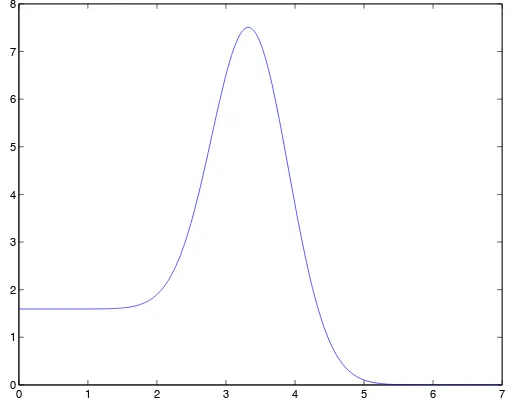
The fourth remark is about the optimal value of κ = κ∗. Figure 1 shows a typical shape for C_KG(t,κ), as a function of the parameterκ.

Our lower bound requires the maximization of C_KG(t,κ). In practice, the optimization can be

accelerated by using a one-dimensional FFT to bound the optimization interval and to guess the starting optimization value κstart. Therefore we adopt a two-step strategy which results in a

significant time saving:

Step 1 – Bounding the search domain We compute formula (8) via FFT and we obtain

C_KG(t,κ) on an equally spaced grid {κ1, . . . ,κM}. Then we perform a grid search to find

κm such that

κm= arg max_κ∈{κ1,...,κM}C G K(t,κ),

i.e. an estimate of the lower bound on such a grid. SinceC_KG(t,κm) is the best approximation we can get via FFT, we select κm as the starting point of the optimization routine in the second step. Extensive numerical tests show that the target function is unimodal, so the maximum ofC_KG(t,κ) should lie in the interval [κm−1,κm+1]. If the maximum is not unique

(i.e. it is achieved on two different points of the grid), we restrict the optimization to the interval delimited by these two values and we use their average as starting point.

Step 2 – Constrained optimization We perform an optimization for the integral in (8) to all

0 1 2 3 4 5 6 7

0 1 2 3 4 5 6 7 8

Figure 1. Lower boundCG_K(t,κ) as a function of the parameterκfor a mean reverting jump diffusion model. The

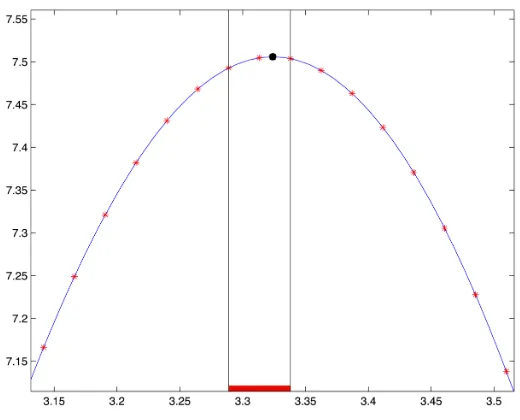
Figure 2. Optimization procedure for a mean reverting jump diffusion model. The basket is composed by four assets. Parameter values are as in Table 4 and strike priceK= 30. The blue line indicates the valuesCKG(t,κ) as a function

of the parameterκ. The red markers refer to values obtained via FFT. The black marker indicates the optimized

lower boundCKG = 7.5059. The search domain is restricted to the red segment. The true price estimated via Monte

Carlo simulation is 7.5768.

κ in the range [κm−1,κm+1]. We assume that the numerical quadrature is performed using

a grid with N integration points. Given the integration grid and a maturity T, we notice that all evaluations of the function ΨT in (9) do not depend on the variable κ over which

the optimization is performed. Hence it is possible to evaluate and store all instances of this function computed on the quadrature nodes and then use the stored values in the optimization.

Figure 2 shows the two-step procedure with reference to a mean reverting jump diffusion model. The lower bound can also be used for the computations of Greeks. The envelope theorem guaran-tees that changes in the optimizer of the objective do not contribute to the change in the objective function, see Takayama (1974) page 160. Therefore, assuming that interchange of differentiation and integration is allowed, the first-order sensitivity of the basket option price to a change in the spot price of a generic asset is given by

∂C_KG(t,κ∗) ∂Sk

=I

Z +∞

0

e−iγκ∗_Ψ

T(γ;δ)dγ≥0

e−δκ∗−r(T−t)1

π

Z +∞

0

e−iγκ∗∂ΨT(γ;δ)

∂Sk

dγ,

Similar formula can be computed for other Greeks.

Finally, the main point concerning formula (7) is that the approximated option price is always obtained through the optimization of a univariate Fourier inversion. The computational cost of the method isO(n2N+Mlog(M)), and increases quadratically with the number of assetsncomposing the basket. Therefore our technique does not suffer from the curse of dimensionality as it happens for many other Fourier inversion methods proposed in the literature (Hurd and Zhou (2010), Lord

Oosterlee (2008).

Looking at the remaining literature, the model free bounds of Hobsonet al.(2005b) and Laurence and Wang (2008) are the only bounds so general to cover all the models and the basket sizes we are interested in. Such model free bounds require one to compute prices of European call and put on each underlying and solve an optimization problem. However numerical experiments, available upon request, show that their performance in terms of computational speed and accuracy is very poor with respect to the pricing problem under examination.

Our method guarantees faster approximations. Basket options can be easily priced also for high dimensions, and a broader class of problems can be considered. Up to our knowledge, the only feasible alternative to our approximations is Monte Carlo simulation. However, using the bound

C_KG(t) as a control variate1, we can also improve the accuracy of a Monte Carlo method. Indeed, we rewrite Eq. (1) as

CK(t) =CKG(t) +e −r(T−t)

Et

(An(T)−K)+

−e−r(T−t)Et[(An(T)−K)I(G)]+.

We calculate C_KG(t) via formula (7) on the optimal approximating set G and we use Monte Carlo simulation to compute the two expected values, which are highly correlated. In this way the simula-tion error is considerably reduced. Our formula provides a ready-to-use control variate estimate that allows us to improve the accuracy of Monte Carlo simulations. The accuracy of our lower bound as well as our control variate are proved via extensive numerical tests on a battery of different models in section 5.

2. A fast bounded approximation through the arithmetic-geometric mean inequality

We discuss here new upper and lower bounds to the basket option price and we propose a price approximation lying between such bounds, exploiting the so-called geometric-arithmetic mean in-equality. This consists in a generalization of the Vorst (1992) approach to a characteristic function framework, allowing the basket weights to be negative.

DenotingJpos andJneg the sets of the indices corresponding to the positive and negative weights respectively, the basket can be rewritten as

An(T) =

X

k∈Jpos

wkSk(T)−

X

k∈Jneg

|wk|Sk(T) =cposAposn (T)−cnegAnegn (T), (10)

where

Apos_n (T) = P

k∈JposwkSk(T)

P

k∈Jposwk

, Aneg_n (T) = P

k∈Jneg|wk|Sk(T)

P

k∈Jneg|wk|

, (11)

and

cpos = X k∈Jpos

wk, cneg=

X

k∈Jneg

|wk|. (12)

We definewpos the vector having ask-th componentw_kpos=wk/Pk∈Jposwk, whenk∈Jpos and 0 whenk∈Jneg. Similarly, we definewneg the vector havingwneg_k =|wk|/P_k∈Jneg|wk|in thekth

position whenk∈Jneg and 0 whenk∈Jpos. We also define

Gpos_n (T) = Y k∈Jpos

Sk(T)w pos

k , Gneg

n (T) =

Y

k∈Jneg

Sk(T)w neg k ,

Ynpos(T) = lnGposn (T) and Ynneg(T) = lnGnegn (T).

AssumingK >01, we can now provide upper and lower bounds to the basket option price. We also obtain an approximation lying between such bounds, in this way generalizing Vorst (1992).

Proposition 2.1 A lower bound LAGK (t), an upper boundUKAG(t) and an approximation CKAG(t)

to the basket option value (1), such that LAG

K (t)≤CKAG(t)≈CK(t)≤UKAG(t), are obtained as

LAG_K (t) =e−r(T−t)Et[(cposGposn (T)−cnegGnegn (T)−K)+] +

cnege−r(T−t){_Et[G_nneg(T)]−_Et[Aneg_n (T)]}, (13)

U_KAG(t) =e−r(T−t)Et[(cposGposn (T)−cnegGnegn (T)−K)+] +

cpose−r(T−t){Et[Anpos(T)]−Et[Gposn (T)]}, (14)

C_KAG(t) =e−r(T−t)Et[(cposGnpos(T)−cnegGnegn (T)−K∗)+], (15)

where

K∗ =K−Et[cposAposn (T)] +Et[cposGposn (T)] +Et[cnegAnegn (T)]−Et[cnegGnegn (T)]. (16)

Proof:See Appendix B.

In the spirit of Vorst (1992), approximationC_KAG(t) replaces the random variablecposAposn (T)−

cneg_Aneg

n (T)−K with cposGposn (T)−cnegGnegn (T)−K∗ in the basket spread option payoff. Then the strike priceK∗ is corrected as in formula (16), so that the unbiasedness condition on the first moment is guaranteed.

We observe that pricing formulae (13), (14) and (15) depend on the value of a call option written on the difference betweencposGposn (T) and cnegGnegn (T), that is

e−r(T−t)Et[(cposGposn (T)−cnegGnegn (T)−K)+].

Therefore, we need the pricing of a spread option, that can be easily performed via the Hurd and Zhou (2010) method or through the approximation in Caldana and Fusai (2013), that we recall in Appendix C. These methods require the joint characteristic function of [ln(cposGposn (T)),ln(cnegGnegn (T))]|, that we state here for the sake of completeness:

Et[eln(iγ1c pos_Gpos

n (T))+iγ2ln(cnegGnegn (T))_{] =e}iγ1ln(cposGposn (t))+iγ2ln(cnegGnegn (t))_ϕ

T(γ1wpos+γ2wneg).

When the basket is strictly positive, Gn(T) = Gposn (T) and cpos = 1 by assumptions. We have then the following corollary:

Corollary 2.2 When the basket is strictly positive, a lower bound LAGK (t), an upper bound

U_KAG(t)and an approximationC_KAG(t)for the basket option value (1), such thatLAG_K (t)≤C_KAG(t)≈

1_{The strike priceK≤0 leads to}

CK(t)≤UKAG(t),are obtained as

LAG_K (t) =e−r(T−t)Et[(Gn(T)−K)+], (17)

U_KAG(t) =e−r(T−t)Et[(Gn(T)−K)+] +e−r(T−t){Et[An(T)]−Et[Gn(T)]}, (18)

C_KAG(t) =e−r(T−t)Et[(Gn(T)−K∗)+], (19)

where

K∗=K−_Et[An(T)] +Et[Gn(T)]. (20)

Proof:We consider Proposition (2.1) withGposn (T) =Gn(T), cpos= 1 and cneg = 0.

When weights are positive, pricing formulae (17),(18) and (19) require the pricing of a call option written onGn(T), rather than pricing a spread option. The call price is easily computed via Fourier inversion as

e−r(T−t)Et[(Gn(T)−K)+] =

e−δlnK−r(T−t) π

Z ∞

0

e−iγlnKΨG_T(γ;δ)dγ, (21)

where the characteristic functions ΨG_T of lnGn(T) is

ΨG_T(γ;δ) = ΦT(γ−i(δ+ 1),0,w, Yn(t))

δ2_+δ−γ2_{+ iγ(2δ+ 1)} , (22)

and the parameterδ tunes the damping factor.

Lower and upper bounds LAG_K (t) and U_KAG(t) in formulae (13), (14), (17) and (18) provide an interval for the approximation error ofC_KAG(t). Depending on the expected differences between the arithmetic and the geometric average, such an interval may be small or wide.

The main advantage of pricing based on the arithmetic-geometric mean inequality is its compu-tational speed. In the positive basket case, the computation of the bounded approximation requires one-dimensional integrations. The basket spread option case requires two-dimensional FFTs using the Hurd and Zhou (2010) method, or one-dimensional integrations using the approximation in Caldana and Fusai (2013). The computation ofLAG_K (t),C_KAG(t) andU_KAG(t) is very fast, regardless of the basket dimension. Its computational cost is linearly increasing in the number of assets, rather than quadratically as for the lower bound of section 1.

Proposition 2.1 and Corollary 2.2 provide very general bounded approximations, that can be computed when the model characteristic function is known. Numerical experiments in Section 5 show that the approximation CAG

K (t), based on the arithmetic-geometric mean inequality, is in general less accurate than the lower bound CK(t) discussed in Section 1. However the former is much faster than the latter and computing LAG_K (t), C_KAG(t) and U_KAG(t) may be very useful in all applications involving a large number of underlyings.

3. The geometric Brownian motion case

This section discusses in greater detail the geometric Brownian motion case and the explicit com-putation of the previously introduced price approximations.

We consider a multivariate Black–Scholes model. The dynamics are given by

wherer is the risk-free rate, q is the vector of dividend yields for each asset,1 is a vector whose entries are all equal to one, Σ is the covariance matrix, andWis ann-dimensional Brownian motion. The risk-neutral joint characteristic function of the n stock returns in the geometric Brownian motion case is

ϕT(γ) =eiγ

|_m(T−t)−1 2γ

|_Σγ(T−t)

, (24)

where

m=r1−q−1

2V ec(Σkk) (25)

and V ec(·) is the vectorization operator. From (6), the joint characteristic function of the log-returns and the log-geometric average is

ΦT(γ0,γ,w, Yn(t)) =eiγ0Yn(t)+i(γ

|_+γ

0w|)m(T−t)−1₂(γ|+γ0w|)Σ(γ+γ0w)(T−t)_{. (26)}

Expression (26) can be used to compute the proposed lower and upper bounds; however, in the geometric Brownian motion setting, all formulas can be explicitly computed, see details in Appendix D. The lower boundC_KG(t) given in formula (8) becomes

C_KG(t) = max

κ

e−r(T−t)

n

X

k=1

wkSk(t)e(r−qk)(T−t)N(ak

√

T −t−d)−KN(−d)

!+

(27)

where

d= κ−w

|_{(ln(S(t)) +m(T −t))}

σ∗√_T−t , ak=

Pn

j=1wjΣkj

σ∗ , σ

∗₌√_w|Σw

and we indicate withN(·) the standard Normal distribution function. The following value forκ is

a good starting point to implement the maximization in (27)

κstart=σ∗K −Pn

k=1wkSk(t)e(r−qk)(T−t)

Pn

k=1wkakSk(t)e(r−qk)(T−t) +

n

X

k=1 wk

lnSk(t) +

r−qk− Σkk

2

(T−t)

.

The expectationsEt[An(T)] andEt[Gn(T)] are

Et[An(T)] = n

X

k=1

wkSk(t)e(r−qk)(T−t) and Et[Gn(T)] =G(t)e

w|_m+σ∗2

2

(T−t) .

In the positive basket case, call option values involved in bounds through the arithmetic-geometric mean inequality can be obtained using a Black–Scholes formula. Indeed, each asset price Sk(T) is lognormally distributed. Since G(T) is a product of lognormally distributed variables, it is also lognormally distributed

G(T)∼ LN(ln(G(t)) +w|m(T −t), σ∗2(T −t))

and clearly alsoeXk(T) is lognormally distributed

Then, given a lognormal distributed random variableZ ∼ LN(ˆµ,σˆ2),

E[(Z−K)+] =eµˆ+ˆσ 2_/2

N

ˆ

µ−ln(K) + ˆσ2

ˆ

σ

−KN

ˆ

µ−ln(K) ˆ

σ

.

Trivial modifications occur to compute the bounded approximation for basket spread options, see Caldana and Fusai (2013).

4. Non-Gaussian price models

This section presents several price models on which we analyze the performance of our novel bounds. For each model, we give a brief description and we provide the risk-neutral joint characteristic function of asset log-returns ϕT(γ). The joint characteristic function of the log-returns and the log-geometric average ΦT (γ0,γ,w, Yn(t)) used in the bounds computation is then immediately obtained via formula (6).

4.1. A jump diffusion stock price model

Let us consider a generalization to an n-dimensional case of the two-dimensional jump diffusion process with asymmetric Laplace distributed jump size discussed in Huang and Kou (2006), with reference to the pricing of two dimensional barrier options in equity markets.

The components of the stock price vector, fork= 1, . . . , n, have the form

Sk(t) =Sk(0) exp

"

r−qk−

σ2_k

2 −λκk−λkκZk

t+σkWk(t) + Nk(t)

X

mZ=1

Zk(mZ) + N(t)

X

mY=1

Yk(mY)

#

, (28)

whereσk>0, fork= 1, . . . , n, and Wk, Wj are risk-neutral Brownian motions with instantaneous correlationρkj,|ρ|<1, fork, j = 1, . . . , n. In addition,

PNk(t)

mZ=1Zk(mZ), fork= 1, . . . , n, aren uni-variate compound Poisson processes driven by the Poisson processesNkwith intensity rateλk. This jump component is unique to each stock and describes the idiosyncratic shocks for that particular asset only. The idiosyncratic jump sizesZkare independently and identically distributed according to an asymmetric Laplace distribution AL(αkk, ξ_kk2 ). The model also allows for macroeconomic shocks described by

N(t)

X

mY=1

Y(mY) =





N(t)

X

mY=1

Y1(mY), . . . , N(t)

X

mY=1

Yn(mY)





|

,

which is an-dimensional compound Poisson process with intensity rate λ. Under the risk-neutral measureQthe jump sizesYare assumed to be independently and identically distributed according

to a multivariate asymmetric Laplace distributionMAL(α,ΣY), whereα= (α1, . . . , αn)| and ΣY

is ann×nmatrix whose elements are defined as

(ΣY)k,j=ξkξjρYkj, k, j = 1, . . . , n.

Finally, the quantitiesκk and κZk, k= 1, . . . , n, in (28) are, respectively,

κk=

Z

R2

[eyk−1]m_Q(dy) = Z

R

[eyk−1]m_Q(dyk) =

1 1−αk−ξ2_k/2

κZk =

Z

R

[ezk−1]m_Q(dzk) =

1

1−αkk−ξ_kk2 /2

−1.

Proposition 4.1 The joint characteristic function of the log-returns for the asymmetric Laplace

jump diffusion model is

ϕT(γ) = exp

h

(T−t)iγ|_η−1

2γ|Σγ+

λ

1−iγ|_α+γ|_ΣYγ/2 −λ+

Pn

k=1

λk

1−iγkαkk+γ2

kξ

2

kk/2

−λk

i

, (29)

where (Σ)k,j =σkσjρk,j andηk :=r−qk−σ2k/2−λκk−λkκZk, k= 1, . . . , n.

Proof:Straightforward generalization of Huang and Kou (2006) to the n-dimensional case.

4.2. Mean-reverting jump diffusion model

The third model is a mean-reverting jump diffusion that generalizes the model proposed by Hambly

et al. (2009) to describe the electricity spot price in energy markets. For k = 1, . . . , n, the spot price process Sk(t) is defined as the exponential of the sum of three components: a deterministic functionfk(t), a Gaussian Ornstein–Uhlenbeck process Xk(t), and a mean-reverting process with a jump componentYk(t):

Sk(t) = exp (fk(t) +Xk(t) +Yk(t)),

dXk=−αkXk(t)dt+σkdWk,

dYk =−αkYk(t−)dt+Jk+dN

+

k −J

−

kdN

− k .

The parameter σk is strictly positive and Wk is a risk-neutral Brownian motion. We assume a speed of mean reversionαk >0 for both the diffusion processXk(t) and the jump process Yk(t). The Brownian motions Wk and Wj have instantaneous correlation ρkj,|ρkj| < 1 for k 6= j and equal to 1 for k = j. We denote with N_k+ and N_k− Poisson processes with intensity λ+_k and λ−_k, respectively, and describe the positive and negative jump arrivals separately. The terms J_k+ and

J_k− are independent identically distributed random variables representing the jump size and we assume they are exponentially distributed with parameters 0< µ+_k <1 and µ−_k >0, respectively. We denote withη(T) the vector having elements

ηk(T) = (Xk(t) +Yk(t))(e−αk(T−t)−1) +fk(T)−fk(t)

and Σ(T) the matrix having elements

Σkj(T) =ρkj

σkσj

αk+αj

1−e−(αk+αj)(T−t)

.

Assuming independence between the jump processes we get the following result:

diffusion model is

ϕT(γ) = exp

"

iγ|η(T)−1

2γ

|_Σ(T)γ+

n

X

k=1 λ+_k αk

ln 1−iµ

+

kγke

−αk(T−t)

1−iµ+_kγk

!

+

n

X

k=1 λ−_k αk

ln 1 + iµ − kγke

−αk(T−t)

1 + iµ−_kγk

!#

Proof:Generalization of Hamblyet al. (2009) to then-dimensional case.

4.3. FX stochastic volatility model

To provide a coherent framework for the evaluation of FX basket options, we consider the model by De Colet al.(2013). The idea is to introduce a foreign exchange market featuring ncurrencies. De Colet al.(2013) start by considering the value of each of these currencies in units of an artificial currency that can be viewed as a universal num´eraire. The model is initially introduced under the risk neutral measure defined by the artificial currency. In this setting, S0,i(t) denotes the value at time tof one unit of the currency iin terms of the artificial currency. Each artificial exchange rate S0,i is modeled via a multi-variate stochastic volatility model with d independent square-root components, V(t) ∈ _Rd_{. According to De Col et al. (2013), the dimension d can be chosen} according to the specific problem. A further assumption is that the stochastic volatility components arecommon between the different S0,i. Formally, we write

dS0,i(t)

S0,i_(t) = (r

0_−ri_)dt−(ai₎>p

Diag(V(t))dZ(t), i= 1, . . . , n; (30)

dVk(t) =κk(θk−Vk(t))dt+ξk

p

Vk(t)dWk(t), k= 1, . . . , d; (31)

where κk, θk, ξk ∈ R are parameters in a square root dynamics. pDiag(V) denotes the diagonal

matrix with the square root of the elements of the vectorVin the main diagonal. In each monetary areai, the money-market account, based on the deterministic risk free rateri, satisfies the following ODE

dBi(t) =riBi(t)dt, i= 1, . . . , n.

Finally, De Col et al. (2013) assume an orthogonal correlation structure between the stochastic drivers

dhZk, Whi(t) =ρkδkhdt, k, h= 1, . . . , d, (32)

together withdhZk, Zhi(t) =δkhdt and dhWk, Whi(t) =δkhdt.

The philosophy behind this approach is that each exchange rate is driven by several independent noises Zk (k = 1, .., d), each with an independent stochastic variance factor Vk, to which Zk is partially correlated via ρk. The vectors ai (i= 1, . . . , n) describe how much each of the different volatilities contributes to the dynamics ofS0,i.

Following De Colet al.(2013), we now turn our attention to the exchange rateSi,j _{between two} different currencies, say iandj. We set by definitionSi,j =S0,j/S0,i.

The resulting dynamics ofSi,j = Si,j(t)

t≥0 under theQ

equal to

dSi,j(t) =Si,j(t)(ri−rj)dt+ (ai−aj)>pDiag(V(t))dZQi_{(t). (33)}

The valuation of vanilla FX options can be performed using standard Fourier based techniques, see De Colet al. (2013). In the sequel, we provide the characteristic function of the log-returns in order to approximate FX basket options.

Proposition4.3 The joint characteristic function of the log-returns in the model of De Col et al.

(2013) is given by

ϕT(γ) =eA(τ)+

Pd

k=1Bk(τ)Vk(t)_{, (34)}

where, forτ =T−twe have

A(τ) = n

X

j=1,j6=i

ri−rjiγjτ + d

X

k=1 κkθk

ξ2

k

(Qk−dk)τ −2 log

1−cke−dkτ 1−ck

,

Bk(τ) =

Qk−dk

ξ2

k

1−e−dkτ

1−cke−dkτ

,

dk=

q

Q2_k−4RkPk,

ck=

Qk−dk

Qk+dk

,

Pk= 1 2

n

X

j,l=1,j,l6=i

iγjiγlai_k−aj_k ai_k−al_k− 1

2 n

X

j=1,j6=i

ai_k−aj_k2iγj,

Qk=κk− n

X

j=1,j6=i

iγjBk(τ)

ai_k−aj_k

ρkξk,

Rk= 1 2ξ

2

k.

Proof. See De Colet al. (2013).

4.4. The WASC model

The Wishart Affine Stochastic Correlation (WASC) model, introduced by Da Fonsecaet al.(2007), is a model which is applicable to different asset classes whenever a realistic and analytically tractable description of instantaneous correlations among state variables is required see e.g. Escobar et al.

(2012). It describes ann-dimensional vector of assets (S1(t), . . . , Sn(t))>, t≥0 according to the following dynamics:

where Z(t) ∈ Rn is a vector Brownian motion and the returns’ covariance matrix Σ(t) evolves

according to the following matrix SDE:

dΣ(t) =

αQ>Q+MΣ(t) + Σ(t)M>

dt+pΣ(t)dW(t)Q+Q>dW(t)>pΣ(t), (36)

Σ(0)∈S_n+, (37)

where S_n+ denotes the cones of positive semidefinite matrices endowed with the scalar product given by the trace operator applied to the matrix product. In the dynamics above,M, Q∈GL(n) and we assume that M has negative eigenvalues, so as to ensure the stationarity of the process. Furthermore, we assumeα≥n−1, see Cuchieroet al. (2011).

The asymmetric correlation effects are modeled by introducing the following correlation structure among Brownian motions:

dZ(t) =p1−ρ>_{ρdB(t) +dW(t)ρ (38)}

whereρ∈_Rn_{, withρ∈[−1,1]}n _{and ρ}>_{ρ≤1. The model belongs to the class of multidimensional} stochastic volatility models. In the following, we follow the approach of Grasselli and Tebaldi (2008) and Da Fonsecaet al.(2007) and report their result on the joint Fourier transform of assets’ returns, that we adapt to our setting.

Proposition 4.4 Let τ :=T −t. Given a real vector γ ∈ Rn, the characteristic function of the WASC model is given by

ϕT(γ) = exp{A(τ) +T r[B(τ)Σ(t)]}

where

B(τ) =B22(τ)−1B21(τ),

B11(τ)B12(τ) B21(τ)B22(τ)

= expτ M+ iQ

>_{ρ γ}>

−2Q>Q

Λ − M+ iQ>ρ γ>>

!

,

Λ =−1

2 

(γ)

γ>+ i n

X

j=1

(γ)_jejj



,

A(τ) =−α

2

log(B22(τ)) +τM+ iQ>ργ>

>

+ iγ>1rτ,

where ejj denotes a matrix with a unique non zero entry along the main diagonal equal to one on

the positionjj.

Proof. See Da Fonsecaet al. (2007).

5. Numerical results

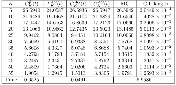
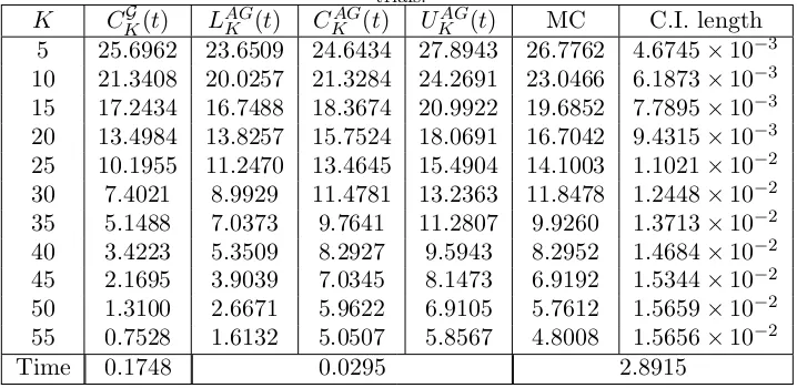
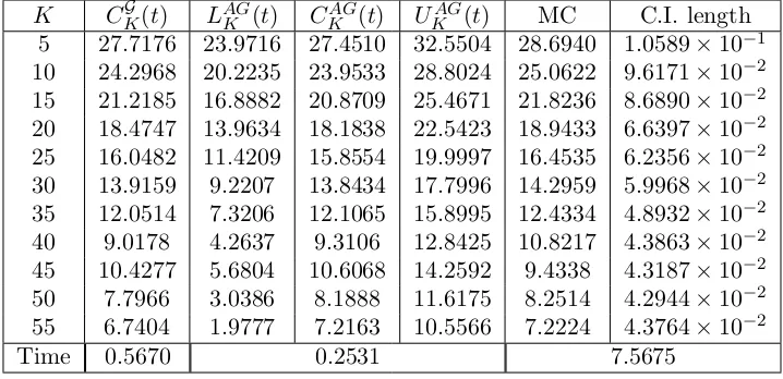
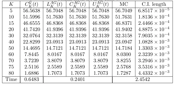
motion case and for each non-Gaussian model presented in Section 4. Numerical results are reported in Tables (2–11). Results for the positive basket case are given in Tables (2–6). Results for the basket spread option are in Tables (7–11).

At first we have to select a benchmark. To this aim we consider Monte Carlo simulation, using the lower boundC_KG(t) as a control variate, as described in Section 1. In this way the simulation error is considerably reduced. The Monte Carlo simulation for the geometric Brownian motion has been implemented by sampling from the lognormal distribution. For the jump diffusion model we sample from the Gaussian noise and the jump components. The other three models have been simulated through the Euler-Maruyama discretization scheme. The number of simulations is chosen depending on the model, as indicated in each table caption. Columns labeled with C.I. length give the length of the 95% mean-centered Monte Carlo confidence interval.

Table 1 compares the control variate (MC) and the crude (MCcr) Monte Carlo for each model. Model parameters are set as in Tables 2–6 and the option strike priceK is chosen to be close to at the money. The confidence interval length of each Monte Carlo simulation is also provided. Using the lower bound C_KG(t) as a control variate in the simulation, the standard error and therefore the confidence interval of the crude Monte Carlo estimate are significantly reduced. For example the length of the confidence interval in the geometric Brownian motion model is reduced from 8.2416×10−2 to 3.3707×10−3. A substantial reduction is also obtained for all other models. For example in the FX stochastic volatility model the confidence interval length is reduced from 1.2348×10−1 to 8.8989×10−4.

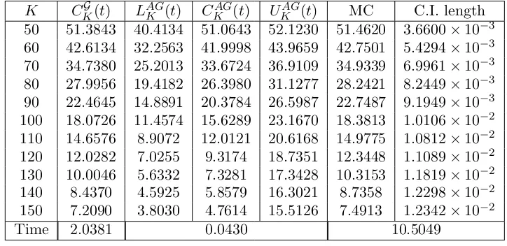
The bounds for the geometric Brownian motion in Table 2 and 7 are computed by exploiting the explicit formulas of section 3. For non-Gaussian models, integrals involved in all lower and upper bound computations are evaluated by means of a Gauss–Kronrod quadrature rule, using Matlab’s built-in functionquadgk. The optimization involved in the computation of C_KG(t) is performed via the Matlab functionfminuncfor the geometric Brownian motion and using fminbndin remaining cases. Spread options in formulae (13), (14) and (15) have been evaluated using formula (C2) in Appendix C. For all computations involving a Fourier inversion, we used a damping parameter

δ = 0.75. The bottom line of each table shows the average CPU time of a single option price evaluation. The quantity is measured in seconds and depends on the model and the pricing method. The best performances in terms of accuracy are generally obtained by the lower bound C_KG(t), that outperforms the approximation C_KAG(t) in most cases. The accuracy of the approximations depends on the basket distribution and is affected by the basket size and the presence of negative weights. In particular, the lower boundC_KG(t) is usually more accurate when the basket is small and weights are positive. Indeed, when the basket weights are strictly positive (Tables 2–6), the bound based on the approximating set argumentC_KG(t) always outperforms the arithmetic-geometric mean inequality approximation C_KAG(t). In the basket spread case (Tables 7–11), i.e. when weights can assume negative values, the lower bound C_KG(t) still provides good results but it is sometimes outperformed by the bounded approximationC_KAG(t). In particular, C_KAG(t) performs better than

C_KG(t) for out of the money options in Tables 7 and 6 and for in the money options in Table 8. In the pure spread option case in Table 10, the bounded approximation becomes exact and it is always more accurate thanC_KG(t).

Depending on expected differences between the arithmetic and the geometric average, the interval between lower and upper bounds [U_KAG(t)−LAG_K (t)] can be very small or very wide. For example, it is null in the spread option case of Table 10, providing an exact result. It is very large and practically useless for basket spread options in table 8. In general, the true price is closer toU_KAG(t) when the option is in the money, while it is closer toLAG_K (t) when the option is out of the money.

than the best methods they considered for a basket spread option (Borovkova et al. (2007) and Deelstraet al. (2010)).

The MRJD model, presented in Tables (4) and (6), is a nice example of the generality of our bounds. Other methods such as Hurd and Zhou (2010), Lord et al. (2008) and Jackson et al.

(2008) cannot cope with this model, because they require assumptions on the model characteristic function that rule out mean reverting models.

As an example of application, we tested two models calibrated to current market data. Results in Tables (5) and (10) refer to the stochastic volatility model for currencies of Section 4.3. We take the parameters from Table 1 in De Col et al. (2013), which features the result of a calibration performed on market data as of July 23rd 2010. Taking the perspective of a Japanese investor who seeks protections against fluctuations of both EUR-JPY and USD-JPY, we evaluate the payoff

w1SU SD,J P Y(T) +w2SEU R,J P Y(T)−K

+

.

Results in Table (6) refers to a two-asset basket option on FTSE and Eurostoxx 50 modeled with the WASC process of Section 4.4. The parameters refer to a calibration performed on August 20th 2008, as in Da Fonseca and Grasselli (2011).

The computational cost of our price approximation methods varies depending on the performed tests. Computations are extremely fast for the GBM, where no numerical integration is required and in addition we are able to choose a good starting point for the optimization problem. As the complexity of the model characteristic function increases, the computational cost increases as well. In Tables 3 and 8 we tested our methods by considering large baskets consisting of ten and twenty assets. The price approximation is always obtained at a reasonable time cost. Both methodologies involve the computation of one dimensional integrals, and hence they do not suffer from the curse of dimensionality, as opposed to the approach of Hurd and Zhou (2010), Lord

et al. (2008), Jackson et al. (2008) and Jaimungal and Surkov (2011). All these latter require an

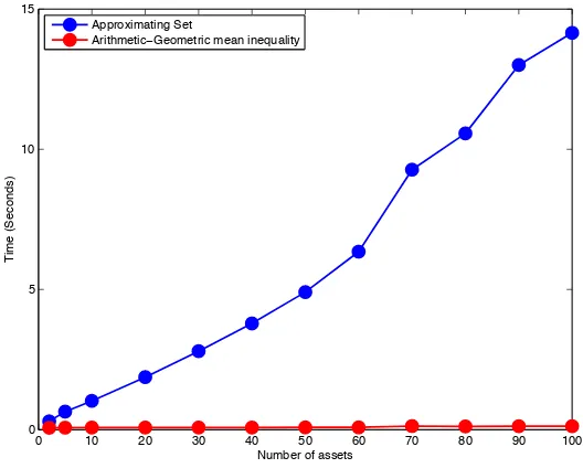
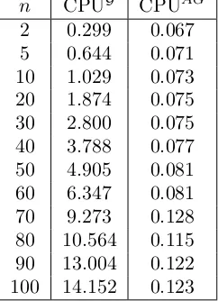
n-dimensional quadrature, and cannot be used in the practice when the basket dimension is high. Table 12 investigates the relation between CPU time and basket size, as we increase the number of assets up to 100. We select a basket with positive weights under the jump diffusion model of Section 4.1. We consider the two price approximations C_KG(t) and C_KAG(t) for an increasing basket size n. Column CPUG provides the CPU time for the lower bound in formula (7). CPU times for the approximation based on the arithmetic-geometric mean inequality of formula (19) are given in column CPUAG. The computation of the approximation C_KAG(t) is much faster than the lower bound C_KG(t) because its complexity is linear in the basket dimension and it does not require any optimization. This approximation can be very useful for pricing basket options written on an high number of underlying assets, in particular when the model characteristic function valuation is computationally expensive. On the other hand, the lower bound C_KG(t) is generally more accurate and it is also reasonably fast because its CPU time grows quadratically in the basket dimension. In our experiments, the price for a basket on 100 underlyings is computed in only 15.53 seconds. Considering basket spread options does not change the above considerations. Monte Carlo simulation in such a case turns out to be very slow and, given the same time budget of competing procedures, quite inaccurate. Numerical results are plotted in Figure 3.

6. Conclusions

Most methodologies in the basket option pricing literature are either restricted to a simple lognor-mal setting or to a model-dependent framework. In this paper we introduced novel methods which allow for a fast and reliable approximation of basket options, via lower and upper bounds. Such bounds rely on a rather weak assumption, i.e. the characteristic function of the vector of log-prices is known. This assumption is very general as most models which are commonly found in the literature allow for an explicit expression of this quantity either by means of the L´evy-Khintchine formula for L´evy processes or systems of (generalized) Riccati equations for affine processes. However, our approach is not restricted to those classes of models, provided the multivariate characteristic func-tion is known. We study the case of strictly positive basket weights as well as the negative one, i.e. the so-called basket spread option. We test our methodologies on different models: a Gaussian model, a jump diffusion model, a mean reverting jump diffusion model, a multi-factor stochastic volatility model with common factors among the underlyings and finally a stochastic correlation model. In particular we study two kinds of price approximations: an accurate lower bound based on an approximating set and a fast bounded approximation based on the arithmetic-geometric mean inequality. Both approximations are particularly appealing for higher dimensional problems, versus most existing methods in the literature that cannot be applied when the basket dimension is large, due to the significant computational cost. Moreover, by using one of our bounds as a control variate, we can largely improve the accuracy of the Monte Carlo estimate.

We believe that our solutions opens up the possibility of performing further investigations, for example in the study of the relationship between the implied volatility of a basket and its con-stituents, such as the S&P 500 index, and in portfolio selection applications.

References

Alexander, C. and Venkatramanan, A., Analytic approximations for multi-asset option pricing.Mathematical Finance, 2012,22, 667–689.

Beisser, J., Topics in finance—A conditional expectation approach to value Asian, basket and spread options. PhD thesis, Johannes Gutenberg University Mainz, 2001.

Bertsimas, D. and Popescu, I., On the relation between option and stock prices: A convex optimization approach.Operations research, 2002,50, 358–374.

Bjerksund, P. and Stensland, G., Closed form spread option valuation. Quantitative Finance, 2014, 14, 1785–1794.

Black, F. and Scholes, M., The pricing of option and corporate liabilities. Journal of Political Economy, 1973,81, 637–654.

Borovkova, S., Permana, F.J. and Weide, H., A closed-form approach to the valuation and hedging of basket and spread options.Journal of Derivatives, 2007,14, 8–24.

Caldana, R. and Fusai, G., A general closed-form spread option pricing formula. Journal of Banking & Finance, 2013,37, 4893—4906.

Carmona, R. and Durrelman, V., Pricing and Hedging Spread Options.SIAM Review, 2003,45.

Carr, P. and Madan, D., Option valuation using the fast Fourier transform. Journal of Computational Finance, 2000,2, 61–73.

Cuchiero, C., Filipovi´c, D., Mayerhofer, E. and Teichmann, J., Affine Processes on Positive Semidefinite Matrices. Annals of Applied Probability, 2011,21, 397–463.

Curran, M., Valuing Asian and portfolio options by conditioning on the geometric mean price.Managment Science, 1994, 40, 1705–1711.

Da Fonseca, J. and Grasselli, M., Riding on the smiles.Quantitative Finance, 2011,11, 1609–1632. Da Fonseca, J., Grasselli, M. and Tebaldi, C., Option pricing when correlations are stochastic: an analytical

framework.Review of Derivatives Research, 2007, 10, 151–180.

D’Aspremont, A. and El Ghaoui, L., Static arbitrage bounds on basket option prices. Mathematical Pro-gramming, 2006,106, 467–489.

Journal of Banking & Finance, 2013,37, 3799–3818.

Deelstra, G., Diallo, I. and Vanmaele, M., Bounds for Asian basket options.Journal of Computational and Applied Mathematics, 2008,218, 215–228.

Deelstra, G., Liinev, J. and Vanmaele, M., Pricing of arithmetic basket options by conditioning.Insurance: Mathematics and Economics, 2004,31, 55–77.

Deelstra, G., Petkovic, A. and M.Vanmaele, Pricing and hedging Asian basket spread options.Journal of Computational and Applied Mathematics, 2010, 234, 2814–2830.

Dhaene, J., Denuit, M., Goovaerts, M.J., Kaas, R. and Vyncke, D., The concept of comonotonicity in actuarial science and finance: applications.. Insurance: Mathematics and Economics, 2002a, 31, 133– 161.

Dhaene, J., Denuit, M., Goovaerts, M.J., Kaas, R. and Vyncke, D., The concept of comonotonicity in actuarial science and finance: Theory..Insurance: Mathematics and Economics, 2002b, 31, 3–33. Escobar, M., Arian, H. and Seco, L., CreditGrades Framework within Stochastic Covariance Models.Journal

of Mathematical Finance, 2012,4, 303—314.

Flamouris, D. and Giamouridis, D., Approximate basket option valuation for a simplified jump process. Journal of Futures Markets, 2007,27, 819– 837.

Gentle, D., Basket weaving.Risk, 1993,6, 51–52.

Glasserman, P.,Monte Carlo Methods in Financial Engineering, Stochastic Modelling and Applied Proba-bility Vol. 53, , 2003, Springer.

Grasselli, M. and Tebaldi, C., Solvable Affine Term Structure Models. Mathematical Finance, 2008, 18, 135–153.

Hambly, B., Howison, S. and Kluge, T., Modelling spikes and pricing swing options in electricity markets. Quantitative Finance, 2009, 9, 937–949.

Hobson, D., Laurence, P. and Wang, T., Static-arbitrage optimal sub-replicating strategies for basket options. Insurance: Mathematics and Economics, 2005a,37, 553–572.

Hobson, D., Laurence, P. and Wang, T., Static-arbitrage upper bounds for the price of basket options. Quantitative Finance, 2005b, 5.

Huang, Z. and Kou, S., First passage times and analytical solutions for options on two assets with jump risk [online]. , 2006. (accessed ????).

Hurd, T.R. and Zhou, Z., A Fourier transform method for spread option pricing.SIAM Journal of Financial Mathematics, 2010,1, 142–157.

Huynh, C.B., Back to Baskets.Risk, 1993,7, 59–61.

Jackson, K.R., Jaimungal, S. and Surkov, V., Fourier space time-stepping for option pricing with L´evy models. The Journal of Computational Finance, 2008,12, 1–29.

Jaimungal, S. and Surkov, V., L´evy Based Cross-Commodity Models and Derivative Valuation.SIAM Jour-nal of Financial Mathematics, 2011,2, 464–487.

Johnson, N.L., Systems of Frequency Curves Generated by Methods of Translation.Biometrika, 1949,36, 149–176.

Ju, E., Pricing Asian and basket options via Taylor expansion.Journal of Computational Finance, 2002,5, 79–103.

Krekel, M., Kock, J.D., Korn, R. and Man, T., An Analysis of Pricing Methods for Baskets Options.Wilmott, 2004,3, 82–89.

Laurence, P. and Wang, T., What’s a basket worth?.Risk, 2004, pp. 73–77.

Laurence, P. and Wang, T., Sharp upper and lower bounds for basket options.Applied Mathematical Finance, 2005,12, 253–282.

Laurence, P. and Wang, T., Distribution-free upper bounds for spread options and market-implied anti-monotonicity gap.The European Journal of Finance, 2008,14, 717–734.

Lee, R., Option pricing by transform methods: extensions, unification and error control.Journal of Compu-tational Finance, 2004,7, 51—86.

Leentvaar, C.C.W. and Oosterlee, C.W., Multi-asset option pricing using a parallel Fourier-based technique. The Journal of Computational Finance, 2008, 12, 1–26.

Levy, E., Pricing European average rate currency options.. Journal of International Money and Finance, 1992,11, 474–491.

Lewis, A.,Option valuation under stochastic volatility, 2000, Finance Press.

Lord, R., Partially exact and bounded approximations for arithmetic Asian options.Journal of Computa-tional Finance, 2006,10, 1–52.

Lord, R., Fang, F., Bervoets, F. and Oosterlee, C.W., A fast and accurate FFT-based method for pricing early-exercise options under L´evy processes.SIAM J. Scientific Computing, 2008,30, 1678–1705. Milevsky, M.A. and Posner, S.E., A Closed-Form Approximation for Valuing Basket Options. Journal of

Derivatives, 1998a,5, 54–61.

Milevsky, M.A. and Posner, S.E., Valuing exotic options by approximating the SPD with higher moments. Journal of Financial Engineering, 1998b,7, 109–125.

Nielsen, J.A. and Sandmann, K., Pricing bounds on Asian options.Journal of Financial and Quantitative Analysis, 2003,38, 449–473.

Rogers, L.C.G. and Shi, Z., The value of an Asian option.Journal of Applied Probability, 1995,32, 1077– 1088.

Takayama, A.,Mathematical Economics, 1974, The Dryden Press.

Thompson, G.W.P., Topics in mathematical finance. PhD thesis, University of Cambridge, 1999.

Vanmaele, M., Deelstra, G. and Liinev, G., Approximation of stop-loss premiums involving sums of lognor-mals by conditioning on two variables. Insurance: Mathematics and Economics, 2004, 35, 343–367. Vorst, T., Prices and Hedge Ratios of Average Exchange Rate Options.International Review of Financial

Analysis, 1992,1, 179–193.

Vyncke, D., Goovaerts, M.J. and Dhaene, J., An accurate analytical approximation for the price of a European-style arithmetic Asian option.Finance, 2004,25, 121–139.

Xu, G. and Zheng, H., Approximate basket options valuation for a jump-diffusion model.Insurance: Math-ematics and Economics, 2009,45, 188–194.

Xu, G. and Zheng, H., Basket options valuation for a local volatility jump-diffusion model with the asymp-totic expansion method.Insurance: Mathematics and Economics, 2010,47, 415–422.

Xu, G. and Zheng, H., Lower Bound Approximation to Basket Option Values for Local Volatility Jump-Diffusion Models.International Journal of Theoretical and Applied Finance, 2014, 17.

Zhou, J. and Wang, X., Accurate closed-form approximation for pricing Asian and basket options.Applied Stochastic Models in Business and Industry, 2008,24, 343–358.

Appendix A: Proof of Proposition 1.1

We denote by f(Xk, Yn) the joint bivariate probability density of Xk(T) and the log-geometric averageYn(T). We consider the lower bound to the basket option payoff in T, as in formula (4):

Et[(An(T)−K)I(G)],

where G = {ω : Yn(T) > κ}. We introduce the damping factor exp(δκ) according to Carr and

Madan (2000) and compute the Fourier transform with respect toκ. We obtain

ΨT(γ;δ) =

Z

R

eiγκ+δκ

Et[(An(T)−K)I(G)]dκ

= Z

R

eiγκ+δκ

"

Et

" _n

X

k=1

wkSk(T)−K

!

I(G) ##

dκ

= Z

R

eiγκ+δκ

" _n X

k=1

wkEt[Sk(T)I(G)]

#

dκ−

Z

R

eiγκ+δκ

Et[KI(G)]dκ

So the first part becomes:

Ψ1_T(γ;δ) = Z

R

eiγκ+δκ

" _n X

k=1

wkEt[Sk(T)I(G)]

#

dκ

= Z

R

eiγκ+δκ

" _n X k=1 wk Z R

Z +∞

κ

Sk(t)eXk(T)f(Xk, Yn)dXkdYn

# dκ = n X k=1 wk Z R Z R Z Yn −∞

eiγκ+δκ_d

κ

Sk(t)eXk(T)f(Xk, Yn)dXkdYn

= 1

iγ+δ

n X k=1 wk Z R Z R

ei(γ−iδ)Yn(T)Sk(t)eXk(T)f(Xk, Yn)dXkdYn

= 1

iγ+δ

n

X

k=1

wkSk(t)Et

h

ei(γ−iδ)Yn(T)+Xk(T)i

= 1

iγ+δ

n

X

k=1

wkSk(t) ΦT (γ−iδ,−iek,w, Yn(t)).

The second part becomes:

Ψ2_T(γ;δ) = Z

R

eiγκ+δκ

Et[KI(G)]dκ

= Z

R

eiγκ+δκ

Z

R

Z +∞

κ

Kf(Xk, Yn)dXkdYn

dκ = Z R Z R Z Yn −∞

eiγκ+δκ_dκ

Kf(Xk, Yn)dXkdYn

= 1

iγ+δ

Z

R

Z

R

ei(γ−iδ)Yn(T)Kf(Xk, Yn)dXkdYn

= 1

iγ+δKEt

h

ei(γ−iδ)Yn(T)i

= 1

iγ+δKΦT(γ−iδ,0,w, Yn(t)).

Remembering the damping factor, we read the Fourier inversion as

e−δκ

π

Z +∞

0

e−iγκ_{Ψ(γ;δ)dγ.}

Formula (8) is obtained by discounting, taking the positive part and maximizing with respect to

κ. The moment condition {ek, δw+ek} ∈ AX, ∀k = 1,· · · , n, can be easily deduced from (Lee

Appendix B: Proof of Proposition 2.1

Due to the arithmetic-geometric mean inequality, Aposn (T) ≥ Gposn (T), and Anegn (T) ≥ Gnegn (T). Through the put-call parity we have

(cposAposn (T)−cnegAnegn (T)−K)+≥(cposGposn (T)−cnegAnegn (T)−K)+= (cnegAnegn (T) +K−cposGposn (T))++cposGposn (T)−cnegAnegn (T)−K ≥ (cneg_Gneg

n (T) +K−cposGposn (T))++cposGposn (T)−cnegAnegn (T)−K= (cposGposn (T)−cnegGnegn (T)−K)++cnegGnegn (T)−cnegAnegn (T),

and

(cposAposn (T)−cnegAnegn (T)−K)+≤(cposAposn (T)−cnegGnegn (T)−K)+= (cnegGnegn (T) +K−cposAposn (T))++cposAposn (T)−cnegGnegn (T)−K ≤ (cnegGnegn (T) +K−cposGposn (T))++cposAposn (T)−cnegGnegn (T)−K=

(cposGposn (T)−cnegGnegn (T)−K)++cposAposn (T)−cposGposn (T).

The proof ends taking the expectation of above inequalities and discounting.

Appendix C: Spread option approximation

We recall here the spread option pricing formula proposed in Caldana and Fusai (2013). LetS1(t)

andS2(t) be two stock price processes. The time 0 no-arbitrage fair price of a spread option is

SpreadK(0) =e−rTE(S1(T)−S2(T)−K)+, (C1)

Let u = (u1, u2)| ∈ R2 and X(t) = (lnS1(t),lnS2(t))| and consider the joint characteristic

function

ΦT(u) = ΦT(u1, u2) =E

h

eiu1lnS1(T)+iu2lnS2(T)

i =E

h

eiu|X(T)

i

.

Proposition C.1 The approximate spread option value CKk,α(0) is given in terms of a Fourier

inversion formula as

Spreadk,α_K (0) =

e−δk−rT π

Z +∞

0

e−iγkΨT(γ;δ, α)dγ

+

, (C2)

where

ΨT(γ;δ, α) =

ei(γ−iδ) ln(ΦT(0,−iα))

i(γ−iδ) [ΦT((γ−iδ)−i,−α(γ−iδ))−

and

α= F2(0, T)

F2(0, T) +K

, (C4)

k= ln F2(0, T) +K. (C5)

The quantityF2(0, T) =E[S2(T)] in formulas (C4) and (C5) is the forward price of the second

asset at time 0 for delivery at future date T. Using the characteristic function properties, we can write F2(0, T) = ΦT(0,−i). The parameter δ tunes an exponentially decaying term introduced to allow the integration in the Fourier space.

Appendix D: Proofs for the geometric Brownian motion case

Let us introduce the notation

ln(S(t)) = 

 

logS1(t)

.. . logSn(t)





.

We consider the set

G={ω :Yn(T)>κ}

=

ω :w|

ln(S(t)) +

r1−q−1

2V ec(Σkk)

(T −t) +√ΣW(T−t)

>κ

.

We see thatw|√ΣW(T−t) has the same distribution as a univariate Brownian motionσ∗W∗(T− t), whereσ∗ =√w|_{Σw. Considering mas in formula (25), we can write the setG as}

G=

ω :Z > d= κ−w

|_{(ln(S(t)) +m(T −t))}

σ∗√T−t

,

whereZ is a standard Normal random variable. We can write the expectation in (4) as

Et[(An(T)−K)I(G)]+=Et[Et[An(T)−K|G]I(G)]+ =Et[Et[An(T)−K|Z]I(Z > d)]+.

Conditionally to the random variableZ, the vector √ΣW(T−t) is distributed like a multivariate Normal with meanµand varianceV, with their elements defined for k, j = 1, . . . , n as

µk=Zak

√

T−t, Vkj = (T −t)(Σkj−akaj), ak =

Pn

j=1wjΣkj

σ∗ ,

and we indicate with Σkj the element of Σ in position (k, j). Due to this fact, S(T)|Z follows a multivariate lognormalMLN( ˆµ,Vˆ), where, fork, j = 1, . . . , n,

ˆ

µk = lnSk(t) + (r−qk−Σkk/2)(T −t) +Zak

√ T−t,

ˆ