Nonlinear oscillatory rarefied gas flow inside a rectangular cavity
Peng Wang,1Lianhua Zhu,1,2Wei Su,1Lei Wu,1and Yonghao Zhang1,*
1James Weir Fluids Laboratory, Department of Mechanical and Aerospace Engineering, University of Strathclyde,
Glasgow G1 1XJ, United Kingdom
2State Key Laboratory of Coal Combustion, Huazhong University of Science and Technology, Wuhan 430074, China
(Received 1 February 2018; published 5 April 2018)
The nonlinear oscillation of rarefied gas flow inside a two-dimensional rectangular cavity is investigated on the basis of the Shakhov kinetic equation. The gas dynamics, heat transfer, and damping force are studied numerically via the discrete unified gas-kinetic scheme for a wide range of parameters, including gas rarefaction, cavity aspect ratio, and oscillation frequency. Contrary to the linear oscillation where the velocity, temperature, and heat flux are symmetrical and oscillate with the same frequency as the oscillating lid, flow properties in nonlinear oscillatory cases turn out to be asymmetrical, and second-harmonic oscillation of the temperature field is observed. As a consequence, the amplitude of the shear stress near the top-right corner of the cavity could be several times larger than that at the top-left corner, while the temperature at the top-right corner could be significantly higher than the wall temperature in nearly the whole oscillation period. For the linear oscillation with the frequency over a critical value, and for the nonlinear oscillation, the heat transfer from the hot to cold region dominates inside the cavity, which is contrary to the anti-Fourier heat transfer in a low-speed rarefied lid-driven cavity flow. The damping force exerted on the oscillating lid is studied in detail, and the scaling laws are developed to describe the dependency of the resonance and antiresonance frequencies (corresponding to the damping force at a local maximum and minimum, respectively) on the reciprocal aspect ratio from the near hydrodynamic to highly rarefied regimes. These findings could be useful in the design of the micro-electro-mechanical devices operating in the nonlinear-flow regime.
DOI:10.1103/PhysRevE.97.043103
I. INTRODUCTION
Oscillatory gas motion at the micro- and nanoscale has attracted significant attention due to the development of electro-mechanical systems (MEMS) including the micro-accelerometer, inertial sensor, and actuators [1]. Since the surface-area-to-volume ratio in MEMS devices is large, sur-face forces such as the damping exerted on the oscillating parts by the gas are important for the design of moving microdevices [2].
To understand and quantify the damping, the gas rarefaction effect, caused by the small characteristic length scale of the MEMS, should be taken into account. The degree of gas rarefaction is normally categorized by the Knudsen number (Kn), which is defined as the ratio of the mean free path of gas molecules to the characteristic flow length. Most MEMS devices operate in the slip (10−3Kn0.1) and early tran-sition regimes (0.1Kn1) [3,4], where the Navier–Stokes equations fail, and the kinetic theory approach should be adopted in study of rarefied gas dynamics [5,6].
To date, gas damping has been investigated by seeking solutions of gas kinetic equations through the direct simulation Monte Carlo (DSMC) method [3,7–12] and the discrete ve-locity method (DVM) [4,5,13–17]. Some analytical solutions have also been obtained for simple one-dimensional (1D) and
two-dimensional (2D) oscillatory flows in the slip and free molecular (Kn10) flow regimes [3,13,17–19].
In general, the DSMC and DVM are robust approaches for the simulation of rarefied gas flows in respectively high-speed and low-speed flow regimes. However, most of the aforemen-tioned studies were focused on the oscillatory gas flows in the transition regime (0.1Kn10) [5,7,9,10,15,18,20,21]. This is mainly due to the well-known intrinsic limitation that the computational time step and spatial mesh size in these two methods should be smaller than the mean collision time and the mean free path of gas molecules, respectively, resulting in an extremely expensive computations in the near hydrodynamic regime, i.e., Kn0.1. Special slip boundary treatments were introduced to improve the predictive capability in studying the oscillatory rarefied flow in the slip and early transition regimes [3,13,22]. However, these methods can only capture some of the bulk properties [12].
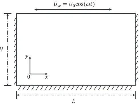
FIG. 1. Schematic diagram of the oscillatory flow in a rectangular cavity. The coordinate origin is located at the bottom-left corner of the cavity.
flow can be regarded as a linear system. However, the nonlin-ear oscillation may be possible; for example, the oscillation frequency of MEMS device could reach 110 GHz, and the oscillation amplitude could reach several nanometers, so that the oscillation speed could be 330 m/s which is comparable or even larger than the sonic speed [16,25–28]. The nonlinear oscillation may dramatically change the flow behavior and damping. Besides, high oscillatory frequency could further ag-gravate the degree of rarefaction [25]. Therefore, to accurately predict the gas damping in nonlinear oscillatory microsystems, the nonlinearity and compressibility of the flow should be taken into account.
In fact, Tsuji [16]et al.and Aokiet al.[27] recently applied the Boltzmann model equation to study the nonlinear motion of a rarefied gas caused by a plate oscillating in its normal direc-tion (1D problem). As far as the authors are aware of, however, direct investigation of the nonlinear oscillation in lid-driven cavity flows from the hydrodynamic to free molecular regimes is absent. Little effort has been devoted to understanding the heat transfer in nonlinear rarefied oscillatory flow, which plays a significant role in MEMS devices [16,27,29,30].
This work is devoted to studying the nonlinear oscillatory rarefied gas flow in a 2D rectangular cavity on the basis of the gas kinetic equation. We introduce the Shakhov model in Sec.II and the numerical scheme in Sec.III. Numerical results of the gas dynamics, heat transfer, and damping force in both linear and nonlinear oscillations over a wide range of gas rarefaction, cavity aspect ratio, and oscillation frequency are presented, compared, and discussed in Sec.IV, which is followed by the conclusions in Sec.V.
II. PROBLEM FORMULATION
We consider a rarefied gas flow in a 2D rectangular cavity driven by a lid aty =H. The lid oscillates harmonically in the
xdirection with a frequencyω, see Fig.1. The velocity of the oscillating lid is given by
Uw=U0cos(ωt), (1)
where U0 is the amplitude of the oscillating velocity, and
t is the time. The other three walls at x=0, x =L, and
y =0 are fixed, and all four walls are isothermal with a fixed temperatureTw.
The problem considered is characterized by the aspect ratio of the cavityA, the Mach number Ma, the Strouhal number St, and the Knudsen number Kn, which are, respectively, defined by
A= L
H, Ma=
U0 √
γ RTw
, St= ωH
vm
, Kn= λ
H, (2)
where γ is the specific-heat ratio,vm= √
2RTw is the most probable molecular velocity with R being the specific gas constant, andλis the mean free path of gas molecules, which is related to the shear viscosityμof the gas as
λ= μ(T =Tw) p
π RTw
2 . (3)
wherep=ρRTwis the pressure andρis the density. In this work, the hard-sphere molecular model is used, where the shear viscosity of the gas is determined by the gas temperature in the following way:
μ=μ(T =Tw)
T
Tw
0.5
. (4)
The gas kinetic theory is used to investigate how the flow responds to variations of the Knudsen number, the Strouhal number, the Mach number, and the aspect ratio of the cavity. To this end, the Shakhov equation is adopted, which has been widely used to describe the dynamics of monotonic gases [31]. In the absence of external force, it takes the form of
∂f
∂t +ξ·∇f = −
1
τ[f −f S
], (5)
where f(x,ξ,t) is the velocity distribution function of gas molecules at the position x=(x,y,z) and time t, withξ = (ξx,ξy,ξz) being the molecular velocity. fS is the reference distribution function expressed by the Maxwellian distribution functionfeq and a heat flux correction term:
fS=feq
1+(1−Pr) c·q 5pRT
c2
RT −5)
, (6)
where c=ξ−U is the peculiar velocity with U being the macroscopic flow velocity,q =12 cc2f dξ is the heat flux, andT is the temperature of the gas. The collision timeτ in Eq. (5) is related to the viscosityμand the pressurep=ρRT
by τ =μ/p. The Maxwellian distribution function feq is given by
feq = ρ
(2π RT)3/2 exp
− c2 2RT
. (7)
The conservative variables W ≡(ρ,ρU,ρE)T are calcu-lated from the velocity moments of the velocity distribution function:
W =
ψf dξ, (8)
Since only the 2D problem is considered in this work, two reduced velocity distribution functions are introduced to cast the three-dimensional molecular velocity space into 2D space [32]:
g=
f(x,ξ,t)dξz, h=
ξz2f(x,ξ,t)dξz. (9)
For convenience, in what follows we denote ξ =(ξx,ξy) andx =(x,y). The governing equations for the two reduced distribution functions can be deduced from Eq. (5) as
∂g
∂t +ξ ·∇g=g = −
1
τ[g−g
S], (10a)
∂h
∂t +ξ ·∇h=h= −
1
τ[h−h S
], (10b)
where the reduced reference distribution functions aregS= geq+g
PrandhS=heq+hPr, with
geq = ρ
2π RT exp
− c2 2RT
, (11a)
heq =RT geq, (11b)
gPr =(1−Pr) c·q 5pRT
c2
RT −4
geq, (11c)
hPr =(1−Pr) c·q 5pRT
c2
RT −2
heq. (11d)
It is clear that the governing equations forgandhin Eq. (10) can be expressed in the following compact form:
∂φ
∂t +ξ·∇φ== −
1
τ[φ−φ S
], (12)
where the symbolφis used to representgorh.
III. NUMERICAL METHOD
The discrete unified gas-kinetic scheme (DUGKS) is used to solve the Shakhov equation [33,34], which is essentially an explicit finite-volume method. With the intrinsic coupling of molecular collision and transport processes in determining of the flux across the cell interface, the computational time step and mesh size are not limited by the mean collision time and mean free path of gas molecules, respectively, so that the multiscale-flow physics can be efficiently and self-adaptively captured from the hydrodynamic to the free-molecular-flow regimes. In addition, DUGKS has second-order accuracy in both temporal and spatial discretizations. The capacity of DUGKS has been evaluated for gas flows by comparing with the lattice Boltzmann method [35–38], the spectral method [38,39], the DVM [40], and the DSMC [41,42]. It has also been successfully applied to study the phonon transport [43], turbulent flows [38,39,44], and thermally induced nonequilib-rium flows [42].
To solve Eq. (12), the computational domain is first divided into control cells (the trapezoidal cells are applied in this study). By integrating Eq. (12) in a cellVj (centered atxj) from time tn to tn+1, and by using the midpoint rule for the temporal integration of the convection term and the trapezoidal rule for the collision term, one obtains the following evolution
equation [33]:
˜
φjn+1=φ˜j+,n− t
|Vj| Fn+1/2
j , (13)
wheret =tn+1−tn, and
Fn+1/2
j =
∂Vj
(ξ·n)φ(x,ξ,tn+1/2)dS, (14)
is the flux across the cell interface, |Vj| and ∂Vj are the volume and surface of cellVj,n is the outward unit vector normal to cell interface, and φjn=V
jφ(x,ξ,tn)dx/|Vj| is the cell average of the distribution function. We have also introduced two auxiliary functions: ˜φ=φ−(t /2) and
˜
φ+=φ+(t /2).
Since the mass, momentum, and energy are conserved during the collision, macroscopic variables can be calculated from
ρ=
˜
gdξ, ρU =
ξgd˜ ξ, ρE=1
2
(ξ2g˜+h˜)dξ,
(15) and the heat flux from
q = 2τ
2τ+tPrq˜, with ˜q= 1 2
c(c2g˜+h˜)dξ. (16)
In practical computations, the evolution of ˜φ is tracked according to Eq. (13), instead of the original distribution functionsφ, to avoid the implicit computations.
The key procedure in updating ˜φis to evaluate the fluxFin Eq. (14), which is solely determined by the gas distribution function φn+1/2(xf,ξ). To do so, in DUGKS, Eq. (12) is integrated along the characteristic line within a half time step
s=t /2 [33],
φn+1/2(xf,ξ)−φn(xf −ξs,ξ)
= s 2
n
(xf−ξs,ξ)+ s
2 n+1/2(x
f,ξ), (17)
where time integration of the collision term is approximated by the trapezoidal rule. Again, to remove the implicitness in Eq. (17), we introduce two other distribution functions:
¯
φ=φ−s
2, φ¯
+=φ+s
2. (18)
Then Eq. (17) is expressed explicitly as
¯
φn+1/2(xf,ξ)=φ¯+,n(xf−ξs,ξ). (19)
Therefore, once ¯φ+,n(x
f−ξs,ξ) is obtained, the distribu-tion funcdistribu-tion ¯φn+1/2(x
f,ξ) can be determined from Eq. (19). Note that the conservative variables and heat flux can also be evaluated from ¯φas
ρ=
¯
gdξ, ρu=
ξgd¯ ξ, ρE= 1
2
(ξ2g¯+h¯)dξ,
(20)
and
q = 2τ
2τ+sPrq¯, with ¯q= 1 2
c(c2g¯+h¯)dξ, (21)
distribution function across the cell interface can be calculated from Eq. (18):
φn+1/2(xf,ξ)= 2τ
2τ +sφ¯ n+1/2(x
f,ξ)
+ s
2τ +sφ
S,n+1/2(x
f,ξ). (22)
In this work, ¯φ+,n(xf−ξs,ξ) is constructed as
¯
φ+,n(xf−ξs,ξ)=φ¯+,n(xj,ξ)+(xf−xj −ξs)·σj,
(xf −ξs) ∈ Vj, (23)
whereσj is the slope of ¯φ+in the cellj, which is computed by the central difference method. Note that σj can also be approximated by some gradient limiters for problems with discontinuities [41]. The flux can then be computed from Eq. (22). Finally, ˜φat the cell center can be updated according to Eq. (13).
In numerical simulations, the continuous molecular velocity space is discretized into a finite discrete velocity set{ξi}[32]. Distribution functions such as ˜gand ˜hare defined at a number of discrete velocity points as ˜gi and ˜hi. Then, the appropriate quadrature rule is adopted to calculate the moments: ρ = iig˜i,ρU= iiξig˜i, and ρE= 12 ii(ξi2g˜i+h˜i), wherei is the weight for the corresponding quadrature rule. Note that the time step of explicit time marching in the DUGKS is solely determined by the Courant–Friedrichs–Lewy (CFL) condition, i.e.,t =ηxmin/ξmax, whereηis the CFL number,
xminis the minimum grid spacing, andξmaxis the maximum discrete velocity.
IV. RESULTS AND DISCUSSION
The numerical simulations are performed covering a wide range of rarefaction: Kn=10, 1, 0.1, 0.01, and 0.001. Two Mach numbers, i.e., Ma=0.01 and 1.2, are chosen to represent the linear and nonlinear oscillations, respectively. Various aspect ratios and Strouhal numbers are considered.
In the simulation, all the cavity walls are assumed to be fully diffuse; that is, the velocity distribution of the reflected gas molecules at the walls is Maxwellian with the wall temperature and velocity:
¯
φ(xw,ξi,tn+s)=φeq(ξi;ρw,uw), ξi·n>0, (24)
with
ρw= −
⎡ ⎣
ξi·n>0
(ξi·n)g
eq
(ξi; 1,uw)
⎤ ⎦
−1
×
ξi·n<0
(ξi·n)g(xw,ξi,tn+s), (25)
wherexwis a point at the wall located at a cell interface, andn is the outward unit normal vector at the wall pointing to the cell. Note that the damping force, which is the average shear stress acting on the oscillating lid:
¯
Pxy(y =H)= 1
A
A
0
Pxy(y =H)dx, (26)
is an important parameter in the design of MEMS devices. According to the transformation introduced in Sec. III, the shear stressPxyis calculated as
Pxy= 2τ
2τ +t
(ξx−U)(ξy−V)( ˜g−geq)dξ, (27)
with U andV being macroscopic flow velocities along the horizontal and vertical directions, respectively.
A. Grid convergence and model accuracy
When Ma=0.01, the 2D continuous molecular velocity space (ξx,ξy ∈[−4,4]) is discretized by the trapezoidal rule with 32×32 nonuniform grid points [24,45], except that 48× 48 discrete points are used when Kn=10. When Ma=1.2, the molecular velocity space (ξx,ξy ∈[−6,6]) is represented by 48×48 nonuniform grid points. In terms of the spatial discretization, a set of nonuniform meshes are adopted with
Nx×Ny grid points, and the mesh resolution is gradually refined from the cavity center to wall boundaries. The location of a control volume center (xi,yj) is generated byxi =(ζi+ ζi+1)/2,yj =(ζj +ζj+1)/2, 0i < Nx, 0j < Ny, where ζiis defined by
ζi = 1 2+
tanh[a(i/N−0.5)]
tanh(a/2) , i =0,1,2, . . . ,Nx,y−1, (28)
in whichais a constant that determines the mesh distribution. The largerais, the smaller the mesh size near the walls. Herea
in thexandydirections are set to be 2.5 and 5.0, respectively. Therefore, for the cases with cavity aspect ratioAof 0.5,1 and 2, Nx×Ny =31×61, 61×61, and 121×61 nonuniform meshes are adopted, respectively. The independence of the results with respect to the discretizations of molecular velocity space and spatial space has been confirmed for the given conditions.
Note that DUGKS has a distinguished performance in robustness [35,37]. For instance, for the case of Ma=0.01, Kn=0.1, St=2, andA=1, the change of the amplitude of the average shear stress [Eq. (26)] on the oscillating lid is less than 0.03% when the CFL number varies from 0.01 to 0.8. Therefore, a relatively large CFL number can be used to save the computational time. In all the simulations below, the CFL numberη≈0.5 is set to satisfynt=π,n∈Z+.
The primary reason of adopting the DUGKS is that, as opposed to the traditional DVM, the grid size in the DUGKS does not have to be smaller than the mean free path in the near-hydrodynamic regime [40]. For example, for the case of Kn=0.01, A=1, with St=2 and 10, the changes in the amplitude of the average shear stress on the driven lid in the simulation adopting 61 (41 and 21) mesh points in one direction are less than 0.4% (1% and 6%), compared with the results of 121 points. With 61 grid points, the average mesh size is about twice the mean free path.
TABLE I. Comparison of the amplitude of the average shear stress on the oscillating lid at different values of the Strouhal number St,
when Kn=0.1, Ma=0.01, andA=1. Here the reference solutions
are from the linearized Boltzmann equation solved by the FSM [17].
St 2 4 10 20 30
FSM 0.438 0.452 0.535 0.555 0.560
DUGKS 0.437 0.450 0.532 0.552 0.557
Error 0.23% 0.44% 0.56% 0.54% 0.54%
Boltzmann equation [17]. As can be seen from TableI, the maximum relative difference in the amplitude of the average shear stress between these two methods is less than 1% for a wide range of Strouhal number from 2 to 30, which indicates that the DUGKS for the Shakhov model equation is appropriate to describe the oscillatory rarefied gas flow.
B. Flow characteristics and heat transfer
The velocity profiles on the oscillating lid at various Knud-sen and Strouhal numbers are investigated when the cavity aspect ratio isA=1 and the Strouhal number is St=2. We are interested in the results that have already reached the periodic “steady-state;” that is, the solution at the next oscillation period will be exactly the same as the previous period.
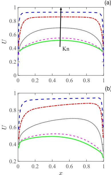
Figure2presents the horizontal velocity on the oscillating lid whent =0 for Ma=0.01 and Ma=1.2, with the Knudsen number from 10 to 0.001. When Ma=0.01, the flow is in the linear oscillation region, and the flow velocity is symmetric along the central vertical line x=0.5L; see Fig. 2(a). As the Knudsen number decreases, the maximum horizontal velocity on the lid increases towards the limitU =U0; this is comprehensible because the smaller the Knudsen number, the smaller the slip velocity is. Also, as Kn decreases, the velocity profile becomes more and more flattened across the center of the lid; this is probably due to the fact that, when Kn is large, the Knudsen layer reaches to the center of the cavity, such that the velocity profile changes rapidly. When Ma=1.2, the flow is in the nonlinear oscillation regime, and the velocity profiles are not symmetrical any more; see Fig.2(b). Instead, when Kn is small (Kn=0.001, 0.01, and 0.1), the maximum flow velocity occurs near the top-right corner of the 2D cavity, while when Kn is large (Kn=1 and 10), the maximum flow velocity occurs close to the cavity center.
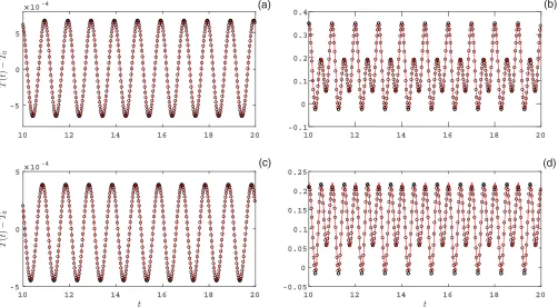
The time evolution of the temperature near the right-top corner of the cavity, e.g., at (x,y)=(0.95L,0.95H), is plotted in Fig.3when Kn=0.1 and 0.01, Ma=0.01 and 1.2, and St= 2. The results with other aspect ratios and Strouhal numbers are similar. When Ma=0.01, it is seen from Figs.3(a)and3(c) that the average temperature variation is zero, while when Ma=1.2, it is seen from Figs.3(b)and3(d)that, most of the time, the top-right corner is heated, which may lead to the burn-ing of this corner. Also, the amplitude of temperature variation for Ma=1.2 is about four orders of magnitude larger than that for Ma=0.01; that is, the variation is roughly proportional to Ma2. With the assistance of the Fourier transform analysis, we note that the temperature evolves with a single frequency the same as the oscillation frequency of the lid when Ma=0.01, but the second-harmonic frequency emerges when Ma=1.2,
0 0.2 0.4 0.6 0.8 1
0 0.2 0.4 0.6 0.8
1 (a)
Kn
0 0.2 0.4 0.6 0.8 1
0.2 0.4 0.6 0.8
1 (b)
FIG. 2. The horizontal velocity on the oscillating lid when
ωt /2π =0, St=2,A=1, and (a) Ma=0.01 and (b) Ma=1.2.
Along the direction of the arrow, the Knudsen number is respectively 10, 1, 0.1, 0.01, and 0.001 for each line. The velocity has been
normalized by the velocity amplitudeU0of the oscillating lid.
which is a strong signature of the nonlinear interaction. The temperature variation is well-fit by a sinusoidal function as
T(t)=a0+a1sin (ωt+φ1)+a2sin (2ωt+φ2), (29)
where the coefficients are given in TableII. Third harmonic or even higher harmonic oscillations are possible when the Mach number increases further.
The influence of the amplitude and frequency of the oscillating lid on the heat transfer is also investigated. Figure4shows the temperature contours overlaid by heat flux streamlines during the first half period when Ma=0.01 and 1.2, Kn=0.1, St=2, andA=1. The temperature variation
T −Tw and flow velocities in the next half period has the same magnitude as in the first half period, but with reversed signs. As shown in Fig. 4(a), when Ma=0.01 and t =0, the moving lid has the maximum velocity, and the cold and hot flow fields appear near the top-left and -right corners of the cavity, respectively. The temperature variation satisfies the symmetry relation T(x,y)−Tw=Tw−T(L−x,y), so that the temperature along the center vertical line x =0.5L
[image:5.608.49.294.120.180.2]10 12 14 16 18 20 -5
0 5
10-4 (a)
10 12 14 16 18 20
-0.1 0 0.1 0.2 0.3
0.4 (b)
10 12 14 16 18 20
-5 0 5 10
-4 (c)
10 12 14 16 18 20
-0.05 0 0.05 0.1 0.15 0.2
[image:6.608.53.555.75.351.2]0.25 (d)
FIG. 3. The evolution of the temperature at (x,y)=(0.95L,0.95H) for (a) Kn=0.1, Ma=0.01, (b) Kn=0.1, Ma=1.2, (c) Kn=0.01,
Ma=0.01, and (d) Kn=0.01, Ma=1.2, with St=2 andA=1. The solid lines are obtained by fitting the numerical results (circle symbol)
with Eq. (29). Note that timethas been normalized by the oscillation period 2π/ω.
temperature and heat flux asymmetrically spread inside the cavity, which is contrary to the case of Ma=0.01 where their distributions are symmetric about the linex =0.5L. In this nonlinear oscillation case, whent =0, the temperature near the top-right corner of the cavity rise rapidly, while that in the top-left corner only decreases slightly; see Fig.4(e). As time goes on, the hot region gradually expands toward the left vertical wall and eventually swap positions with the cold region; see Fig.4(h).
The velocity and frequency of the oscillating lid change the behavior of heat transfer. It is recognized that, for the low-speed rarefied lid-driven cavity flow, the heat could be transferred from the cold to hot region [41,46]; see Fig.5(a), where the Strouhal number is zero. When the lid oscillates, we find from Fig. 4(a) that the direction of heat flux for Ma=0.01 is predominantly from the hot to the cold region at the beginning of a oscillation period, except in the two top corners. When the driving velocity deceases to zero, a heat-transfer circuit emerges near the upper part of the cavity; see Fig.4(c). When Ma=1.2, the hot-to-cold heat transfer
occurs in almost the entire cavity. To assess the influence of the oscillation frequency on the heat-transfer property, we present the temperature contours and the heat flux streamlines att =0, Ma=0.01 and 1.2, and St=0, 0.5, and 1 in Fig.5. As shown, when Ma=0.01, the direction of heat flux for St=0 is generally from the cold to hot flow regions, as is the case of St=0.5. However, when St=1, two heat-transfer circuits appear respectively in the upper and lower parts of the cavity, suggesting a transition of the dominant mechanism in heat transfer. Finally, as observed from Fig.4(a), the hot-to-cold transfer is already prevailing inside the cavity when St=2; this situation does not change when St increases further.
C. Damping force on oscillating lid
We first try to investigate the behavior of the damping force at the limit ofω→ ∞. In this case, binary collisions are
neg-ligible [13] because the high oscillation frequencyωis much larger than the mean collision frequency. As a consequence,
TABLE II. The fitting coefficients corresponding to Eq. (29) when St=2 andA=1.
(Ma,Kn) a0 (a1,φ1) (a2,φ2) ω
(0.01,0.1) 4.502×10⁻⁶ (6.6633×10−4,2.0156) (0,0) 2π
(0.01,0.01) −2.869×10⁻⁵ (4.1864×10−4,2.5843) (0,0) 2π
(1.2,0.1) 0.1442 (0.0840,1.9005) (0.1264,1.3151) 2π
[image:6.608.54.558.676.751.2]X
Y
0.2 0.4 0.6 0.8
0.2 0.4 0.6 0.8
(a) t=0
X
Y
0.2 0.4 0.6 0.8 0.2
0.4 0.6 0.8
t=0.25π (b)
X
Y
0.2 0.4 0.6 0.8 0.2
0.4 0.6 0.8
t=0.5π (c)
X
Y
0.2 0.4 0.6 0.8 0.2
0.4 0.6 0.8
t=0.75π (d)
X
Y
0.2 0.4 0.6 0.8 0.2
0.4 0.6 0.8
t=0 (e)
X
Y
0.2 0.4 0.6 0.8 0.2
0.4 0.6 0.8
t=0.25π (f)
X
Y
0.2 0.4 0.6 0.8 0.2
0.4 0.6 0.8
π
t=0.5 (g)
X
Y
0.2 0.4 0.6 0.8 0.2
0.4 0.6 0.8
[image:7.608.54.557.72.285.2]t=0.75π (h)
FIG. 4. Temperature contours and streamlines of heat flux inside the cavity at different times, when Kn=0.1, St=2,A=1, and the Mach
numbers are Ma=0.01 (top row) and 1.2 (bottom row).
Eq. (5) is equivalent to the collisionless Boltzmann equation:
∂f ∂t +ξx
∂f ∂x +ξy
∂f
∂y =0. (30)
Clearly, the absence of the nonlinear collision term means that the flow system is linear; that is, all the flow properties oscillate around their equilibrium values with the same fre-quencyωof the oscillation lid. Thus, the velocity distribution
function can be expressed as
f(x,y,t,ξ)=feq+Re[exp(iωt)f(x,y,ξ)]U0, (31)
where the equation forfis independent of time:
iStf+ξx ∂f
∂x +ξy ∂f
∂y =0. (32)
X
Y
0.2 0.4 0.6 0.8 0.2
0.4 0.6 0.8
(a)
X
Y
0.2 0.4 0.6 0.8 0.2
0.4 0.6 0.8
(b)
X
Y
0.2 0.4 0.6 0.8 0.2
0.4 0.6 0.8
(c)
X
Y
0.2 0.4 0.6 0.8 0.2
0.4 0.6 0.8
(d)
X
Y
0.2 0.4 0.6 0.8 0.2
0.4 0.6 0.8
(e)
X
Y
0.2 0.4 0.6 0.8 0.2
0.4 0.6 0.8
(f)
FIG. 5. Temperature contours overlaid by the heat flux streamlines inside the cavity for St=0, 0.5 and 1 (from let to right column), and
Ma=0.01 (top row) and 1.2 (bottom row), with Kn=0.1 andA=1, when the horizontal velocity of the lid is maximum along the positive
[image:7.608.56.555.411.713.2]Integrating Eq. (32) with respect to thex, one can obtain
iSt ¯f+ξy ∂f¯
∂y =ξx
f(x=0)−f(x =A)
A , (33)
where ¯f=0Afdx/Ais the average distribution function. Note that Eq. (33) is exactly the same as Eq. (3.3) given by Wu et al. [17] but derived without the assumption of small Mach number. Therefore, for the linear case at high frequency, the right-hand-side of Eq. (33) can be neglected. Hence, together with the boundary condition (24) the analytical solution of the amplitude of the average shear stress on the os-cillating lid can be obtained, which is equal to 1/√π ≈0.564. However, for the nonlinear case, the right-hand-side of Eq. (33) cannot be neglected due to the asymmetrical distributions on the two vertical walls, which results in the asymmetrical distributions of the velocity distribution function; see Fig.2(b) for the velocity profile. Unfortunately it is difficult to derive the analytical solution in this situation, but the numerical results below show that the asymptotic value of the damping force when St→ ∞is very close to that of the linear case.
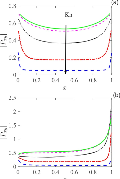
We now numerically solve the Shakhov model at different Knudsen numbers, when St=2, and Ma=0.01 and 1.2, respectively. Results of the shear stress along the oscillating lid are plotted in Fig. 6. It is observed that the shear stress on the lid decreases with the Knudsen number for both linear and nonlinear oscillations, because the corresponding larger velocity at lower Kn should exert a smaller shear stress on the lid. For the linear oscillation, distributions of the shear stress are symmetrical along the linex =0.5L, the same as that of the flow velocity in Fig.2(a). However, for the nonlinear oscillation, distributions of the shear stress are not symmetrical along the center vertical line anymore, and the shear stress adjacent to the right wall is larger than that close to the left wall. For example, when Kn=10, the shear stress near the right wall is about four times that near the left wall.
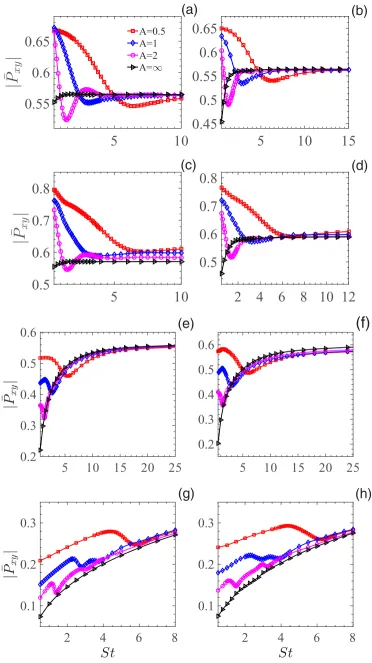
We continue to investigate the variation of the damping force on the oscillating lid as a function of Strouhal number. The results for the linear and nonlinear oscillations at various Knudsen numbers and cavity aspect ratios are plotted in Fig.7. Note that the case of A= ∞corresponds to the 1D oscillatory Couette flow, where the damping force always increases monotonically with Strouhal number. However, the damping force changes nonmonotonically in the 2D cavity. For example, when Kn=0.1 and Ma=0.01, as the Strouhal number increases, the damping force first increases to a local maximum, then decreases to a local minimum, and finally increases toward the limiting value of 1/√π; see Fig. 7(e). Similar behavior is observed in the nonlinear oscillation case, except that the limiting value of the damping force when St→ ∞for Kn=10 and 1 is slightly larger than the analytical value 1/√π, while for Kn=0.1 and 0.01, the limiting value of the damping force is smaller than the analytical solution. Generally speaking, the maximum deviation of the limiting value of the damping force when St→ ∞between Ma=1.2 and 0.01 is less than 7%.
Intuitively, due to the presence of the two vertical walls, the damping force in the 2D oscillatory cavity flow should be larger than that of the 1D oscillating Couette flow. This is indeed the case when the oscillation frequency is small. However,
0
0.2
0.4
0.6
0.8
1
0
0.2
0.4
0.6
0.8
(a)
Kn
0
0.2
0.4
0.6
0.8
1
0
0.5
1
1.5
2
[image:8.608.312.555.76.438.2]2.5
(b)
FIG. 6. The magnitude of shear stress on the oscillating lid when
t=0, St=2, and (a) Ma=0.01 and (b) Ma=1.2. Along the
direction of the arrow, Kn is respectively 10, 1, 0.1, 0.01, and 0.001 for each line. Note that the shear stress has been normalized by
ρ0RTwU0/vm.
as St increases, the damping force in the 2D case could be even smaller than that of the 1D oscillatory Couette flow. For instance, see Fig.7(a), when Kn=10, Ma=0.01 andA=2, the damping force in the oscillatory cavity flow is larger than that of the 1D oscillatory Couette flow when St is less than 1, but above this value, the damping force first decreases to a minimum at St=1.4, and then increases toward the same limits for both the 1D and 2D cases. The underlying physics leading to the minimum in shear stress will be discussed further in the Sec.IV Dbelow.
When Kn=0.01, the variation of amplitude of the average shear stress with respect to the Strouhal number is more complicated than those at larger Knudsen numbers. This situation has not been studied in Ref. [17] because the adopted iterative numerical method can hardly obtain the steady-state solution due to the strong binary collision. However, the explicit DUGKS can handle this problem easily. It is found from Figs. 7(g) and7(h) that, when the cavity aspect ratio
5
10
15
20
25
0.2
0.3
0.4
0.5
0.6
(e)
2
4
6
8
0.1
0.2
0.3
(g)
5
10
15
20
25
0.2
0.3
0.4
0.5
0.6
(f)
2
4
6
8
0.1
0.2
0.3
(h)
5
10
0.55
0.6
0.65
|
¯
P
|
xy
(a)
A=0.5 A=1 A=2
A=∞
5
10
15
0.45
0.5
0.55
0.6
0.65
(b)
5
10
0.5
0.6
0.7
0.8
|
¯
P
|
xy
(c)
2
4
6
8 10 12
0.5
0.6
0.7
[image:9.608.117.489.71.734.2]0.8
(d)
FIG. 7. Variation of the average amplitudes of shear stress on the oscillating lid with St, forA=0.5, 1 and 2, and Kn=10, 1, 0.1, and 0.01
0 0.2 0.4 0.6 0.8 1 1.2 1.4 1.6 0.45
0.5 0.55 0.6 0.65
[image:10.608.51.295.69.285.2]Kn=0.1, St=2 Kn=1, St=2 Kn=0.1, St=10 Kn=1, St=10 Fitting line
FIG. 8. The variation of the amplitude of the average shear stress
on the oscillating lid with the Mach number, when Kn=0.1, 1
and St=2, 10. Note that the shear stress has been normalized by
ρ0RTwU0/vm.
However, whenAis large, the variation of the damping force with respect to the Strouhal number complicates: there are even two local peaks and valleys in the damping force whenA=2. Similar phenomena are observed for Kn=0.001 (not shown here).
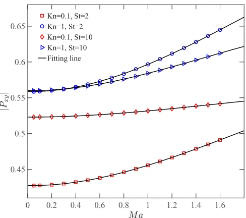
Finally, the variation of the damping force|P¯xy| on the oscillating lid as a function of the Mach number is shown in Fig.8. As expected, the normalized damping force increases monotonically with the Mach number, which is fitted by a three-order polynomial function, with the coefficients listed in TableIII. As the Mach number changes from 0.01 to 1.8, for Kn=0.1 and 1 at St=2, the damping force is increased by more than 20%. However, the variation of the damping force for St=10 is weaker than that of St=2. This is comprehensible because, at large Knudsen numbers, the collision term in the Shakhov model is negligible so that a linear behavior is expected; see Eq. (30).
D. Scaling law for resonance frequency and aspect ratio
The drop (rise) in the amplitude of the average shear stress in Fig.7can be interpreted qualitatively by the gas antiresonance (resonance) inside the cavity [17]. For the free molecular flow, the molecules leaving the top lid with the velocitiesvnearly parallel to the top lid, hitting the right vertical wall, then
TABLE III. Fitting the average shear stress on the oscillating lid
bya3Ma3+a2Ma2+a1Ma+a0.
(Kn,St) a0 a1 a2 a3
(0.1,2) 0.4314 −3.415×10⁻³ 4.174×10⁻² −5.176×10⁻³
(0.1,10) 0.5307 −3.673×10⁻⁴ 1.225×10⁻² −2×10⁻³
(1,2) 0.5649 −1.843×10⁻³ 5.318×10⁻² −7.715×10⁻³
(1,10) 0.5623 −1.819×10⁻³ 3.404×10⁻² −6.89×10⁻³
being reflected and hitting the left vertical wall, and finally returning to the point from which they left, should have traveled a distance about 2L. Thus,
2L≈vδt, (34)
whereδt is the traveling time. Therefore, if
δt =2nπ ω , or
(2n−1)π
ω , n∈Z
+, (35)
then molecules leaving and hitting the top lid should have the same (opposite) phases.
When the velocity distribution functions for molecules leaving and coming back to the oscillating lid are in-phase, the horizontal velocity of the gas near the oscillating lid will be maximum, however, the shear stress defined in Eq. (27) will be minimum, because the molecules leaving and coming back to the lid have opposite y-component velocity. The antiresonance and resonance refer to the states where the shear stress exerting on the oscillating lid are minimum and maximum, respectively. Equations (34) and (35), together with Eq. (2), give the resonance and antiresonance Strouhal numbers as
Str ≈
(2n−1)π
2A v
vm
, n∈Z+, (36)
and
Sta≈ nπ
A v vm
, n∈Z+. (37)
For the linear oscillation, perturbation of the temperature inside the cavity could be neglected, so that the molecular velocity v≈vm(=
√
2RTw). Therefore, the dominant reso-nance Strouhal number Str ≈π/2A and the antiresonance Strouhal number Sta ≈π/Acan be obtained by settingn=1 in Eqs. (36) and (37). On the other hand, for the nonlinear case, as shown in Fig.3, the average temperature inside the cavity is larger than the reference value Tw, so the most probable molecular velocityv=√2RT > vm. As a consequence, Sta and Strshould be larger than that of the linear case.
Note that these analyses are for the free molecular flow. As the Knudsen number decreases, binary collisions of molecules become more intense. Therefore, free transport of the gas molecules is more difficult, so the real traveling time is larger than 2L/v, and the obtained Sta may be smaller than the theoretical values in Eqs. (36) and (37).
To conclude, the antiresonance (resonance) Strouhal num-ber should be related to the degree of gas nonlinearity and rarefaction. On the other hand, the ability of transferring energy from the oscillating lid is boosted by frequent collisions at a smaller Knudsen number, such that the flow inside the cavity could have sufficient kinetic energy to oscillate against the lid. Therefore, the resonance is difficult to develop for the highly rarefied flow, and it is only visible for the small Knudsen number, see Figs.7(g)and7(h).
[image:10.608.359.544.330.395.2] [image:10.608.47.296.681.753.2]0 1 2 3 4 5 -2
0 2 4 6 8 10 12 14
16 (a)
Ma=0.01 DUGKS
Sta=2.91/A-0.21 FSM
Ma=1.2 DUGKS Sta=3.02/A-0.06
0 1 2 3 4 5
0 5 10 15
(b)
Ma=0.01 DUGKS
Sta=3.29/A-0.22 FSM
[image:11.608.109.493.72.256.2]Ma=1.2 DUGKS Sta=3.51/A-0.03
FIG. 9. The antiresonance Strouhal number Sta, at which the amplitude of the average shear stress at the lid is minimum, as a linear function
of the inverse aspect ratio 1/Afor (a) Kn=0.1 and (b) Kn=1. The results of the linearized Boltzmann equation solved by the FSM [17] are
also included for comparison.
because they almost overlap those for Kn=1. It is found that, in the linear case, our simulation results are in excellent agreement with the fitting functions obtained from the FSM solutions. In addition, as expected, the predicted antiresonance Strouhal number Stain the linear oscillation is overall smaller than that of the nonlinear case.
In addition, as we can see from Figs.7(g) and7(h) that for Kn=0.01, both resonance and antiresonance appear, even though their strengths are quite weak relative to the background value. For the first time, we reveal that the linear scaling law for the resonance (antiresonance) Strouhal number and the inverse cavity aspect ratio at Ma=0.01 and 1.2 with Kn=0.01 in
0.5 1 1.5 2 2.5 3 3.5 4 4.5
0 2 4 6 8 10 12 14
Ma=0.01 DUGKS Ma=1.2 DUGKS St
r=1.82/A+0.42 Str=1.79/A+0.45
Sta=2.77/A+0.03
[image:11.608.50.292.468.690.2]Sta=2.94/A+0.03
FIG. 10. The resonance (antiresonance) Strouhal numbers, at which the amplitude of the average shear stress at the lid is a local maximum (minimum), as a linear function of the inverse aspect ratio
1/Awhen Kn=0.01, in both the linear (Ma=0.01) and nonlinear
(Ma=1.2) oscillations.
Fig.10, which is in reasonable agreement with the theoretical Str (Sta) in Eqs. (36) and (37). Furthermore, the fitting lines of the resonant Strouhal number for both linear and nonlinear cases almost overlap each other, suggesting that the velocity amplitude of the lid has little effect on the resonance frequency in the early slip regime.
V. SUMMARY
We have investigated the oscillatory rarefied gas flow in a 2D rectangular cavity on the basis of the Shakhov equation. Both the linear and nonlinear oscillations were numerically studied by using the discrete unified gas-kinetic scheme. The effects of the gas rarefaction, oscillation frequency, and aspect ratio of the cavity were investigated. It has been found that the flow properties, including the flow velocity, temperature, shear stress, and heat flux, are asymmetrically distributed inside the cavity for the nonlinear oscillation, which are different from the linear case where these properties are symmetrical along the vertical centerline of the cavity. Interestingly, it was noticed that the hot-to-cold heat transfer could be dominant inside the linear oscillatory rarefied cavity, which is in contrast to the well-known anti-Fourier (cold-to-hot) heat transfer in a low-speed lid-driven rarefied cavity. For the nonlinear oscillatory flow, the hot-to-cold heat transfer occurs in almost the entire cavity, which is independent of the oscillation frequency. It is also noted that double-frequency oscillation of the temperature evolution is possible in nonlinear oscillation, where the temperature of the top-right corner is significantly higher than the wall temperature in almost the whole oscillation period.
One of the features of the oscillatory cavity flow is that the damping force exerted on the oscillating lid has local dips and peaks when the oscillation frequency changes. This is due to the antiresonance and resonance of rarefied gas flows, respectively. Linear scaling laws for the antiresonance frequency and the inverse aspect ratio of the cavity are established theoretically for the both linear and nonlinear oscillatory flows from the near hydrodynamic to highly rarefied regimes, which are then verified numerically. In particular, the linear scaling law for resonance frequency is also presented in the early slip regime, where the resonance is easy to develop.
The present study provides a useful guideline to avoid damping damage induced by the nonlinear oscillation for design of MEMS devices.
ACKNOWLEDGMENT
This work is financially supported by the UK’s Engineering and Physical Sciences Research Council (EPSRC) under grants EP/M021475/1, EP/L00030X/1.
[1] G. Karniadakis, A. Beskok, and N. Aluru, Microflows and
Nanoflows: Fundamentals and Simulation(Springer, New York, 2005).
[2] S. Chigullapalli, A. Weaver, and A. Alexeenko,J. Micromech.
Microeng.22,065010(2012).
[3] J. H. Park, P. Bahukudumbi, and A. Beskok,Phys. Fluids16,
317(2004).
[4] A. Frangi, A. Frezzotti, and S. Lorenzani,Comput. Struct.85,
810(2007).
[5] D. Kalempa and F. Sharipov,Phys. Fluids21,103601(2009).
[6] F. Sharipov, Rarefied Gas Dynamics: Fundamentals for
Re-search and Practice(John Wiley & Sons, 2015).
[7] S. Stefanov, P. Gospodinov, and C. Cercignani,Phys. Fluids10,
289(1998).
[8] N. G. Hadjiconstantinou,Phys. Fluids14,802(2002).
[9] J. H. Park, S. W. Baek, S. J. Kang, and M. J. Yu,Numer. Heat
Transfer, Part A42,647(2002).
[10] J. H. Park and S. W. Baek,Int. J. Heat Mass Transfer47,1313
(2004).
[11] N. G. Hadjiconstantinou and A. L. Garcia,Phys. Fluids13,1040
(2001).
[12] D. R. Emerson, X.-J. Gu, S. K. Stefanov, S. Yuhong, and R. W.
Barber,Phys. Fluids19,107105(2007).
[13] F. Sharipov and D. Kalempa, Microfluid. Nanofluid. 4, 363
(2008).
[14] D. Kalempa and F. Sharipov,Int. J. Heat Fluid Flow38,190
(2012).
[15] T. Doi,Vacuum84,734(2009).
[16] T. Tsuji and K. Aoki,Microfluid. Nanofluid.16,1033(2014).
[17] L. Wu, J. M. Reese, and Y. Zhang,J. Fluid Mech.748, 350
(2014).
[18] F. Sharipov, W. Marques Jr., and G. Kremer,J. Acoust. Soc. Am.
112,395(2002).
[19] L. Wu,Phys. Rev. E94,053110(2016).
[20] F. Sharipov and D. Kalempa,J. Acoust. Soc. Am.124,1993
(2008).
[21] Y. W. Yap and J. E. Sader,Phys. Fluids24,032004(2012).
[22] N. G. Hadjiconstantinou,Phys. Fluids17,100611(2005).
[23] L. Wu, C. White, T. J. Scanlon, J. M. Reese, and Y. Zhang,
J. Comput. Phys.250,27(2013).
[24] L. Wu, J. M. Reese, and Y. Zhang,J. Fluid Mech.746,53(2014).
[25] J. Iannacci, M. Huhn, C. Tschoban, and H. Pötter,IEEE Electron
Device Lett.37,1646(2016).
[26] J. Nassios and J. E. Sader,J. Fluid Mech.729,1(2013).
[27] K. Aoki, S. Kosuge, T. Fujiwara, and T. Goudon, Phys. Rev.
Fluids2,013402(2017).
[28] S. Wang, L. Baldas, S. Colin, S. Orieux, A. Kourta, and N.
Mazellier, in8th AIAA Flow Control Conference (American
Institute of Aeronautics and Astronautics, Washington, D.C., 2016). p. 4234.
[29] C.-M. Ho and Y.-C. Tai,Annu. Rev. Fluid Mech.30,579(1998).
[30] J. Miau, T. Leu, J. Yu, J. Tu, C. Wang, V. Lebiga, D. Mironov,
A. Pak, V. Zinovyev, and K. Chung,Sens. Actuators, A235,1
(2015).
[31] E. Shakhov,Fluid Dyn.3,95(1968).
[32] J. Yang and J. Huang,J. Comput. Phys.120,323(1995).
[33] Z. Guo, K. Xu, and R. Wang,Phys. Rev. E88,033305(2013).
[34] Z. Guo, R. Wang, and K. Xu, Phys. Rev. E 91, 033313
(2015).
[35] P. Wang, L. Zhu, Z. Guo, and K. Xu,Commun. Comput. Phys.
17,657(2015).
[36] P. Wang, S. Tao, and Z. Guo,Comput. Fluids120,70(2015).
[37] L. Zhu, P. Wang, and Z. Guo,J. Comput. Phys.333,227(2017).
[38] Y. Bo, P. Wang, Z. Guo, and L.-P. Wang,Comput. Fluids155,9
(2017).
[39] P. Wang, L.-P. Wang, and Z. Guo,Phys. Rev. E 94,043304
(2016).
[40] P. Wang, M. T. Ho, L. Wu, Z. Guo, and Y. Zhang,Comput. Fluids
161,33(2017).
[41] L. Zhu, Z. Guo, and K. Xu,Comput. Fluids127,211(2016).
[42] L. Zhu and Z. Guo, Comput. Fluids (2017), doi:
10.1016/j.compfluid.2017.09.019.
[43] Z. Guo and K. Xu, Int. J. Heat Mass Transfer 102, 944
(2016).
[44] P. Wang, Y. Zhang, and Z. Guo,Int. J. Heat Mass Transfer113,
217(2017).
[45] W. Su, S. Lindsay, H. Liu, and L. Wu,Phys. Rev. E96,023309
(2017).
[46] B. John, X.-J. Gu, and D. R. Emerson,Numer. Heat Transfer,