City, University of London Institutional Repository
Citation
:
Pattni, K., Broom, M. & Rychtar, J. (2017). Evolutionary dynamics and the
evolution of multiplayer cooperation in a subdivided population. Journal of Theoretical
Biology, 429, pp. 105-115. doi: 10.1016/j.jtbi.2017.06.034
This is the accepted version of the paper.
This version of the publication may differ from the final published
version.
Permanent repository link: http://openaccess.city.ac.uk/17811/
Link to published version
:
http://dx.doi.org/10.1016/j.jtbi.2017.06.034
Copyright and reuse:
City Research Online aims to make research
outputs of City, University of London available to a wider audience.
Copyright and Moral Rights remain with the author(s) and/or copyright
holders. URLs from City Research Online may be freely distributed and
linked to.
Evolutionary dynamics and the evolution of multiplayer
cooperation in a subdivided population
Karan Pattnia, Mark Brooma, Jan Rycht´aˇrb
aDepartment of Mathematics, City, University of London, Northampton Square, London,
EC1V 0HB, UK
bDepartment of Mathematics and Statistics, The University of North Carolina at
Greensboro, Greensboro, NC 27412, USA
Abstract
The classical models of evolution have been developed to incorporate structured populations using evolutionary graph theory and, more recently, a new frame-work has been developed to allow for more flexible population structures which potentially change through time and can accommodate multiplayer games with variable group sizes. In this paper we extend this work in three key ways. Firstly by developing a complete set of evolutionary dynamics (BDB, BDD, DBD, DBB, LB and LD) so that the range of dynamic processes used in classical evolution-ary graph theory can be applied. Secondly, by building upon previous models to allow for a general subpopulation structure, where all subpopulation members have a common movement distribution. Subpopulations can have varying lev-els of stability, represented by the proportion of interactions occurring between subpopulation members; in our representation of the population all subpopula-tion members are represented by a single vertex. In conjuncsubpopula-tion with this we extend the important concept of temperature (the temperature of a vertex is the sum of all the weights coming into that vertex; generally, the higher the temperature, the higher the rate of turnover of individuals at a vertex). Finally, we have used these new developments to consider the evolution of cooperation in a class of populations which possess this subpopulation structure using a multiplayer public goods game. We show that cooperation can evolve providing that subpopulations are sufficiently stable, with the smaller the subpopulations the easier it is for cooperation to evolve. We introduce a new concept of tem-perature, namely “subgroup temperature”, which can be used to explain our results.
1. Introduction 1
Evolutionary game theory has proved to be a very successful way of
mod-2
elling the evolution of, and behaviour within, populations. The classical models
3
mainly focused on well-mixed populations playing two player games [31, 30], or
4
alternatively playing games against the entire population [30]. Simple models
5
such as the Hawk-Dove game [29] and the sex ratio game [20] have been used
6
to explain important biological phenomena.
7
These models were developed to consider finite populations explicitly [34,
8
Chapters 6-9] (although see [32, 33] for important earlier non-game theoretic
9
work) and structured populations using the now widespread methodology of
10
evolutionary graph theory originated in [26] (see also [3, 9, 52, 27], and [1, 44]
11
for reviews). Such population structures can have a profound effect on the result
12
of the evolutionary process even when individuals have a fixed fitness [26, 28, 40].
13
Further, even for a given structure, the rules of the evolutionary dynamics have
14
a significant effect on the evolution of the population.
15
Previous work has investigated a number of important questions, the most
16
widely considered being how cooperation can evolve. The evolution of
cooper-17
ation, where individuals make sacrifices to help others, can seem paradoxical
18
within the context of natural selection, especially amongst unrelated
individu-19
als. There are a number of ways that mathematical modelling has demonstrated
20
that cooperation can occur [35]; one key way is through the presence of
popula-21
tion structure, which can mean that cooperative individuals are more likely to
22
interact with other cooperators, which makes them resistant to exploitation by
23
defectors [36, 42]. In particular, this is true for structures where individuals are
24
heterogeneous [43] allowing hubs or clusters of cooperators to form. The
dynam-25
ics that one uses are also important; for example [36] showed that death-birth or
26
birth-death dynamics with selection on the second event promotes cooperation
27
but not when selection happens in the first event.
28
One limitation of evolutionary graph theory is that it naturally lends itself
29
to pairwise games, whereas real populations can often involve the simultaneous
30
interaction of many individuals [45, 15]. Multiplayer games, whilst more
com-31
mon in economic modelling [21, 6], have become used in increasing frequency
32
within evolutionary games starting with [38, 7] (see also [14, 18]) and it is
im-33
portant to incorporate these too into the modelling of structured populations.
34
A multiplayer public goods game [4, 5, 19, 54], (and this type of game is central
35
to our paper too, see Section 2.4) has been used in evolutionary graph theory
36
[25, 51, 24, 41, 56], but this typically involves forming an individual and all of
37
its neighbours into a group and allowing them to play a game. Although this is
38
convenient, it is not really natural because there is no mechanism for deciding
39
how individuals spend their time, and so how they share that time with others,
40
either singly or in groups.
41
More recently a general framework has been developed [10, 13, 8, 11] which
42
considers the interaction of populations in a more flexible way, where groups of
43
any size can form, with different propensity potentially depending upon a
num-44
ber of factors, including the history of the process. Crucially, the key elements
45
of evolutionary graph theory of population structure, game and evolutionary
46
dynamics occur for this new framework too; this makes it capable of analysing
47
different spatial structures whilst providing the flexibility for different
multi-48
player interactions. Prior to the current paper, the actual applications of the
P1 P2 Pm−1 Pm Pm+1 PM−1 PM
I1 I2 In IN
p1,1
p2,1
p2,2
p1,m−1
pn,m
pn,m+1
pN,M−1
[image:4.612.173.441.123.241.2]pN,M
Figure 1: The fully independent model from [10]. There areNindividuals who are distributed overM places such thatInvisits placePmwith probabilitypnm. Individuals interact with one another when they meet, for example,I1andI2can interact with one another when they meet inP1.
above framework have been limited. In particular only a single evolutionary
50
dynamics (the BDB dynamics from the current paper) has been used, and only
51
relatively simple populations, which resembled those in evolutionary graph
the-52
ory (the population consisting of individuals each resident at a unique graph
53
vertex) have been considered.
54
In this paper we further develop the general theory of the framework
orig-55
inated in [10]. We first show how to represent subpopulations using a reduced
56
graphical representation within our structure, which will then allow us to
po-57
tentially consider larger populations with a richer structure than previously. We
58
then demonstrate how to apply a standard set of evolutionary dynamics to
con-59
sider a range of evolutionary processes. This is vital since, as mentioned above,
60
dynamics can have a big effect on the outcome of evolution within other models,
61
including evolutionary graph theory, and as we will see, this is certainly also
62
true for our work. Finally we use these new tools to consider the evolution of
63
cooperation using a multiplayer public goods game [51, 48, 49, 4] and show that
64
cooperation can occur when both the structure and evolutionary dynamics act
65
together in favour of the cooperators.
66
The paper is structured as follows: in Section 2 the model framework is
67
described, including how to incorporate subpopulations. In Section 3 a standard
68
set of evolutionary dynamics to be used with our model are defined. In Section
69
4 we introduce and discuss the important concepts of fixation probability and
70
temperature. In Section 5 we study the evolution of cooperation in our model
71
with subpopulations. Section 6 is then a general discussion.
72
2. A framework for modelling evolution in structured populations 73
A framework for modelling the movement of individuals was presented in
74
[10]. This is a very general and flexible methodology, the details of which are
75
not necessary for the current paper. Below we describe the fully independent
76
version of this framework in which individuals move independently of each other
Table of Notation
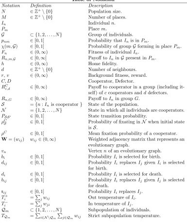
Notation Definition Description
N ∈Z+\ {0} Population size.
M ∈Z+\ {0} Number of places.
In Individualn.
Pm Placem.
G ⊂ {1,2, . . . , N} Group of individuals.
pnm ∈[0,1] Probability thatIn is in Pm.
χ(m,G) ∈[0,1] Probability of groupGforming in placePm. Fn ∈(0,∞) Fitness of individualIn.
Rn,m,G ∈[0,∞] Payoff toIn in G present inPm. h ∈(0,∞) Home fidelity.
d ∈Z+\ {0} Number of neighbours.
r,v ∈(0,∞) Background fitness, reward.
C, D Cooperator, Defector.
RC
c,d ∈[0,∞) Payoff to cooperator in a group (including
it-self) ofc cooperators andddefectors.
Rn,G ∈[0,∞) Payoff toIn in groupG.
S ={n:In is cooperator} State of the population.
N ={1,2, . . . , N} State in which all individuals are cooperators.
PSS0 ∈[0,1] State transition probability.
ρC
S ∈[0,1] Probability of fixating inN when initial state isS.
ρC ∈[0,1] Mean fixation probability of a cooperator. W= (wij) wij ∈(0,∞) Weighted adjacency matrix that represents an
evolutionary graph.
vn Vertexnof an evolutionary graph. bi ∈[0,1] ProbabilityIi is selected for birth.
dij ∈[0,1] Probability Ii replacesIj given Ii is selected
for birth.
di ∈[0,1] ProbabilityIi is selected for death.
bij ∈[0,1] Probability Ii replaces Ij given Ij is selected
for death.
rij ∈[0,1] ProbabilityIi replacesIj.
Ti+ =P
jwij Out temperature ofIi.
Ti− =
P
jwji In temperature ofIj.
Qm ⊂ {1,2, . . . , N} Subpopulation of individuals.
TQm =
P
i∈N \Qm
P
j∈Qmwij Strict subpopulation temperature. Table 1: Notation used in the paper.
and independently of the population’s history (any past movements). Important
78
terms used in the current paper are given in Table 1.
2.1. The fully independent model 80
The population is made up ofNindividualsI1, . . . , IN who can move around 81
M places P1, . . . , PM. The probability of individual In being at place Pm is 82
denoted by pnm; see Figure 1 for a visual representation using a bi-partite 83
graph. When individuals move around they form groups. Let G denote any
84
group of individuals, then the probabilityχ(m,G) that groupG forms in place
85
Pm is given by 86
χ(m,G) =Y
i∈G
pim
Y
j /∈G
(1−pjm). (2.1) 87
88
We can show from equation (2.1) that
89
1 =X
m
X
G
n∈G
χ(m,G) ∀n. (2.2)
90
91
This follows intuitively from the fact that individualInhas to be present in some 92
placePmin some groupG at any given time. The mean size of an individual’s 93
group (see also [13]) is given by
94
¯
G=X
m
X
G
χ(m,G)|G|2
P
m
P
Gχ(m,G)|G| =X
m
X
G
χ(m,G)|G|2
N (2.3)
95
96
where the simplification of the denominator follows from equation (2.2).
97
When a group of individuals is formed they will then interact with one
98
another. In particular, individual In will receive a payoff that depends upon 99
the group G it is present in and the place Pm occupied by this group. This 100
is denoted as Rn,m,G and was referred to in [10] as a direct group interaction
101
payoffbecause individualIn only interacts with other individuals with whom it 102
is directly present with ([10] allowed for a more general class of payoff but this
103
is the only type we will consider, and hence will just refer to it as the payoff).
104
IndividualIn’s fitness is then calculated by averaging its payoffs over all possible 105
groups and places that these groups can form as follows:
106
Fn =
X
m
X
G
n∈G
χ(m,G)Rn,m,G. (2.4)
107
A version of the fully independent model called the territorial raider model
108
was introduced in [10] and further developed in [8]. A generalization of this
109
model forms the basis of much of the work in this paper, although we note that
110
Section 3 in particular is more general.
111
2.2. The territorial raider model 112
In the territorial raider model, each individualIn has its own placePn with 113
no unoccupied places and, therefore, there is a one-to-one correspondence
be-114
tween individuals and places. A graph is used to represent the structure of the
Figure 2: The territorial raider model of [10, 8]. (a) Population structure represented using a graph where vertices represent individuals and places. IndividualInlives in placePnand can visit any neighbouring places. For example, the home place ofI1is placeP1 but it can visit placesP2, P3andP4. (b) An alternative visualization on a bi-partite graph where individuals and places are clearly separated.
population where each vertex represents an individual and its corresponding
116
home such that two connected individuals can raid each others home places
117
(see Figure 2). The probability of raiding another’s home place is governed by
118
a common movement parameter called home fidelity, h, that measures an
in-119
dividuals’ preference for their home place. In particular, an individual withd
120
neighbours would stay on their home place with probability h/(h+d) or raid
121
any one of its neighbours’ home places with an equal probability of 1/(h+d)
122
(see Figure 2).
123
I1, I2 I3, I4 I5
(a)
I1 I2 I3 I4 I5
P1 P2 P3
(b)
Figure 3: The generalized territorial raider model. (a) Individuals that are members of sub-populationQmlive in placePmbut can visit neighbouring places. The territory of subpop-ulation{I1, I2}consists of placesP1 andP2, the territory of subpopulation{I3, I4}consists of placesP1, P2 and P3, the territory of subpopulation{I5} consists ofP2 andP3. (b) An alternative visualization as multiplayer interactions on a bi-partite graph where individuals and places are clearly separated.
2.3. The generalized territorial raider model 124
In this section we generalise the territorial raider model to include
subpopu-125
lations, based upon their movement distributions. We will see that individuals
126
within a given subpopulation are more likely to interact with each other than
127
with members of other subpopulations, and this will affect the success of their
128
strategies.
[image:7.612.164.446.404.504.2]Consider the fully independent model. We define a subpopulation of
individ-130
uals as a division of individuals from the main population that iswell-mixed[10],
131
which simply means that all of these individuals have an identical distribution
132
over the places. In particular, for a subpopulationQwe have that pim =pjm 133
∀ i, j ∈ Q and m = 1, . . . , M. This can be visualised in terms of a bipartite
134
graph as in Figure 1 where theI-vertices are now occupied by subpopulations
135
rather than individuals. This subpopulation structure is thus a special case of
136
the fully independent model.
137
For simplicity we will assume that individuals move as they do in the
terri-138
torial raider model; thus our model is a generalization of the territorial raider
139
model. A population ofN individuals is divided intoM non-overlapping
sub-140
populations Q1, . . . ,QM where |Qm| ≥ 0 such that N = Pm|Qm|. We will 141
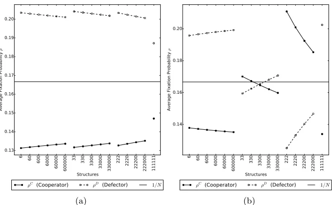
assume that individuals in subpopulation Qm treat place Pm as their home 142
place, so that there is a one-to-one correspondence between subpopulations and
143
places. However, because we allow subpopulations to be empty, we can have
144
places in which no individuals reside. As before, the movement probabilities of
145
the individuals is governed by the home fidelityh. In particular, a
subpopula-146
tionQm that can visitdneighbouring places will stay in home place Pm with 147
probabilityh/(h+d) or move to one of its neighbouring places with probability
148
1/(h+d). Note that when there is one individual in each subpopulation, that
149
is |Qm| = 1 ∀m, we recover the territorial raider model in Section 2.2. This 150
information can be visually represented in two different ways as shown in
Fig-151
ure 3, which includes a graph whose vertices represent both subpopulations and
152
places. This generalized territorial raider model will be the basis of our detailed
153
investigation of the evolution of cooperation in Section 5.
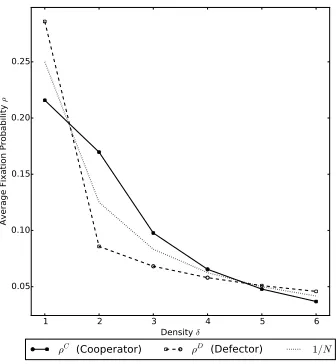
154
2.4. A multiplayer public goods game 155
A multiplayer Hawk-Dove game [46] and a public goods game were
con-156
sidered in [8], though there are other games that can be considered like the
157
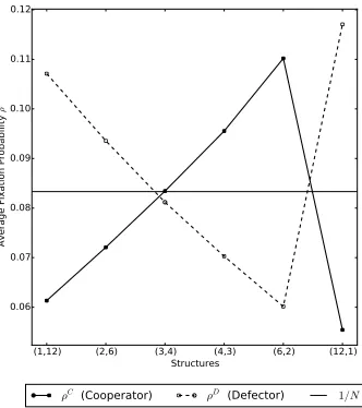
multiplayer stag hunt game [37].
158
In this paper we focus only on the multiplayer public goods game based on
159
the game defined by [51], where an individual’s payoff is an average of two player
160
public goods games (just a version of the standard prisoner’s dilemma) played
161
with each of its group mates. Players can either cooperate (C) or defect (D).
162
A cooperator always pays a cost 1 so that the other player receives a reward
163
v and a defector pays no cost but only receives a reward when present with a
164
cooperator. Note that the cost is set to 1 because scaling all the payoffs by
165
some other cost value does not affect the outcome of the game and, therefore,
166
the rewardv is a multiple of the cost. The payoff matrix is thus given by
167
C D
C v−1 −1
D v 0
. (2.5)
168
169
In [51] and most models involving public goods games, individuals are never
170
alone, and so what happens in the case they are alone is not considered.
How-171
ever, in our case it is possible for an individual to be alone, for example, an
individual could remain on its home place and not be raided. As in [8], we will
173
assume that a lone cooperator still pays a cost but does not receive a reward
174
and lone defectors receive nothing. There are other ways that we can allocate
175
rewards to lone individuals; for example, in [22] there is a specific strategy, the
176
loner strategy, where cooperators choose to be alone and not pay a cost. Our
177
choice seems a natural generalisation of the prisoners dilemma model [51], where
178
individuals pay a cost but do not benefit from their own contributions. We note
179
that our version makes cooperation harder to evolve than the alternatives. Thus
180
if cooperators thrive in a population using our model, this can be thought of as
181
strong support for the evolution of cooperation.
182
In the multiplayer public goods game, the payoffs to cooperators and
defec-183
tors playing within a group ofc cooperators and ddefectors (including
them-184
selves) is then respectively given by
185
RC
c,d=
(
r−1, c= 1
r−1 +c+c−d−11v, c >1 and R
D c,d=
(
r, c= 0
r+c+dc−1v, c >0 (2.6)
186
187
whereris a background payoff, which is also a multiple of the cost, that every
188
individual receives, representing the contribution from activities that are not
189
related to the games. Generally, the effect of selection is weaker the larger
190
the value ofr (for example, see [12], Chapter 2). The payoff is then given by
191
Rn,m,G ≡RCc,d(≡Rc,dD) whenInis a cooperator (defector) and|G|=c+d, which 192
can then be substituted into Equation 2.4 to find the individual’s fitness. Note
193
that here the payoffs do not depend upon the place occupied by the individuals,
194
that is,Rn,m,G≡Rn,G.
195
3. Evolutionary dynamics 196
In this section we revisit the standard dynamics of evolutionary graph theory,
197
before demonstrating how we can adapt each of them to our framework. For
198
the current work there will actually only be two distinct dynamics, but for more
199
general cases each will be distinct, and so it is important to consider them all.
200
We start by recalling the dynamics from evolutionary graph theory.
201
3.1. Evolutionary dynamics in evolutionary graph theory 202
An evolutionary graph [26, 40] is a graph represented by a weighted
adja-203
cency matrix W= (wij) where wij ∈ [0,∞) is referred to as the replacement 204
weight. Each vertexvn of the evolutionary graph is occupied by one individual 205
and if wij > 0 then the individual on vi can place a copy of itself in vj by 206
replacing the individual there. It is assumed that the weights are chosen so that
207
the evolutionary graph is strongly connected, which means that there is a route
208
of finite length between any pair of verticesvi andvj. The weighted adjacency 209
matrixWis therefore said to define the replacement structure.
210
Assuming that there is only one replacement per update event, there are
211
Dynamics
BDB bi= PFi
nFn
, dij = Pwij
nwin
BDD bi= 1
N, dij =
wijFj−1
P
nwinFn−1
DBD dj =
Fj−1
P
nF−
1
n
, bij =
wij
P
nwnj
DBB dj=
1
N, bij =
wijFi
P
nwnjFn
LB rij =
wijFi
P
n,kwnkFn
LD rij =
wijFj−1
P
[image:10.612.138.476.124.230.2]n,kwnkFk−1
Table 2: Dynamics defined using the replacement weight as in [40]. In each case, B (D) is appended to the name of the dynamics if selection happens in the birth (death) event.
where a copy of the individual onvireplaces the individual onvj. In particular, 213
we can broadly classify these in terms of the order in which vi and vj are 214
picked. For birth-death dynamics (BD) the birth event happens first where the
215
individual on vi is chosen for birth with probability bi. The individual on vj 216
is then chosen for death conditional on the individual onvi giving birth with 217
probabilitydij, thusrij =bidij. For death-birth dynamics (DB) the death event 218
happens first where the individual onvj is chosen for death with probability 219
di. The individual on vi is then chosen for birth conditional on the death of 220
individual on vj with probability bij, thus rij =dibij. For link dynamics (L) 221
both birth and death events happen simultaneously and thereforerij cannot be 222
decomposed.
223
For each of these dynamics, natural selection can influence the birth (‘B’
ap-224
pended to name) or death (‘D’ appended to name) event. We use the definitions
225
of [28] who extensively studied a set of each of these dynamics. In terms of the
226
exact formulae of the transition probabilities, we use those of [40] as summarised
227
in Table 2. In these definitions, the dynamics are a function of the replacement
228
structure W and the fitnesses of the individuals such that the individual on
229
vertexvn has fitness Fn. 230
3.2. Evolutionary dynamics in our framework 231
In [8] a birth-death dynamics was defined to be used with the territorial
232
raider model. In this section we shall develop a consistent set of dynamics
233
for our framework. In particular, we will show that we can adapt the above
234
dynamics widely used in evolutionary graph theory.
235
To consider the evolution of the population it is useful to think of the
in-236
dividuals in the population in an abstract way. In particular, individuals in
237
the population change through time and, therefore, it is better to think of Ii 238
as a position that an individual can occupy. These positions are referred to
239
as I-vertices in [8] and have a particular relationship to the places, although
240
as the population evolves the actual individual, and in particular the type of
241
individual, occupying the position may change. We will generally simply refer
242
to theseI-vertices as “individuals” but make the distinction where necessary.
This leads to a natural way to create evolutionary dynamics for our
frame-244
work; namely, by mapping each individual Ii to vertex vi, we can incorporate 245
the replacement weights of different interaction methods straight into the
for-246
mulae from Table 2. All that remains is to choose the replacement weights
247
appropriately.
248
The replacement weights used here are based on the assumption that an
249
offspring of individualIi is likely to replace another individualIj proportional 250
to the timeIi and Ij spend together. The offspring of Ii can also replace Ii 251
itself and it does this proportional to the timeIispends alone. Therefore, when 252
i6=j, the probability thatIi andIj meet is given by summingχ(m,G) over all 253
msuch that i, j∈ G. When they meet, we assume thatIi will spend an equal 254
amount of time with each other individual in groupG and, therefore, weight
255
χ(m,G) with 1/(|G| −1) since there are|G| −1 other individuals (an alternative
256
weighting could be 1/|G|that allows interaction within groups larger than one
257
to contribute to the probability ofIi’s offspring replacing itself). Note that this 258
is consistent with the payoffs from our public goods game, where each pairwise
259
payoff equally contributes to the total payoff an individual receives. On the
260
other hand, when i= j, we sumχ(m,G) over all m such thatG = {i}. Here
261
there is no need to weightχ(m,G) becauseIi is alone. 262
The replacement weights are therefore calculated as follows
263
wij =
X
m
X
G
i,j∈G
χ(m,G)
|G| −1 i6=j,
X
m
χ(m,{i}) i=j.
(3.1)
264
265
Thus we have a new set of evolutionary dynamics which can be applied to
266
our framework in a wdie variety of situations (including those that we consider
267
later in this paper). Note that the dynamics used in [8] is the BDB dynamics
268
defined from the above process.
269
By our definition W is symmetric, that is wij = wji ∀i, j, because the 270
probability ofIi meeting Ij within any given group is clearly the same as that 271
ofIjmeetingIi. We also have thatWis doubly stochastic, that is 1 =Pjwij = 272
P
iwij for alli, j, becausewij is the proportion of timeIi spends withIj (with 273
wii the proportion of time it spends alone), and it is always in precisely one of 274
theseN categories. In this case,Wis referred to as beingisothermal [26, 40].
275
We note that the results above hold because of the particular weightswijthat 276
we have chosen. Although these are natural, they are not the only possibility.
277
In particular we could have alternative weights where wij and wji are not in 278
general equal and/or whereWis not isothermal.
279
4. Fixation probability and the temperature 280
4.1. The fixation probability 281
The (mean)fixation probabilityρC (ρD) is the probability that the offspring 282
of a randomly placed mutant cooperator (defector) eventually replaces the entire
population. This can be uniformly at random as in [26]; alternatively, one can
284
use themutant appearance distributionas described in [2]. [8] used a version of
285
this where they weighted the fixation probabilities using the mean temperature.
286
For this current work we use the arithmetic mean, as the difference between
287
these two approaches is negligible here, with the arithmetic mean being greater
288
than or equal to the weighted mean [2]. For more details on how the fixation
289
probability is calculated, see the Appendix.
290
As in [50], we will use the neutral fixation probability 1/N as a benchmark
291
when comparing cooperators and defectors using their fixation probabilities. In
292
particular, [50] say thatselection opposes D replacing C when ρC <1/N and 293
selection favoursC replacingD when 1/N < ρC. It is said that typeCevolves 294
if both these conditions hold, i.e. if
295
ρD<1/N < ρC. (4.1)
296 297
4.2. Concepts of temperature 298
In [26] thein temperature (or just the temperature) of a vertex of an
evo-299
lutionary graph was introduced to measure how likely an individual occupying
300
a particular vertex is to be replaced by another individual’s offspring. [28]
301
extended this definition and introduced the out temperature of a vertex of an
302
evolutionary graph to measure how likely the offpsring of the individual
occupy-303
ing that vertex will replace another individual. These definitions of the in and
304
out temperatures of individualIn for an evolutionary graphWare respectively 305
defined as follows
306
Tn− =
X
i
win and Tn+=
X
i
wni. (4.2) 307
308
In general, the in and out temperatures can be different. However, in our
309
case, W is doubly stochastic and symmetric and, therefore, the in and out
310
temperatures are identical. We therefore work with the definition of only in
311
temperature and simply refer to it as the temperature.
312
An alternative version of the definition of temperature (used in [8]) is the
313
stricttemperature that measures how often an individual is likely to be replaced
314
by other individuals excluding itself. SinceW is doubly stochastic, the strict
315
temperature of individualIn for an evolutionary graphWis given by 316
Tn=
X
i6=n
win= 1−wnn. (4.3) 317
318
The definition of strict temperature can be extended to subpopulations to
319
give the strict subpopulation temperature. This measures how likely an
in-320
dividual in subpopulation Qm is to be replaced by an individual in another 321
subpopulation. Clearly all individuals in a subpopulation have the same
tem-322
perature (for any of our temperature definitions), since they all have the same
323
movement distribution. The strict subpopulation temperature is calculated by
6 60 600 6000
60000 600000 33 330
3300 33000
330000
222 2220 22200 222000 111111 Structures
0.13 0.14 0.15 0.16 0.17 0.18 0.19 0.20
Av
er
ag
e F
ixa
tio
n
Pr
ob
ab
ilit
y
ρ
ρC (Cooperator) ρD (Defector) 1/N
(a)
6 60 600 6000
60000 600000 33 330
3300 33000
330000
222 2220 22200 222000 111111 Structures
0.14 0.16 0.18 0.20
Av
er
ag
e F
ixa
tio
n
Pr
ob
ab
ilit
y
ρ
ρC (Cooperator) ρD (Defector) 1/N
[image:13.612.137.476.122.332.2](b)
Figure 4: Comparing average fixation probability for different complete structures where fig-ure (a) uses DBD dynamics and figfig-ure (b) uses DBB dynamics. Each number indicates a subpopulation of a certain density. For example 60 is a complete structure with 2 subpopu-lations of size 6 and 0 respectively; 2220 has three subpopusubpopu-lations of size 2 and one of size 0. In each case the public goods game parameters arer= 30, v= 10 and movement parameter ish= 30. We see that in figure (a) for the DBD dynamics, cooperators perform poorly in all cases. In figure (b), cooperators do better for small groups (greater than one). Increasing the number of empty places is beneficial for defectors.
summing all weightswij such thatIi is not part of subpopulationQmandIj is 325
part of subpopulationQmgiving 326
TQm =
X
i∈N \Qm
X
j∈Qm
wij. (4.4)
327
328
This means that if there is only one subpopulation then its strict subpopulation
329
temperature is 0 by definition, that is,TQm = 0 ifQm=N.
330
We note that a strategy introduced in one subpopulation can spread
through-331
out the population becauseWis strongly connected. This implies that if there
332
is more that one non-empty subpopulation then the strict subpopulation
tem-333
perature is non-zero for all non-empty subpopulations, that is, TQm > 0 if
334
|Qm| > 0. To measure the connectedness of the subpopulations, that is how 335
often the different subpopulations interact with one another, we use the mean
336
strict subpopulation temperature that is defined as follows
337
hTQmi=
1
N M
X
m=1
|Qm|TQm. (4.5)
338
1 2 3 4 5 6 Density δ
0.05 0.10 0.15 0.20 0.25
Av
er
ag
e F
ixa
tio
n
Pr
ob
ab
ilit
y
ρ
[image:14.612.136.304.123.305.2]ρC (Cooperator) ρD (Defector) 1/N
Figure 5: Comparing average fixation probability for differentδthat is the size (or density) of each subpopula-tion in a complete graph with 4 sub-populations. The public goods game parameters are set tor= 30, v= 11, the movement parameters are set to
h= 30 and dynamics used are DBB. As in Figure 4, cooperators evolve better in small groups (larger than 1), namely groups of size two and three, with a small advantage for groups of size four.
5. Cooperation in generalized territorial raider models 340
In this section we study the effect that different model parameters have
341
on the evolution of cooperation. For models investigating the evolution of
co-342
operation using evolutionary graph theory, both the evolution and interaction
343
of individuals are dictated by a fixed structure, following games with a fixed
344
number of players (almost always two). In our model the replacement
struc-345
ture emerges from the interactions between individuals, involving games with a
346
varying number of players, and therefore give us a different perspective on the
347
evolution of cooperation.
348
5.1. The effect of the dynamics 349
As we mentioned in Section 1, for evolutionary graph theory models,
coop-350
eration is favoured when using DBB or BDD dynamics, but not DBD or BDB
351
dynamics, if the structure allows a cluster of cooperators to form (also see [36]).
352
This is consistent with [8] where we studied the effect of the BDB dynamics
353
on the public goods game and cooperators generally performed poorly. It was
354
shown that defectors dominate regardless of the structure of the population and
355
the game parameters. We are now in a position to revisit the public goods
356
game with more flexibility both in terms of the dynamics and the structure of
357
the population. In terms of the dynamics, the results for BDB and DBD are
358
identical (as are those for BDD and DBB), because the replacement structure
359
Wis symmetric and doubly stochastic, so whether birth or death occurs first
360
(but not whether selection occurs in the first or second position) is irrelevant,
361
see Table 2. Furthermore, the LB and LD dynamics are equivalent to the BDB
362
and DBD dynamics, respectively, becauseWis isothermal. This can be shown
363
for LB dynamics (and similarly for LD dynamics) as follows
364
rLBij = P Fiwij
n,kFnwnk
= P Fiwij
nFn(
P
kwnk)
= PFi
nFn
wij =rBDBij .
366
Thus in what follows, we only mention one dynamics from each pair, in each
367
case the DB dynamics.
368
For DBD dynamics, the defectors do better than cooperators regardless of
369
the population structure. However, for DBB dynamics, cooperators are favoured
370
over defectors for certain population structures. In particular, these structures
371
that favour cooperators contain small subpopulations, ideally of two individuals.
372
We can see this in Figure 4, where the fixation probability is plotted against
373
different complete population structures for the DBD (Figure 4a) and DBB
374
(Figure 4b) dynamics (as explained in the caption, for each population, each
375
number in its representation corresponds to a subpopulation of that size). For
376
example, for the complete structure 222 where there are 3 subpopulations of
377
size 2, the cooperators outperform defectors by a large amount.
378
To understand why this is the case, consider a population of two individuals
379
where one individual is a cooperator and the other a defector. Within such a
380
population, the cooperator will be less fit than the defector. For DBD dynamics,
381
the least fit individual is most likely to be chosen for death and the fixation
382
probability is proportional to the fitness of the individual. This means that
383
a cooperator has a low fixation probability compared to a defector. However,
384
when using DBB dynamics, one of the two individuals in randomly chosen for
385
death and immediately replaced by the offspring of the other individual. This
386
means that regardless of the fitness of the individual, each type will fixate with
387
probability 1/2. For sufficiently high home fidelity parameter h, individuals
388
primarily interact with their members of their own subpopulation. Therefore,
389
in such a population where there exists a subpopulation of two individuals, a
390
cluster of two cooperators is more likely to form when using DBB dynamics.
391
This cluster of cooperators has a fitness larger than that of a cluster of defectors,
392
provided thatv >1, thereby establishing a stronghold against defectors. In fact,
393
a subpopulation of sufficiently small size (but greater than one) can establish a
394
stronghold against defectors as shown in Figure 5. Here the fixation probability
395
is plotted against a complete structure with four subpopulations that each have
396
size ranging from 1 to 6. Subpopulations of size two are best for cooperation,
397
with their advantage over defectors declining as the size of the subpopulation
398
increases. Given the parameters used, subpopulations of two to four cooperators
399
can successfully resist invasion, but larger subpopulations cannot.
400
5.2. The effect of the temperature 401
In [8] the strict temperature and mean group size were both shown to be
402
strongly correlated with the fixation probability, with the effect of the former
403
shown to be stronger. We therefore focus on the temperature, namely the strict
404
subpopulation temperature. Note that in [8] there is one-to-one correspondence
405
between individuals and places, which implies that the strict temperature and
406
strict subpopulation temperature are identical, but this is not the case here.
407
The individual temperature is a measure of how often an individual interacts
408
with other individuals including those who are part of the same subpopulation;
100 101 102 Home Fidelity
0.05 0.10 0.15 0.20 0.25 0.30 0.35
Average Subpopulation Temperature
(a)
0.05 0.10 0.15 0.20 0.25 0.30 0.35 Average Subpopulation Temperature
0.10 0.12 0.14 0.16 0.18 0.20 0.22 0.24
Average Fixation Probability
ρC (Cooperator) ρD (Defector) 1/N
[image:16.612.136.479.146.346.2](b)
Figure 6: Figure (a) plots the mean subpopulation temperature against the home fidelityh
for a complete population structure with 3 subpopulations of size 2 each. Figure (b) then plots the fixation probabilities against these values of the mean subpopulation temperature wherer = 30 andv = 10 for the public goods game, and the dynamics used are DBB. In particular, we notice that the fixation probability of the cooperators is decreasing with the mean subpopulation temperature.
(1,12) (2,6) (3,4) (4,3) (6,2) (12,1) Structures
0.06 0.07 0.08 0.09 0.10 0.11 0.12
Av
er
ag
e F
ixa
tio
n
Pr
ob
ab
ilit
y
ρ
ρC (Cooperator) ρD (Defector) 1/N
[image:16.612.137.303.463.650.2]thus an individual may have a high temperature but that does not mean it is
410
interacting with individuals from other subpopulations. In particular whenever
411
individuals are not alone very often, this temperature does not vary so much
412
between different individuals, and so is not a useful concept when there are
non-413
trivial subgroups. The strict subpopulation temperature, on the other hand,
414
considers interactions with individuals only from other subpopulations, and thus
415
can be very variable. We shall see that this temperature is a good predictor of
416
important population properties.
417
The mean strict subpopulation temperature decreases when home fidelity
418
increases as shown in Figure 6a. This is because the individuals are more likely
419
to remain on their home place than visit another place as home fidelity increases,
420
therefore reducing interactions with other subpopulations, and in particular the
421
probability that a member of one subpopulation replaces a member of another
422
at any given time.
423
In [8] it was shown that for BDB dynamics for structures where each
sub-424
population is of size one, there was a linear relationship between the strict
425
(subpopulation) temperature and the fixation probability, with the higher the
426
temperature, the stronger the effect of selection. We investigated this for DBB
427
dynamics, and found an opposite linear effect, which is consistent with [28] who
428
showed that the DBB dynamics suppresses the effect of selection the most for
429
the complete graph. We note that this relationship only holds for relatively
430
weak selection, and we can reverse the relationship (and make it non-linear) by
431
increasing the value of the reward.
432
To promote cooperation we need a structure involving a subpopulation of
433
size at least two. However, whether these structures promote cooperation or
434
not also depends upon the base fitness and reward, and so we assume that the
435
base fitness and reward are sufficiently large for this to be the case, see Section
436
5.4. In this case, decreasing the temperature by increasing the home fidelity
437
promotes cooperation. In particular, the relationship between the mean
fixa-438
tion probability of cooperators and the mean strict subpopulation temperature
439
is negative and nonlinear as shown in Figure 6b. The nonlinearity arises not
440
only from the nonlinear payoff function of the public good game, but also from
441
the fact that there exists a subpopulation that has size at least two. For
co-442
operators, the mean fixation probability is negatively correlated with the mean
443
strict subpopulation temperature because the mean strict subpopulation
tem-444
perature is highest when home fidelity is lowest, i.e. when cooperators cannot
445
separate themselves from the population and form clusters, consequently
defec-446
tion evolves. On the other hand, for low mean strict subpopulation temperature,
447
and so high home fidelity, it is easier to form clusters of cooperators that allows
448
cooperation to evolve. This kind of behaviour is also evident in Figures 4 and
449
7.
450
5.3. The effect of the number of places 451
In [8] each individual had their home place and there were no empty places
452
(non home places) that individuals could visit. In our case, individuals can
33 330 3300 33000
330000 222 2220 22200 222000 Structures
0.12 0.14 0.16 0.18 0.20 0.22
Av
er
ag
e F
ixa
tio
n
Pr
ob
ab
ilit
y
ρ
ρC (h=30, p
nn variable)
ρD (h=30, p
nn variable)
ρC (p nn constant) ρD (p
nn constant)
1/N
(a)
33 330
3300 33000
330000 222 2220 22200 222000 Structures
0.01 0.02 0.03 0.04 0.05 0.06
Mean Strict Subpopulation Temperature
pnn constant h=30, pnn variable
[image:18.612.137.480.123.296.2](b)
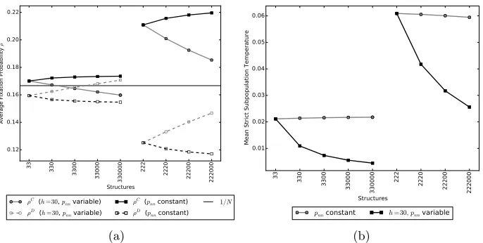
Figure 8: Figure (a) shows the effect of compensating for empty places by increasing the home fidelity such that the probability of staying in their home place,pnn, remains the same. We start ath = 30 for the 33 and 222 structures. As an empty place is added,h is increased so thatpnn= 30/31 for the 330,. . . ,330000 structures andpnn= 30/32 for 2220,. . . ,222000 structures. In all casesr= 30 andv= 10. We can see that after compensating for the above effect, the influence of introducing empty places is both reversed and weakened. Figure (b) shows the mean strict subpopulation temperature dropping off when we compensate for the empty places by increasing the home fidelity such thatpnnremains the same.
visit non home places and we therefore investigate what effect this has on the
454
evolution of cooperation.
455
As seen in Figure 4, increasing the number of empty places that
subpopu-456
lations can visit, whilst keeping all other parameters constant, makes it more
457
difficult for cooperation to evolve. In particular, this effect is prominent for
458
structures where cooperators were initially doing well. For example, for the
459
structure 222 where the cooperators do best, increasing the number of places
460
significantly reduces their fixation probability whilst increasing that of the
de-461
fectors. Here increasing the number of places acts in the same way as decreasing
462
the home fidelity, i.e. as decreasing the amount of time an individual spends in
463
its home place with members of its subpopulation. Thus the amount of time
464
an individual spends alone or with individuals not from its subpopulation
in-465
creases, so that the overall fitness of a cooperative subpopulation will decrease
466
(they still pay a cost but do not receive a benefit when alone). In terms of
467
the dynamics, spending more time alone would increase the effect of selection
468
in DBB dynamics because an individual with higher fitness that is randomly
469
chosen for death is more likely to be replaced by its own offspring, which affects
470
the cooperators adversely. A cooperative subpopulation will also have lower
471
fitness because its members are more likely to interact with individuals from
472
other subpopulations, therefore exposing them to defectors. The increased
in-473
teraction between individuals will also increase the effect of selection in DBB
474
dynamics because an individual with higher fitness that is randomly chosen for
death is less likely to be replaced by an individual with lower fitness in the same
476
subpopulation.
477
The increase in the number of places can be compensated for by increasing
478
the home fidelity, so that individuals stay in their home place with the same
479
probability. This has the effect of decreasing the mean strict subpopulation
480
temperature as individuals are more likely to spend time with members of their
481
subpopulation. This is shown in Figure 8, where we can see that the effect of
482
adding empty places is now reversed, although the strength of this reverse effect
483
is weak.
484
5.4. The effect of a large home fidelity 485
Consider a well-mixed population of M subpopulations each containing L
486
individuals, so that N = M L, as described in Section 2.3, where h is very
487
large. Consequently from equation (3.1),χ(m,G) is approximately 1 ifG=Qm, 488
and is approximately 0 otherwise. Thus the fitness of an individual can be
489
evaluated assuming that we have a group containing precisely all individuals
490
from its subpopulation with probability 1. Due to the symmetric nature of our
491
population, the weights for any two individuals in the same subpopulation will
492
be the same, as will the weights for any two members of different subpopulations.
493
Denoting the latter aswO, which will be small, we havewij=wO whenIi and 494
Ij are not in the same subpopulation, andwij =wI ≈[1−(M−1)LwO]/(L−1) 495
otherwise, with the probability of self-replacement negligible.
496
It follows that only replacements within subpopulations will happen, except
497
very rarely. Thus we can assume that the battle within any mixed subpopulation
498
of cooperator (C) and defector (D) individuals will be resolved with fixation of
499
one type or the other before any new mixed subpopulation appears.
500
We thus consider a two stage process. Firstly, a new mixed group appears.
501
This occurs rarely, through the invasion of a cooperator into a defector
subpop-502
ulation, or a defector into a cooperator subpopulation. Assuming that there are
503
currently MC(MD = M −MC) cooperator (defector) subpopulations, such a 504
transition happens with probability
505
pCI=
MD
M
MCLwOFL(C)
(L−1)wIFL(D) +O(wO)
(5.1)
506
of a cooperator into a defector subpopulation, or
507
pDI = MC
M
MDLwOFL(D)
(L−1)wIFL(C) +O(wO) (5.2) 508
of a defector into a cooperator subpopulation. The termsFL(C) andFL(D) are 509
the fitnesses of cooperator and defector individuals within their own
subpopu-510
lations, and are obtained directly from equations (2.4) and (2.6), and the terms
511
O(wO) are of the order ofwO, and very small. Further denotingx=v/[r(L−1)] 512
we obtain that the ratio of the two expressions in equations (5.1) and (5.2), and
513
thus the relative frequency that the new invasions happen, is thus
514
pCI
pDI
≈
F
L(C)
FL(D)
2
=
1 + v−1
r
2
≈(1 + (L−1)x)2 (5.3)
for largev andr.
516
The second process considers fixation within a well-mixed group of size L.
517
Following [23] we obtain the formula
518
xi=
1 +Pi−1
j=1
Qj
k=1δβkk
1 +PL−1
j=1
Qj
k=1βδkk
, (5.4)
519
for the fixation probability oficooperators within a population of sizeL. Here
520
βk (δk) is the probability that the next event is the replacement of a defector 521
(cooperator) by a cooperator (defector), when the number of cooperators isk.
522
We have here
523
δk =
k(L−k)
L
r+Lkv−1
(L−1)r+ ((L−k)k+ (k−1)2) v
L−1−(k−1)
, (5.5)
524
525
βk =
k(L−k)
L
r+(kL−−1)1v −1
(L−1)r+ ((L−k−1)k+k(k−1))Lv−1−k. (5.6)
526
For sufficiently larger, we obtain
527
δk
βk
≈ 1 +kx
1 + (k−1)xfk(x), (5.7)
528
where
529
fk(x) =
L−1 + (L−2)kx
L−1 + ((L−2)k+ 1)x <1. (5.8)
530
The fixation probability of a single cooperator in a group of defectors is given
531
by ρC,L = x1, and the fixation probability of a single defector in a group of
532
cooperators isρD,L= 1−xL−1. We thus have
533
ρD,L
ρC,L
=
L−1
Y
k=1
δk
βk
=
L−1
Y
k=1
1 +kx
1 + (k−1)xfk(x) = (1 + (L−1)x) L−1
Y
k=1
fk(x). (5.9) 534
535
This implies that
536
pCI
pDI
>ρD,L
ρC,L
. (5.10)
537
Following our assumptions, the population evolves following a succession of
538
invasions of subpopulations either of cooperators by defectors or of defectors by
539
cooperators. The probability that the next such event will be the invasion of a
540
subpopulation of defectors by a cooperator is simply
541
pCIρC,L
pCIρC,L+pDIρD,L
= rS 1 +rS
, (5.11)
542
where rS = pCIρC,L/pDIρD,L is the forward bias [40] of cooperative groups 543
within our population. For a cooperator to fixate in the population it must first
fixate within its group with probabilityρC,L, after which, there is a competition 545
between groups proceeding precisely as in a Moran process, so that we have
546
ρC=ρC,L
1−1/rS
1−(1/rS)M
, (5.12)
547
with the equivalent expression forρD, 548
ρD=ρD,LrS
−1
rM
S −1
. (5.13)
549
It is clear from equation (5.10) thatrS >1, so thatρC is greater thanρC,L(1− 550
1/rS) for anyM. LettingM become large means that 1/N= 1/M Lwill be less 551
thanρC, but larger than ρD, so that inequality (4.1) holds. This means that 552
for sufficiently largeh, r andv, we have that cooperation evolves for any given
553
subpopulation size L. Thus cooperation can potentially evolve for arbitrarily
554
large subpopulations, although as we have seen previously, it is easier for smaller
555
subpopulations.
556
6. Discussion 557
In [10] a new framework for the flexible modelling of structured populations
558
using multiplayer interactions was introduced, see also [8, 13, 11]. This work
559
built on classical evolutionary graph theory, but was limited in terms of the
560
dynamics used. In this paper we have developed this framework further. Most
561
importantly we have developed a full range of dynamics to apply in the
frame-562
work, which will allow us to consider many different evolutionary scenarios. In
563
particular these can be applied for the fully independent model in general, not
564
just the examples considered here, enabling us to use a fuller range of the
pos-565
sibilities that our flexible framework allows. Thus this paper can be thought to
566
complete the basic development phase of our work.
567
We have then developed the fully independent model to incorporate
subpop-568
ulations and in particular consider a generalized version of the territorial raider
569
model introduced in [8]. This is beneficial because previously the fully
inde-570
pendent model, represented in the bipartite graph in Figure 1, would require
571
a vertex for every individual as well as an additional vertex for every available
572
place. Now we just need a vertex per subpopulation, potentially allowing a
573
small number of very large subpopulations to be considered, which would not
574
have been possible previously. Furthermore, generalizing the territorial raider
575
model in this allows modelling of more complex movement behaviour as seen
576
in, for example, African wild dogs that live in packs [17].
577
This type of structure has been considered in a slightly different context,
578
for example, the island- or community-structured populations of [53]. In this
579
model interactions occur at multiple levels, interactions between community
580
members being more common than those with non-community members where
581
interaction occurs at multiple levels. Members of one community first play a
582
public goods game and then join the members of another community and play a
public goods game such that, at the highest level, the entire population plays a
584
public goods game. This is in contrast to our case, where individuals only play
585
a game if they are present in the same place at the same time. They showed
586
that cooperation can evolve when DBB dynamics are used and selection is weak
587
within communities, which is consistent with our results.
588
We note that the framework of [8] is capable of modelling far wider
be-589
haviour than that developed here, in particular it is able to consider dynamic
590
populations whose distributions continuously change due to their history, and
591
the interactions that they have. Thus it can incorporate the type of situations
592
with mobile populations modelled in [55, 47]. In particular, movement can
fol-593
low a stochastic process in which the individuals move depending upon their
594
current state as in [16]. In a soon to be recently submitted paper [39] we have
595
developed a Markov chain version of our model similar to this, and again
con-596
sider a combination of theoretical developments and the specific application of
597
the evolution of cooperation.
598
We then applied our new methodology to an example, considering the
evolu-599
tion of cooperation within a population involving subpopulations. We saw as in
600
evolutionary graph theory that the choice of dynamics is crucial, and that DBD
601
(and BDB) dynamics would not allow cooperation to evolve, but that DBB (and
602
BDD) would, which is consistent with [36]. Further, using the latter dynamics,
603
the size and the level of isolation of the subpopulations is important, with the
604
smaller the subpopulations and the greater the isolation, the greater the chance
605
for cooperation to evolve. Unsurprisingly, the larger the level of rewardv, the
606
better the cooperators do. In particular, the larger the subpopulations, the
607
larger the rewardvrequired for cooperation to evolve; note that this is similar
608
to the requirement that the benefit-to-cost ratio exceeds the average number of
609
neighbours an individual has from [36].
610
We see from Figure 6 that our new idea of strict subgroup temperature
611
is important in explaining the level of cooperation that evolves. Low (high)
612
temperature helps promote the invasion of cooperators (defectors). In
particu-613
lar, higher temperatures allow cooperators to cluster more strongly and benefit
614
more from cooperating with one another. We note that this raises a more
gen-615
eral question about temperature. Within subpopulation temperature includes
616
replacement weights between pairs of individuals from different subpopulations,
617
but excludes weights between pairs from within the same subpopulation. What
618
if two individuals have very similar, but not identical, movement distributions
619
(and thus whilst formally not within the same subpopulation, for practical
pur-620
poses they might as well be)? Under the current definition no distinction is made
621
between this and two individuals whose distributions are completely different.
622
We will investigate this question in later work.
Acknowledgments 624
This work was supported by funding from the European Union’s Horizon
625
2020 research and innovation programme under the Marie Sklodowska-Curie
626
grant agreement No 690817. The research was also supported by the Simons
627
Foundation Grant 245400 to JR and a City of London Corporation grant to KP.
628
References 629
[1] Allen, B. and Nowak, M. [2014], ‘Games on graphs’,EMS Surveys in Math-630
ematical Sciences 1(1), 113–151.
631
[2] Allen, B. and Tarnita, C. [2014], ‘Measures of success in a class of
evolu-632
tionary models with fixed population size and structure’,Journal of Math-633
ematical Biology68(1-2), 109–143.
634
[3] Antal, T. and Scheuring, I. [2006], ‘Fixation of strategies for an
evo-635
lutionary game in finite populations’, Bulletin of Mathematical Biology 636
68(8), 1923–1944.
637
[4] Archetti, M. and Scheuring, I. [2011], ‘Coexistence of cooperation and
de-638
fection in public goods games’, Evolution65(4), 1140–1148.
639
[5] Archetti, M. and Scheuring, I. [2012], ‘Review: Game theory of public
640
goods in one-shot social dilemmas without assortment’, Journal of Theo-641
retical Biology 299, 9–20.
642
[6] Binmore, K. [1992],Fun and Games: A Text on Game Theory, D.C. Heath.
643
[7] Broom, M., Cannings, C. and Vickers, G. [1997], ‘Multi-player matrix
644
games’,Bulletin of mathematical biology 59(5), 931–952.
645
[8] Broom, M., Lafaye, C., Pattni, K. and Rycht´aˇr, J. [2015], ‘A study of
646
the dynamics of multi-player games on small networks using territorial
647
interactions’, Journal of Mathematical Biologypp. 1–24.
648
[9] Broom, M. and Rycht´aˇr, J. [2008], ‘An analysis of the fixation
proba-649
bility of a mutant on special classes of non-directed graphs’, Proceedings 650
of the Royal Society A: Mathematical, Physical and Engineering Science 651
464(2098), 2609–2627.
652
[10] Broom, M. and Rycht´aˇr, J. [2012], ‘A general framework for analysing
653
multiplayer games in networks using territorial interactions as a case study’,
654
Journal of Theoretical Biology302, 70–80.
655
[11] Broom, M. and Rycht´aˇr, J. [2016], ‘Ideal cost-free distributions in
struc-656
tured populations for general payoff functions’, Dynamic Games and Ap-657
plications pp. 1–14.
[12] Broom, M. and Rycht´aˇr, J. [2013], Game-Theoretical Models in Biology,
659
CRC Press, Boca Raton, FL.
660
[13] Bruni, M., Broom, M. and Rycht´aˇr, J. [2014], ‘Analysing territorial models
661
on graphs’, Involve, a Journal of Mathematics7(2), 129–149.
662
[14] Bukowski, M. and Miekisz, J. [2004], ‘Evolutionary and asymptotic
sta-663
bility in symmetric multi-player games’, International Journal of Game 664
Theory33(1), 41–54.
665
[15] Domenici, P., Batty, R., Simil¨a, T. and Ogam, E. [2000], ‘Killer whales
666
(orcinus orca) feeding on schooling herring (clupea harengus) using
un-667
derwater tail-slaps: kinematic analyses of field observations’, Journal of 668
Experimental Biology203(2), 283–294.
669
[16] Erovenko, I. and Rycht´aˇr, J. [2016], ‘The evolution of cooperation in
one-670
dimensional mobile populations’,Far East Journal of Applied Mathematics 671
95(1), 63-8895(1), 63–88.
672
[17] Ginsberg, J. and Macdonald, D. [1990], Foxes, wolves, jackals, and dogs: 673
an action plan for the conservation of canids, IUNC, Gland, Switzerland.
674
[18] Gokhale, C. and Traulsen, A. [2010], ‘Evolutionary games in the
multi-675
verse’, Proceedings of the National Academy of Sciences 107(12), 5500–
676
5504.
677
[19] Gokhale, C. and Traulsen, A. [2014], ‘Evolutionary multiplayer games’,
678
Dynamic Games and Applicationspp. 1–21.
679
[20] Hamilton, W. [1967], ‘Extraordinary sex ratios’, Science156(3774), 477–
680
488.
681
[21] Harsanyi, J. and Selten, R. [1988], ‘A general theory of equilibrium selection
682
in games’,MIT Press Books1.
683
[22] Hauert, C., De Monte, S., Hofbauer, J. and Sigmund, K. [2002],
‘Volun-684
teering as red queen mechanism for cooperation in public goods games’,
685
Science296(5570), 1129–1132.
686
[23] Karlin, S. and Taylor, H. [1975], A First Course in Stochastic Processes,
687
London, Academic Press.
688
[24] Li, A., Broom, M., Du, J. and Wang, L. [2016], ‘Evolutionary dynamics of
689
general group interactions in structured populations’, Physical Review E 690
93(2), 022407.
691
[25] Li, A., Wu, B. and Wang, L. [2014], ‘Cooperation with both synergistic
692
and local interactions can be worse than each alone’,Scientific Reports 4.
693
[26] Lieberman, E., Hauert, C. and Nowak, M. [2005], ‘Evolutionary dynamics
694
on graphs’, Nature433(7023), 312–316.
![Figure 1: The fully independent model from [10]. There are Nmeet in individuals who are distributedover M places such that In visits place Pm with probability pnm](https://thumb-us.123doks.com/thumbv2/123dok_us/1425811.95235/4.612.173.441.123.241/figure-independent-nmeet-individuals-distributedover-places-visits-probability.webp)
![Figure 2: The territorial raider model of [10, 8]. (a) Population structure represented using agraph where vertices represent individuals and places](https://thumb-us.123doks.com/thumbv2/123dok_us/1425811.95235/7.612.164.446.404.504/figure-territorial-population-structure-represented-vertices-represent-individuals.webp)
![Table 2: Dynamics defined using the replacement weight as in [40]. In each case, B (D) isappended to the name of the dynamics if selection happens in the birth (death) event.](https://thumb-us.123doks.com/thumbv2/123dok_us/1425811.95235/10.612.138.476.124.230/table-dynamics-dened-replacement-isappended-dynamics-selection-happens.webp)