Modeling supersonic heated jet noise at fixed
jet
Mach number
using an asymptotic approach for the acoustic analogy Green’s
function and an optimized turbulence model
M. Z. Afsar∗
Department of Mechanical&Aerospace Engineering, University of Strathclyde, Glasgow, G1 I XJ
A. Sescu†
Department of Aerospace Engineering, Mississippi State University, Starkville, MS
E. Minisci‡
Department of Mechanical&Aerospace Engineering, University of Strathclyde, Glasgow, G1 I XJ
In this study we show how accurate jet noise predictions can be achieved within Goldstein’s generalized acoustic analogy formulation for heated and un-heated supersonic jets using a previously developed asymptotic theory for the adjoint vector Green’s function and a turbulence model whose independent parameters are determined using an optimization algorithm . In this approach, mean flow non-parallelism enters the lowest order dominant balance producing enhanced amplification at low frequencies, which we believe corresponds to the peak sound at small polar observation angles. The novel aspect of this paper is that we exploit both mean flow and turbulence structure from existent Large Eddy Simulations database of two axi-symmetric round jets at fixed jet Mach number and different nozzle temperature ratios to show (broadly speaking) the efficacy of the asymptotic approach. The empirical parameters that enter via local turbulence length scales within the algebraic-exponential turbulence model are determined by optimizing against near field turbulence data post-processed from the LES calculation. Our results indicate that accurate jet noise predictions are obtained with this approach up to a Strouhal number of0.5for both jets without introducing significant empiricism.
I. Introduction
A
eroacoustic modeling of jet noise within Goldstein’s generalized acoustic analogy (GAA)[1] formulation involves(a) solving the adjoint linearized Euler equations to determine the Green’s function that defines the so-called propagator tensor and (b) appropriately modeling the Reynolds stress auto-covariance using experimental data and/or numerical simulations [1]. The far-field sound is then determined by the volume integral of an inner product of the propagator and the Reynolds stress auto-covariance tensors. This approach has proven to be successful for a number of test cases involving axi-symmetric round jets at a variety of acoustic Mach numbers and observation angles, Goldstein & Leib [2] (hereafter referred to as G&L) and [3]). It has also shed light on what impact the mean flow field has on the far-field radiated sound for both heated and unheated flows [4].G&L’s predictions were computed atO(1) (i.e., arbitrary) frequencies for a propagator tensor based on a weakly non-parallel mean flow. Non-parallelism appeared in the analysis at supersonic speeds and only affected the solution within a thin critical layer where the adjoint vector Green’s function is singular for the locally parallel mean flow. G&L constructed a uniformly valid composite solution for the adjoint Green’s function, thus eliminating the critical-layer singularity that occurs when the observation angle,θ, is close to the downstream jet axis. They showed that, asθ→0, the dominant contribution to the propagator comes from the radial derivative of the Fourier transformed adjoint Green’s function for the streamwise momentum perturbation. This was also confirmed by Karabasov et al. [5]’s numerical calculations and by Afsar et al. [3] who, together with G&L, showed that the acoustic efficiently of this term is raised to a dipole at low frequencies even though it appears as a quadrupole when multiplied by the appropriate Reynolds stress auto-covariance component in the acoustic spectrum formula [6].
∗
Chancellor’s Fellow. AIAA Member.
†
Associate Professor, and AIAA Associate Fellow.
‡
Experimental [13] LES case Description Mj T R Ma
B118 A1 isothermal ideally-expanded 1.5 1.0 1.5
B122 A2 heated ideally-expanded 1.5 1.74 1.98
Table 1 Br`es et al (2012) [12] test cases
Physically, this behavior is due to the streamwise-radial, or ‘1-2’, component of the fluctuating Reynolds stress multiplying the commensurate propagator component in such a manner that the latter possesses a pre-factor with directionality that scales as cos4θ/(1−M(r)cosθ)6(whereM(r)is the local Mach number profile), which, obviously, peaks asθ → 0 (whereθis the polar observation angle), thus allowing an accurate prediction to be made of the peak jet noise that experiments show usually occurs atθ =30o in the forward arc. This result was derived in the matched-asymptotic-expansion sense, in which the solution for the pressure-like Green’s function is divided into an inner region where the scaled radial coordinater/σ=O(1)and anr =O(1)outer region with the scaled frequency,
σ=k∗∞δ∗O(1), being an asymptotically small parameter everywhere in the flow (δ∗is an appropriate dimensional length scale such as the nozzle radius andk∞is far-field wavenumber). Parallel flow asymptotics also showed that the components of the fluctuating Reynolds stress (other than ‘1-2’) make a more dominant contribution to the large-angle-radiated sound atO(1) frequencies under a general axi-symmetric representation of the Reynolds stress auto-covariance tensor (such as that in [7]). This picture of jet noise is, however, oversimplified because it does not take into account mean flow spreading, which Karabasov et al. [8] showed can be important atO(1) Mach numbers and can increase the low-frequency radiation by as much as 8 Decibels (dB) forθ=30oon a subsonic jet compared to the equivalent parallel flow solution of the GAA (adjoint linearized Euler) equations.
Goldstein, Sescu & Afsar [9] (referred to herein as GSA) constructed an asymptotic solution to the adjoint vector Green’s function problem starting from the GAA equations. As opposed to low-frequency asymptotics in a parallel flow discussed above, they considered a slowly diverging jet flow in which the spread rate,, is an asymptotically small parameter, O(1). GSA determined that the only distinguished limit that could produce leading order changes to the acoustic spectrum is when the Strouhal number is of the same order as the jet spread rate. The resulting adjoint vector Green’s function (and therefore the dominant ‘1-2’ propagator component mentioned above) was different from the parallel flow result everywhere in the jet (not just in the critical layer as in [2]). Following on from GSA, Afsar et al. [10] assessed the predictive capability of the asymptotics by using Reynolds-averaged Navier-Stokes (RANS) mean flow solutions to calculate the adjoint Green’s function and the low-frequency asymptotically dominant propagator term in the GAA equations. Their main numerical result (figure 5.3a) confirms that an accurate prediction of the far-field sound at low Strouhal number can be made using this asymptotic approach. The predictions generally break down (i.e., rapidly decrease), however, above the peak Strouhal number (at St=0.3 or so), but that is not altogether unexpected owing to low-frequency applicability of the theory.
In this paper our aim is to further investigate the applicability of the non-parallel flow asymptotic approach by considering the effect of heating and supersonic flow using a large-eddy simulations (LES) database of two axi-symmetric round jets at a fixedjetMach number ofMj =1.5. These solutions were reported in [11] (see also [12]) and identified by the designations B118 and B122 for the unheated and heated configurations, respectively. The operating conditions are summarized in Table 1. As opposed to our previous studies ([10] & [14]) however, the novel aspect of this paper is that the parameters of the turbulence model for the ‘1212’ component of the Reynolds stress auto-covariance tensor that enters the acoustic spectrum formula for the peak sound are optimized using near field turbulence data post-processed from the LES data of [12]. In this manner the model for jet noise requires only very minimal aposteriori empirical tuning. The predictions, in general, remain with(1−2)dB of the acoustic data up to a Strouhal number of about 0.6 for both jets. Since the turbulence model that we use (prior to optimization) for the Reynolds stress auto-covariance tensor is the only unknown here, this approach also highlights what aspects of that model can be improved upon in order to obtain better agreement with the acoustic data.
II. Summary of asymptotic approach
Suppose that all lengths have been normalized by the nozzle radius,Dj/2, and all velocities by the mean jet exit velocity,Uj. Let the pressurep, densityρ, enthalpyh, and speed of soundcsatisfy the ideal gas law equation of state p=ρc2/γ
the low-frequency acoustic spectrum at the observation point,x=(x1,xT)=(x1,x2,x3), due to momentum and energy
transfer (via temperature fluctuations) symbolized by the generalized stress tensoreλj(y, τ)=[ρv0λv0j−ρvλ0v0j](y, τ)in the acoustic spectrum formula, where turbulence is contained within a volumeV(y), is given by
I(x,y;ω) ≈
2c2∞|x| 2
4|G12|2+(3−γ)n2Re
Γ41G∗
11 +n3|Γ41|2
Φ∗
1212 (1)
that is related to the Fourier transform of the far-field pressure auto-covariance,p0(x,t)p0(x,t+τ)by
I(x;ω)=
∫
V∞(y)
I(x,y;ω)dy, (2)
where|x| → ∞andp0(y, τ) ≡p(y, τ) −p(¯ y). As usual, over-bars are being used to denote time averages defined by:
¯
•(x) ≡ lim T→∞ 1 T T ∫ 0
•(x,t)dt, (3)
where•in (3) is a place holder for any fluid mechanical variable.
In the acoustic spectrum integral (2), cylindrical polar coordinates y = (y1,r, ψ), commensurate with an
axi-symmetric round jet, are defined with respect to an origin at the nozzle exit plane. We allow normalized co-variance components, R4111 =n2R1212 andR4141 =n3R1212 where(n2,n3)areO(1)constants and suffix ‘4
0
indicates static enthalpy fluctuation viav04 :=(γ−1)(h0+v02/2) ≡ (c2)0+(γ−1)v02/2 whereh0is the fluctuating static enthalpy and(c2)0is the fluctuations in the sound speed squared such thatv04/(γ−1)denotes the moving frame stagnation enthalpy fluctuation [1]. Equation (1) will continue to hold for isothermal jets when mean flow quantities and turbulence parameters are appropriately defined (i.e. temperature associated correlation functions are zero: n2 =n3=0).
A. The propagator solution
The Fourier transformed adjoint Green’s functions (G¯1,G¯4)represent the Green’s function for the streamwise
linearized momentum and energy equations of the generalized acoustic analogy ([1] & [14]); they enter (1) through the propagator components:
G12=G˜12(Y,U)= ∂G˜1
∂r − (γ−1)G˜4
∂U
∂r (4)
and, similarly,
G11=G¯11(Y,U)=
∂G¯ 1
∂Y − (γ−1)G¯4
∂U
∂Y
& Γ41=Γ¯41(Y,U)= ∂G¯1
∂Y (5)
that are determined for the Favre-averaged mean flowv˜ = ρv/ρ¯ =(U,Vr)(y)that depends ony1 through the slow
streamwise coordinateY =y1=O(1)for a jet of an asymptotically small spread rate,O(1). The mean flow then
divides into an inner region given by slowly varying mean flow expansion formulae, equations (13) –(17) in [15] (or,
equations 3.1-3.4 in GSA), wherer=|yT|=
q y2
2+y 2
3 =O(1), and an outer region at radial distances,R=r=O(1).
The propagator component ˜G12(y;Ω)is then defined at the particular scaled temporal frequency,Ω=ω/ =O(1),
shown by GSA to be where mean flow non-parallelism changes the lowest-order structure of the adjoint Green’s function solution(G¯1,G¯4)everywhere in the flow (and not just in the critical layer at supersonic speeds as in G&L’s solution) and
atO(1)Mach numbers. This distinguished limit follows supposing that the space-time adjoint vector Green’s function,
ga
ν4(y, τ|x,t), depends on time,τ, through theO(1)slowly breathing time ˜T =τwhere suffixν=1,2..5 corresponding
to the 5 linearized Euler equations of the generalized acoustic analogy in [1]. In other words, as pointed out in our earlier paper [9], the Strouhal number,St, is of the order of the jet spread rate,, in the solution of Fourier transform of
gaν
4(y, τ|x,t)(Eqs. 7–9 in [10]).
The asymptotic structure of the adjoint Green’s function(G¯1,G¯4)is then identical to the mean flow in that it also
ofgνa4(y, τ|x,t)forν =(1,4)(see below 6∗) and corresponds to the zeroth order azimuthal mode expansion since higher-order modes produce an asymptotically small (i.e.,O()) correction to the lowest order and therefore can be neglected atO(Ω0).
[9] showed how tremendous simplification can be achieved by taking(Y,U)rather than(Y,r)as the independent variables of choice. The implicit function theorem shows thaty=(Y,r)can be implicitly related to the field space y=(Y,U(Y,r))and that the Green’s function variable ˜Gi(y|x;Ω)=(G˜1,G˜4)(y|x;Ω)then depends on(y;Ω)through
field space(Y,U(Y,r);Ω) ≡ (Y,r;Ω). The one-to-one transformation of independent variables,(Y,r) → (Y,U), can be used together with the chain rule to combine the appropriate inner equations (19-21 in [10]) to the second-order hyperbolic partial differential equation
e
c2 ∂ ∂U 1 e c2 ¯ D0ν¯
+X¯1∂
2ν¯
∂U2 =0, (6)
in whichY = const.,dU/dY = X˜1/U are characteristic curves ([16], pp. 121-122). This equation requires that
e
c2(Y,r)= f(U)and satisfies Crocco’s relation, and for the scaled composite Green’s function variable ¯ν=ce2G¯4+G¯5
(Eq. 18 in [10]) where ¯G5 corresponds to the Fourier transform of the scaled Green’s function for the linearized
continuity equation (Eq. 2.22a in [1]). But the Crocco-Busemann relation (see equation 2.4c in [17]), which applies when the jet flow is heated, shows that the mean speed of sound is still a function ofU(Y,r). Therefore, Eq.(6) will continue to hold in such a case. The advantage of solving this equation to determine the low-frequency structure of the adjoint linearized Euler equations (equations 4.8 - 4.10 of [2]) is clear. The hyperbolic structure of equation (6) shows that it is unnecessary to impose a downstream boundary condition. Figure 1 in [9] indicates how information propagates to both the left and the right from theU=0 boundary and that no boundary conditions are required on theY =0 and Y → ∞boundaries (i.e., no inflow boundary condition is required here). Hence the solution for the composite variable
ν(Y,U)is now uniquely determined by the outer boundary conditions (i.e., by matching to the inner limit of the outer solution using Van Dyke’s rule [18])
¯
ν(Y,0) → −iΩc2 ∞e
−iΩYcosθ/c∞
(7)
∂ν¯
∂U(Y,0) → −iΩc∞cosθe
−iΩYcosθ/c∞
(8)
on the non-characteristic curveU =0, withY ≥0 (where, as indicated above,U → 0 corresponds to outer limit, r→ ∞). The coefficient ¯X1is the streamwise component of the mean flow advection vector (equation 5.15 in [9]) and
¯
D0 =iΩ+U∂/∂Y.
The inner solutionν(Y,U)is then induced by incoming waves by the outer wave equation. For theO(Ω0)solution, any influence of the nozzle (i.e., via the scattered wave contribution to the outer solution) can be neglected because the inner solution, which generates the scattered waves, will not behave logarithmically asr → ∞when matched to the outer solution. The logarithmic behavior of the axi-symmetric mode of the scattered solution (5.2 in [9]) follows from the small argument expansion for the solution to the two-dimensional Helmholtz equation ([19], p. 891) in the outer region. Using Van Dyke’s rule, this expansion shows thatν(0,Y)will not match onto the transcendental lnRbehavior which the solution to the Helmholtz equation induces when the inner limit is taken; i.e. asR→0 in the outer region at O(Ω0)frequencies.
B. Turbulence modeling
The turbulence enters the acoustic spectrum formula (1) through the spectral tensor componentΦ1212(y;ω)defined
by the space-time Fourier transform
Φ1212(y;ω)= 1 2π
∫
V(η)
∫ ∞
−∞
R1212(y,η;τ)ei(k.η−ωτ)dηdτ, (9)
where theR1212(y,η;τ)component of the Reynolds stress auto-covariance tensor is given by the time-average
R1212(y,η;τ)= lim T→∞ 1 2T ∫ T −T h ρv0
1v 0 2−ρv
0 1v
0 2 i
(y, τ)hρv0 1v
0 2−ρv
0 1v
0 2 i
(y+η, τ+τ0)dτ0. (10)
∗
The re-scaling of Fourier transform ofgνa4(y, τ|x,t)via Eq. 18 in [10] for(G¯1,G¯4),G¯5), which enter either the composite solution
¯
ν=fc2G¯
Construction of R1212(y,η;τ) using an exponential model with algebraic tails and the subsequent calculation of
Φ1212(y;ω)is worked out in [10], and we use their final result
Φ1212(y;ω)=2πA1212(y) l
0l1l2⊥ χ2U
c
× (11)
(1−a1−a2)+(a1ω˜2−k¯
1(ω˜(a1−a2)(l1/l0) −a1k¯1))(4/χ)
where χ(ω,˜ k¯1)=k¯12+ω˜2+1=(k1−ω˜(l1/l0))2+ω˜2+1 and ˜ω =(ωl0/Uc)is the normalized temporal frequency
whereUcis the convection velocity of the turbulence (fixed atUC =0.68 following experiments by Harper-Bourne). The length scales in Eq. (11) are taken to be proportional to the local turbulent kinetic energyk(y)and the rate of energy dissipation ˜(y)asli(y)=ci(k3/2/˜)(y)fori =0,1,2,3. We scale the amplitude ofR1212(y,η;τ)as follows:
R1212(y,0; 0)=a1212ρ¯2(y)k2(y)where ¯ρ(y)k(y)is the density-weighted RANS turbulent kinetic energy (TKE).a1212
is usually approximated by its (maximum) value on the shear layer locationr=0.5 at the end of the potential core of the jet ([5]). Since [14] show thatR1212(y,η;τ)depends on the 5 parametersl1/l0=c1/c0,c⊥,a1,a2anda1212that we
obtain (together with mean flow) from the LES data rather than scaling a RANS mean flow as done by [5]. For example, we show in section§.(III) thata1212remains largely constant in the jet. The parameters in Eq. 11: namely, length scale
ratio(c1/c0)and anti-correlation parameters(a1,a2)are determined by using an adaptive algorithm (MP-AIDEA) to
determine their optimum values against post-processed data from the LES calculations reported in [12].
Multi Population Adaptive Inflationary Differential Evolution Algorithm (MP-AIDEA, [20] & [21]) is a population-based evolutionary algorithm for solving single-objective global optimisation problems over continuous spaces. It combines adaptive Differential Evolution (DE) with the restarting procedure of Monotonic Basin Hopping (MBH) ([22] &[23]). Multiple populations are initialised in the search space and exchange information during the optimisation process. Each population starts the search for the global minimum by running a DE algorithm. The user is not required to set the parameters of the DE, a process that could be extremely time consuming, since the best settings of the parameters are problem-dependent ([24] & [25]). Instead, MP-AIDEA is able to automatically adapt these parameters during the optimisation process. At the end of the DE a local search is run from the best individual of each population. Using the restarting mechanism of MBH in combination with the DE, the populations are able move, in a funnel structure, from one local minima to another, until the global minimum of the problem is located. MP-AIDEA implements a novel approach to avoid multiple detection of the same local minima, by restarting the population in the entire work space when it falls within the basin of attraction of an already detected minimum. The only element of empiricism in the noise predictions, however, is in the estimation ofc⊥that we did not analyze using the optimization algorithm. Its value, although varied by hand, turned out to be an order of magnitude smaller thanc1(the streamwise length scale parameter),
which is consistent with an axi-symmetric turbulence approximation used in this paper and analyzed more fully in [14].
III. Optimized turbulence correlations and SPL predictions
A. Mean flow development
The development of the mean flow components(U,Vr)in Fig. (1) shows how heating at fixed Mj reduces the potential core length (Figs. 11(a) & 1(d)) which is indicative of faster jet spreading. But we also see an increase in the magnitude ofX1(y1,r)=X¯1(Y,U)=Vr∂U/∂ralong the shear layer of the jet. By measuring the slope of the upper
most level curve of the streamwise mean flow in Fig. (11(a)) we estimate the jet spread rates to beB118=0.12 and B122 =0.15.
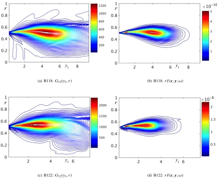
Figure 2 shows the contours of|G12|at the peak Strouhal number ofSt=0.2 and downstream observation angle
ofθ=300for the B118 (Figs.2(a) & 2(b)) and B122 (2(c) & 2(d)) jets. The convergence of the numerical algorithm applied to inner equation (6) has been analyzed in several of our previous papers (see [10] & [14]), and it was found to be within 5% at almost all regions of the jet, with only slight differences in∂ν¯/∂Ucoming near the inner boundary asU '0.7. The verification of the Crocco and Crocco-Busemann relations for B118 and B122 jets has also been performed in our paper [14] and found to be within 5% at worst.
The peak in the momentum flux propagator,|G12|, extends near the nozzle lip line peaking downstream aty1∼5−6
compared to the subsonic jet mean flow in [10]. The reason for this is that at supersonic speeds, non-parallelism at suppresses|G12|from becoming singular in the critical layer atΩ=O(1)frequencies. Note that extracting the centerline
streamwise velocity contourU(y1,0)in Fig.1(a) shows that the potential core lengths correspond to a streamwise length
(a) Streamwise mean flow,U(y1,r) (b) Radial mean flow,Vr(y1,r)
(c) Stremwise mean flow advection, ¯X1(y1,r) (d) Turbulent kinetic energy, ¯ρk(y1,r)
Fig. 1 Mean flow development for B118and B122jets.
|G12|to lie within one potential core length of the jet (cf. Figs.2(a) & 2(c)). In Figs. 2(b) & 2(d) shows contour plots of
the radius-weighted acoustic spectrumr ILOWusing one set of optimized scales for(lr,a1,a2)that shall be discussed
soon. The indication here is that the peak noise source lies just beyond the end of the potential cores of both jets (cf. streamwise potential core lengths above) such that the maximum contour level ofr I(x,y;ω)is greater with heating at fixedMj. While, at its greatest, this stands at an almost 2 order of magnitude increase inr I(x,y;ω)of 10−8(Fig.2(b)) compared to 10−10for B118 (Fig.2(d)), this intense region in B122 is much thinner inrand more localized within the potential core iny1 in Fig. (2(d)), hence it is likely that the surrounding (more blue) contours wherer I(x,y;ω)
∼(0.2-0.3)×10−8
[image:6.612.84.531.82.423.2]contribute more significantly to (2). This is then consistent with the almost 5−6dB increase in sound for these jets that the noise measurements of [26] indicate.
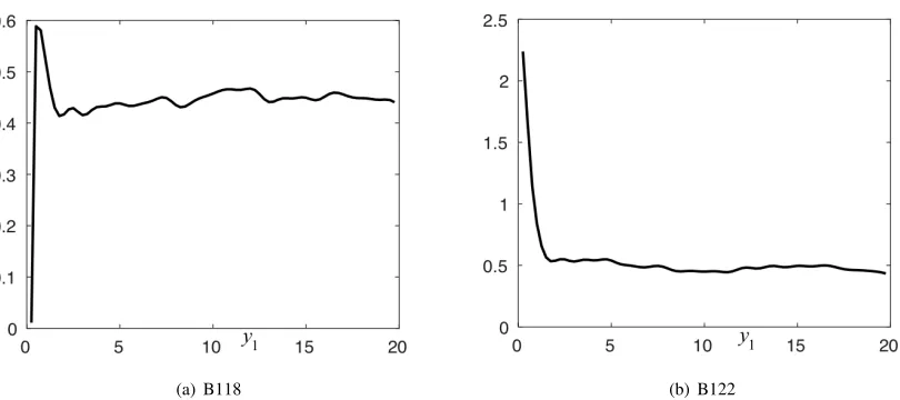
Figure 3 shows that LES extracted ratio R1212(y,0; 0)/ρ¯2(y)k2(y)=a1212determined at the shear layerr =0.5
remains more-or-less constant in the jet. Hence we fixa1212=0.45 for B118 anda1212=0.5 for B122. Figure 4 shows
the outcome of optimizing(lr,a1,a2)in:
R1212(y, η1,0, τ) R1212(y,0,0) =
1+a1
˜
τ
Xl
2
r(η˜1−τ˜) −a2
˜
η1
X[η˜1+l
2
r(η˜1−τ˜)]+...
e−X
(12)
where X=X(η˜1,η˜T,τ¯)= q
˜
η2 1+|ξ˜|
2, ˜η
(a) B118:G12(y1,r) (b) B118:r I(x,y;ω)
(c) B122:G12(y1,r) (d) B122:r I(x,y;ω)
Fig. 2 Spatial structure of momentum flux propagatorG12(y1,r), (4), and radius-weighted acoustic spectrum r I(x,y;ω), (1), for B118and B122jets.
only through the scaled non-dimensional convected variable, ˜ξ=lr(η˜1−τ¯)wherelr =l1/l0 =c1/c0.
We applied the MP-AIDEA algorithm in two ways. First by optimizing theR1212(y, η1,0, τ)model, (12), at all
˜
η1 =(0.0,0.3,0.6)(case a) and then at ˜η1 =0.0 only (case b). The results in Figure 4 indicate that whilst case b guarantees perfect agreement at ˜η1 =0.0 (Figs. 4(b) & 4(d)) it introduces a departure at ˜η1=(0.3,0.6). On the other
hand, for case a, (12) gets the right maximum height fromτ=0 axis, but the location of the peaks are shifted. But the acoustic predictions using these set of parameters for casesa&bdo not result in significant change for B118 (Fig.5(a)) and a difference of(1−3)dB for B122 (Fig.5(b)). Note that just as in the jet noise calculations in Afsaret al. (2019), we show in the appendix that a heated jet at fixedMj displays predictions for the peak sound that are more-or-less independent of(n2,n3)in (1). The B122 predictions in Figs. 5 & 6 are therefore taken at(n2,n3)=0. Given the fact
the caseboptimized parameters forR1212(y, η1,0, τ)where in agreement with caseafor the 300prediction in Fig.5,
we concentrate on this choice of parameters in Fig. 6. Here we show the predictions at various downstream angles
[image:7.612.85.521.89.450.2](a) B118 (b) B122
Fig. 3 Streamwise development ofR1212(y,0; 0)/ρ¯2(y)k2(y)atr=0.5for B118and B122jets.
Jet Optimization case lr a1 a2 c0 c1 c⊥
B118 a 0.56 0.37 1.0 0.3 0.176 0.075
B118 b 0.53 0.36 1.29 0.35 0.184 0.1
B122 a 0.432 0.277 1.0 0.3 0.130 0.034
[image:8.612.101.506.76.256.2]B122 b 0.965 0.0 0.688 0.3 0.289 0.017
Table 2 Optimized turbulence scales used in prediction via (12), (11), (1)&(2)
IV. Conclusion
The use of a nearly optimized turbulence model for the appropriate Reynolds stress auto-covariance tensor component R1212(y,η;τ)that enters the peak noise formula (1) results in acoustic predictions that are very accurate beyond what would normally constitute the low frequency regime. Our results show the robustness of the asymptotic approximation for the adjoint vector Green’s function of the linearized Euler equations in the presence of slowly diverging mean flow worked out by Goldstein-Sescu-Afsar [9] and re-formulated in [14]. In this paper we have extended the work of [10] and [14] to assess the validity of this approach for axi-symmetric flows of fixed jet Mach number. Our results have shown that the theory not only provides a means to understand, qualitatively, the effects of non-parallelism within the acoustic analogy but also provides excellent predictive capability of the jet noise. The reduced form of the acoustic spectrum formula (equation 19 in [4]) used here is limited to low frequencies and shallow downstream observation angles from the jet axis. The results in this paper indicate that the 30◦spectrum can be accurately predicted in both the unheated (B118) and heated (B122) cases up to a Strouhal number of almost 0.5. Future work will involve investigating different optimization techniques to better modelR1212auto-covariance.
Acknowledgments
(a) B118: case a (optimizing at allη1) (b) B118: case b ((optimizing atη1=0))
(c) B122: case a (d) B122: case b
Fig. 4 Application of MP-AIDEA algorithm to optimization of R1212(y, η1,0, τ)using (12) against LES data [12].
Appendix A: Effect of
n
2=
n
3,
0
in (1)
In Fig.(7) we show the effect on the peak acoustic spectrum of takingn2 =n3,0 in (1). As in the fixed acoustic
Mach number heated jet predictions in [14], our results show little (if any) sensitivity to(n2,n3)parameters in the
acoustic spectrum formula (1).
References
[1] Goldstein, M. E., “A generalized acoustic analogy.”J. Fluid Mech., Vol. 488, 2003, pp. 315–333.
[2] Goldstein, M. E., and Leib, S. J., “The aero-acoustics of slowly diverging supersonic jets.”J. Fluid Mech., Vol. 600, 2008, pp. 291–337.
[3] Afsar, M. Z., “Asymptotic properties of the overall sound pressure level of sub-sonic air jets using isotropy as a paradigm,”J. Fluid Mech., Vol. 8, No. 2, 1997, pp. 13–19.
[4] Afsar, M. Z., Goldstein, M. E., and Fagan, A. M., “Enthalpy-flux/momentum-flux coupling in the acoustic spectrum of heated jets,”AIAA J, Vol. 49, 2011, pp. 2252–2262.
[image:9.612.102.511.76.445.2](a) B118 (b) B122
Fig. 5 SPL prediction against acoustic data in [26]. SPL computed viaSPL =10log104π(ρU2J)2I(x;ω)/Pr e f2
where Pr e f =2×10⁻⁵ Pa. The spectrum I(x;ω)is determined by integrating (1) over y = (y1, r, φ) where
turbulence scales inΦ∗
1212(y,k1,k 2
T;ω), (11) summarized in table 2
[6] Goldstein, M. E., “The low frequency sound from multipole sources in axysymmetric shear flows with application to jet noise.” J. Fluid Mech., Vol. 70, 1975, pp. 595–604.
[7] Afsar, M. Z., “Insight into the two-source structure of the jet noise spectrum using a generalized shell model of turbulence.” Euro. J. Mech. B/Fluids, Vol. 31, 2012, pp. 129–139.
[8] Karabasov, S. A., Bogey, C., and Hynes., “Computation of noise of initially laminar jets using a statistical approach for the acoustic analogy: application and discussion,”AIAA 2011-2929, 2011.
[9] Goldstein, M. E., Sescu, A., and Leib, S. J., “Effect of non-parallel mean flow on the Green’s function for predicting the low frequency sound from turbulent air jets.”J. Fluid Mech., Vol. 695, 2012, pp. 199–234.
[10] Afsar, M. Z., Sescu, A., and Leib, S. J., “Predictive capability of low frequency jet noise using an asymptotic theory for the adjoint vector Green’s function in non-parallel flow,”AIAA Paper, Vol. 2016-2804, 2016.
[11] Br`es, G. A., Nichols, J. W., Lele, S. K., , and Ham, F., “Towards best practices for jet noise predictions with unstructured large eddy simulations,”AIAA Paper 2012-2965, 2012.
[12] Br`es, G., Ham, F., Nichols, J., and Lele, S., “Unstructured large eddy simulations of supersonic jets,”AIAA J, 2016.
[13] Schlinker, R. H., Simonich, J. C., Reba, R. A., Colonius, T., Gudmundsson, K., and Ladeinde, F., “Supersonic Jet Noise from Round and Chevron Nozzles: Experimental Studies,”AIAA 2009-3257, 2009.
[14] Afsar, M. Z., Sescu, A., and Sassanis, V., “Validity of a non-parallel flow asymptotic theory for the adjoint Green’s function within the generalized acoustic analogy: its role in explaining the ’quietening’ of heated supersonic jets,”Submitted to Phys. Fluids, 2019.
[15] Afsar, M. Z., Sescu, A., and Leib, S. J., “Predictive Capability of Low Frequency Jet Noise using an Asymptotic Theory for the Adjoint Vector Green’s Function in Non-parallel Flow,”AIAA 2016-2804, 2016.
[16] Garabedian, P. R.,Partial Differential Equations, AMS Chelsea Publishing, New York, 2008.
[17] Leesshafft, L., Huerre, P., Sagaut, P., and Terracol, M., “Nonlinear global modes in hot jets.”J. Fluid Mech., Vol. 554, 2006, pp. 393–409.
[18] Van Dyke, M.,Perturbation Methods in Fluid Mechanics, Parabolic Press, Stanford Univ., 1975.
[image:10.612.110.506.77.257.2][20] Di Carlo, M., Vasile, M., and Minisci, E., “Multi-Population Adaptive Inflationary Differential Evolution Algorithm with Adaptive Local Restart,”IEEE Congress on Evolutionary Computation CEC, Sendai, Japan, 2015.
[21] Di Carlo, M., Vasile, M., and Minisci, E., “Multi-Population Adaptive Inflationary Differential Evolution Algorithm,”BIOMA (Bio-Inspired Optimisation Methods and their Applications) Workshop, Ljubljana, Slovenia, 2014.
[22] Wales, D. J., and Doye, J. P. K., “Global optimization by basin-hopping and the lowest energy structures of Lennard-Jones clusters containing up to 110 atoms,”J. Phys. Chem. A, Vol. 101, 1997, pp. 5111–5116.
[23] Addis, B., Locatelli, M., and Schoen, F., “Local optima smoothing for global optimization,”Optimization Methods and Software, Vol. 20, 2005, p. 4170437.
[24] Minisci, E., and Vasile, M., “Adaptive Inflationary Differential Evolution,”IEEE Congress on Evolutionary Computation CEC, Sendai, Japan, 2014.
[25] Vasile, M., Minisci, E., and Locatelli, M., “An inflationary differential evolution algorithm for space trajectory optimization,” IEEE Transactions on Evolutionary Computation, Vol. 15 (2), 2011, pp. 267–281.
(a) B118:θ=300 (b) B118:θ=350
(c) B118:θ=400 (d) B122:θ=300
(e) B122:θ=350 (f) B122:θ=400
Fig. 6 SPL prediction against acoustic data in [26]. SPL computed as caption as Fig. (5). Turbulence scales inΦ∗
1212(y,k1,k 2
[image:12.612.97.520.92.661.2](a) Case a optimized parameters in (12) (b) Case b
Fig. 7 30degree prediction for B122jet against acoustic data in [26]. SPL computed as in Fig. (5). Turbulence scales inΦ∗
1212(y,k1,k 2
[image:13.612.94.517.289.467.2]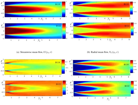
![Fig. 4Application of MP-AIDEA algorithm to optimization of R1212(y, η1, 0, τ) using (12) against LES data[12].](https://thumb-us.123doks.com/thumbv2/123dok_us/1328741.86775/9.612.102.511.76.445/fig-application-aidea-algorithm-optimization-using-les-data.webp)
![Fig. 5SPL prediction against acoustic data in [26]. SPL computed viawhere SPL = 10log104π(ρU2J)2I(x; ω)/P2ref Pref = 2 × 10⁻⁵ Pa](https://thumb-us.123doks.com/thumbv2/123dok_us/1328741.86775/10.612.110.506.77.257/fig-prediction-acoustic-data-spl-computed-viawhere-pref.webp)
![Fig. 6SPL prediction against acoustic data in [26]. SPL computed as caption as Fig. (5)](https://thumb-us.123doks.com/thumbv2/123dok_us/1328741.86775/12.612.97.520.92.661/fig-spl-prediction-acoustic-data-spl-computed-caption.webp)
![Fig. 730 degree prediction for B122 jet against acoustic data in [26]. SPL computed as in Fig](https://thumb-us.123doks.com/thumbv2/123dok_us/1328741.86775/13.612.94.517.289.467/fig-degree-prediction-acoustic-data-spl-computed-fig.webp)
