Simulation-based optimisation of LCC-HVDC controller parameters using surrogate model solvers

(1)

Simulation-based Optimisation of

LCC-HVDC Controller Parameters using

Surrogate Model Solvers

Aaron S. C. Leavy and Lie Xu

Department of Electronic and Electrical Engineering University of Strathclyde

Glasgow, United Kingdom {aaron.leavy, lie.xu}@strath.ac.uk

Shaahin Filizadeh and Aniruddha M. Gole

Department of Electrical and Computer Engineering

University of Manitoba Winnipeg, Canada

{shaahin.filizadeh, aniruddha.gole}@umanitoba.ca

Abstract—This paper proposes the use of surrogate model optimisation methods to solve box constrained LCC-HVDC controller tuning problems. The tuning problem is the selection of the proportional-integral controller gains and voltage-dependant current order limiter parameters of an LCC-HVDC link subject to two operational scenarios and a set of large-signal disturbances. The solvers using recently proposed surrogate model methods performed either similarly to or significantly better than solvers using mature methods of the types found in PSCAD/EMTDC, thus confirming the suitability of these surrogate model solvers for simulation-based optimisation of LCC-HVDC controllers.

Index Terms—Controller tuning, expensive black-box optimisation, LCC-HVDC, parameter selection, simulation-based optimisation.

I. INTRODUCTION

Prudent design and operation of LCC-HVDC schemes requires careful selection of controller parameters, including: proportional-integral (PI) controller gains; and voltage-dependant current order limiter (VDCOL) parameters. These parameters strongly influence the dynamic behaviour of HVDC schemes subjected to disturbances and set-point changes, and therefore affect the in-service satisfactory performance of those HVDC schemes.

Two feasible approaches to tuning these PI and VDCOL parameters are: optimal control techniques using linearised state-space models; or manual tuning via trail-and-error to find feasible solutions. However linearised models cannot explicitly model practical non-linear behaviours such as short-circuit faults, while manual tuning methods are time inefficient. Simulation-based optimisation represents a viable alternative for tuning HVDC controller parameter values whilst considering large-signal disturbances and non-linearities.

Simulation-based optimisation allows simulation software—which can explicitly model these large scale non-linear behaviours—to be incorporated into a mathematical program to solve the optimisation problem. This allows the modelling of transient behaviour within conventional time-domain simulation programs—such as faults and

switching events—to be considered within the optimisation process.

Simulation-based optimisation represents a special type of optimisation problem. The optimisation solver provides variable values to simulation software, which then runs a simulation with parameters initialised with those values. The simulation output is then assessed using a merit function to return a value back to the optimisation solver, where this value represents the objective function value. The solver uses the objective function value to infer a new set of variable values to test. This process is repeated until solver convergence conditions are met. Note that in this paper, we use the term solverto refer to the algorithm used to solve a mathematical optimisation program.

The simulation represents an expensive black-box objective function as viewed by the solver. The term expensive refers to the computational resources required to perform the simulation, which are significantly more than the resources required by the solver itself. The termblack-boxmeans that the output from the simulation cannot be written as an analytical function of the simulation input variables; this also means that the solver cannot make use of derivative information to help choose variable values to test.

Past research effort has demonstrated the use of simulation-based optimisation within power systems engineering specifically. The prospect of such tooling within PSCAD/EMTDC is explained in [1] and further extended upon in [2].

(2)

integral of the square of the error (ISE) with respect to time between an ordered and a measured quantity,e.g.ordered and measured load current in the DC-DC converter problems.

The work in [3] studies the tuning of LCC-HVDC link PI and VDCOL controllers subjected to multiple external disturbances as well as a set-point change, to control ordered DC-side current towards a set-point. The work in [3] may be viewed as a natural extension to the LCC-HVDC link tuning problem in [1], with consideration of external disturbances and two separate operational scenarios. ISEs are used on different parts of the ordered and measured variables’ time series and combined together using weighting functions to form a single objective function. The problems in [1]–[3] are all considered as unconstrained optimisation problems solved using a Nelder-Mead simplex solver [4] with initial variable values selected through analytical approximations and engineering judgement.

The recent work in [5] proposes a parallel surrogate model solver strategy to find multiple local optima for simulation-based optimisation problems, using the tuning of a VSC-HVDC scheme’s PI controllers as an example problem. The solver in [5] uses an initial sampling of the problem space, thus requiring user-defined parameter sampling ranges rather than a single initial point as in the earlier works of [1]–[3]. Unconstrained surrogates are then fitted to points near suspected local optima, and used to converge to the optima through simulating proposed points from the surrogates.

As a consequence of considering the work in [5], we investigate the casting of the LCC-HVDC tuning problem of [3] explicitly as a box constrained problem rather than an

unconstrained problem. In our paper, a region of the parameter space need only be specified when solving box constrained tuning problems, rather than a starting point in the case of unconstrained tuning problems. This reduces the sensitivity of the optimal solution to the quality of the practitioner’s specified starting point and thus resists convergence to locally optimal yet globally sub-optimal solutions.

Furthermore, we investigate the performance of other, more recent surrogate solvers utilizing experimental designs similar to the initial sampling step of the solver in [5] to solve the explicit box constrained LCC-HVDC tuning problem. We compare more recent solvers which have been proposed in the literature with respect to the mature Nelder-Mead method and genetic algorithm methods to show that the more modern surrogate model solvers may be used to find superior optimal solutions to the box constrained LCC-HVDC controller tuning problem.

The contributions of this paper are:

1) demonstrating the tractable solution to the motivating problem in [3] of tuning LCC-HVDC controllers with respect to large transient disturbances, specifically when the tuning problem is cast explicitly as a box constrained optimisation problem;

2) the application of two solvers using recently developed surrogate model strategies to HVDC link simulation-based optimisation problems; and 3) statistical comparison of these surrogate model solvers

with two mature solvers used as benchmarks.

This paper is organised as follows. We describe our motivating problem and its formulation as optimisation Problems in Sections II and III, respectively. We explain

CB2 0.66125 Ω

87.701 mH 0.66305 μF

IDC

VDC

345 : 36.5 120 MVA 12 %

36.5 : 230 120 MVA

12 %

36.5 : 230 120 MVA 12 % 29.5 mH 29.5 mH

Zr

1.4759 Ω 3150 Ω

104.4 mH

R1

L R2 Zi

0.66742 μF

496.79 Ω

18.303 mH 0.47232 Ω 62.644 mH

0.66462 μF

0.29389 Ω _{38.978 mH 1.4919}_μ_F

0.20992 Ω _{27.842 mH 1.4954}_μ_F CB1

Vi∠𝛿i

Vr∠𝛿r

0.66742 μF

496.79 Ω

18.303 mH

1.5017 μF

220.8 Ω

8.1346 mH 1.5017 μF

220.8 Ω

8.1346 mH

Fig. 1. A LCC-HVDC link interconnecting two AC systems, with shunt filters.Vr= 345 kVandδr= 0◦.Vi= 230 kVandδi= 0◦nominally. Circuit

breakerCB1was used to apply the short circuit disturbances, and was normally open. When inverter systemESCR = 1.9;R1= 1.1483 Ω,R2= 2452.9 Ω,

(3)

the four solvers that we studied in Section IV, their implementation details in Section V, and how we assess them in Section VI. Lastly, we provide results, discussion, and conclusions in Sections VII, and VIII.

II. DESCRIPTION OFMOTIVATINGPROBLEM

The HVDC link in this paper was comprised of a 83.3 kV, 200 MW back-to-back LCC-HVDC link shown in Fig. 1. The AC system at the link’s rectifier end was connected through a 200 km transmission line to a 345 kV remote AC system, with a source impedance such that the rectifier effective short circuit ratio (ESCR) was 4.62. The AC system at the link’s inverter end was connected through a 160 km transmission line to a 230 kV remote AC system, with a source impedance such that the inverter ESCR was either 1.9 or 3.0. Each converter station had four shunt AC filter banks, where each filter provided 30 MVAr of reactive power at nominal 60 Hz frequency and AC-side voltage.

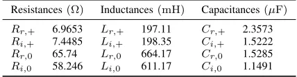
In Table I, the long-line corrected series resistances, series inductances, and shunt capacitances are given for transmission lines Zr andZi shown in Fig. 1. Indicesr andirefer to the

rectifier and inverter systems respectively, while+and0refer to the positive and zero sequence values respectively.

The link used a marginal current control method with DC-side current, DC-side voltage, and extinction angle error loops at both the inverter and the rectifier, as shown in Fig. 2. The link used VDCOLs at both the rectifier and inverter to reduce ordered DC-side current at their corresponding converter station when measured DC-side voltage reduced below a threshold.

The VDCOL characteristic used ordered DC-side current ramp up and ramp down rate limiters in conjunction with

TABLE I

AC-SIDETRANSMISSIONLINEPOSITIVE ANDZEROSEQUENCE IMPEDANCES ATPOWERFREQUENCY

Resistances(Ω) Inductances(mH) Capacitances(µF)

Rr,+ 6.9653 Lr,+ 197.11 Cr,+ 2.3573

Ri,+ 7.4485 Li,+ 198.35 Ci,+ 1.5222

Rr,0 65.74 Lr,0 664.17 Cr,0 1.5285

Ri,0 58.246 Li,0 611.17 Ci,0 1.1491

a steady-state piecewise-linear voltage-current characteristic. Both the inverter and rectifiers used the same VDCOL design; the DC-side current margin was used to separate the VDCOL characteristics between the rectifier and inverter to ensure a single steady state operating point.

The optimisation problems we used to compare the solver methods are controller tuning problems of a LCC-HVDC link model similar to those in [3]. The controller parameters to be optimised were: PI controller proportional gain and integral time constant; and VDCOL upper DC-side voltage breakpoint and current ramp up and down rate limits. These variables were tuned with respect to external disturbances and a power set-point change. The disturbances included: inverter AC-side voltage magnitude and phase deviations and recoveries; and a short circuit fault at the inverter AC-side busbar. We studied two Problems: one where only PI controller gains were tuned, and another where PI controller gains and VDCOL parameters were tuned simultaneously. The Problems’ objective was to control a measured DC-side power towards an ordered value.

min over 1 cycle

γ

α*

αLB αUB

1

τint s

Kp +

1 0.02s + 1

Ramp Rate Limiter (I'up , I'dn)

VDC

0.65 1 0.02s + 1

9.4838

min selector 3.8637

|u |

0.1 1.1

min selector 1.10

0.35 0.4 Vh

d

n _n

d

1 0.02s + 1 PDC*

ΔIDC

IDC _0.0021_s_{+ 1}

VDC*

ΔVDC γ*

Fig. 2. Control diagram of converter controllers. Measured extinction angle γwas the minimum of the extinction angles measured from that converter station’s thyristor bridges. Ordered delay angleα∗_{was sent to both thyristor bridges of that converter station.}_P

DC∗= 1 pu,γ∗= 18◦, andVDC∗= 1 pu

nominally. At the rectifier;∆IDC = 0 pu,∆VDC = 2 pu, andαUB= 90◦andαLB = 5◦. At the inverter;∆IDC = 0.1 pu,∆VDC = 0 pu, and αUB_{= 180}◦_and_αLB_{= 90}◦_._V

h,Iup0 ,Idn0 ,Kp, andτintwere optimisation problem variables; each converter station had uniqueKpandτint, butVh, I0

[image:3.612.330.544.89.145.2]

(4)

III. DESCRIPTION OFOPTIMISATIONPROBLEMS

We focus on the motivating problem of selecting controller parameters for a back-to-back LCC-HVDC scheme, which we consider mathematically as a m-variable box constrained optimisation problem in the form of (1), where x ∈ Rm,

f :_Rm_7→

R.f is assumed to be non-smooth and non-linear.

minf(x), s.t. XLB≤x≤XUB (1) We define the error signal e in (2) as the difference between ordered and measured DC-side powers PDC∗

and PDC, respectively. Note that the error e was in

general a function of time t, and parametrised by controller parameters x, a particular combination of disturbances and set-point changes d, and operational scenario s. Measured DC-side power was simply calculated from the measured DC-side voltage and current viaPDC=VDC·IDC.

e(t;x, d, s) =PDC∗(t;x, d, s)−PDC(t;x, d, s) (2)

We define a function ISEd as being the approximate ISE of the error functione, calculated using the trapezoidal rule with fixed interval lengths. We simply summed the approximate ISEs of all operational scenarios s in the set of operational scenariosS to give the overall objective functionf in (3).

f(x;d) =X s∈S

d

ISE [e(t;x, d, s)] (3)

In our studies, S was a set with two members: one for an inverter AC system with ESCR = 1.9 and another with ESCR = 3.0. These scenarios were realised by manipulating the inverter remote AC system source resistances and inductance, and the switching in or out of a single inverter AC-side harmonic filter.

A. Problem 1: PI Controller Tuning

With reference to Figs. 1 and 2, in Problem 1 we tuned only the four PI controller parameters subjected to the following combination of power set-point changes and disturbances at simulation time step t as follows:

1) t= 0.1 s: δi =−7.5 deg;

2) t= 0.6 s: δi = 0.0 deg;

3) t= 1.1 s: Vi= 0.93 pu;

4) t= 1.6 s: Vi= 1.0 pu;

5) t= 2.1 s: PDC∗= 0.5 pu;

6) t= 2.6 s: PDC∗= 1.0 pu;

Problem 1 can be considered as a specific realisation of (1) with XLB ₌ _[0_.₀₁_,₀_.₀₁_,₀_.₀₁_,₀_._01]_, _XUB ₌ [1.0,1.0,1.0,1.0], andx= [Kr,p, τr,int, Ki,p, τi,int].

B. Problem 2: PI Controller and VDCOL Tuning

In Problem 2, we tuned the four PI controller parameters as in Problem 1 as well as the three VDCOL parameters for both inverter and rectifier VDCOLs with reference to Figs. 1 and 2, subjected to the following combination of set-point changes and disturbances:

1) t= 0.1 s,θi =−7.5 deg;

2) t= 0.6 s,θi= 0.0 deg;

3) t= 1.1 s,Vi= 0.93 pu;

4) t= 1.6 s,Vi= 1.0 pu;

5) t= 2.1 s,PDC∗= 0.5 pu;

6) t= 2.6 s,PDC∗= 1.0 pu;

7) t= 4.0 s,CB1closed;

8) t= 4.01667 s,PDC∗= 0.0 pu;

9) t= 4.05 s,CB1opened;

10) t= 4.05667 s,PDC∗= 1.0 pu;

Problem 2 can be considered as a particular realisation of (1) with x = Kr,p, τr,int, Ki,p, τi,int, Vh, Iup0 , Idn0

,

XLB= [0.01,0.01,0.01,0.01,0.52,0.667,0.667]andXUB= [1.0,1.0,1.0,1.0,0.95,66.7,66.7].

Note that this approach tuned both converters’ PI controller and VDCOL parameters simultaneously. This is in contrast with the approach taken in [3] which tuned PI parameters first, fixed the PI parameters at their optimal values, and then tuned the VDCOL parameters.

After the fault application at t = 4.0 s, note that the link power transfer was reduced to zero after one cycle. Once the fault was cleared, the link ordered power transfer was then returned back to nominal after waiting one cycle after fault clearance. The purpose of this transient ordered power reduction was to reduce the contribution to the objective function value due to a large unavoidable tracking error caused by the fault application. During the fault, no DC-side power could be transferred as the fault caused zero AC-side voltage magnitude. Hence the fault-on period would contribute a large and almost static integral error to the objective function value, which could not be reduced by the choice of optimisation variables.

In our work, we do not remove the inverter AC-side busbar from service on clearance of the fault—this is a simplification from a realistic power system, where a busbar fault would be cleared by switching out the busbar.

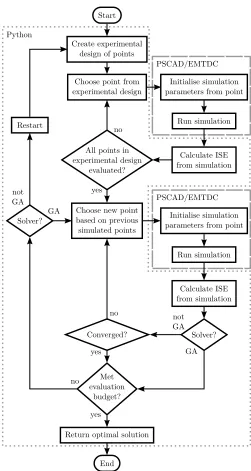
IV. DESCRIPTIONS OFTESTEDSOLVERMETHODS

We studied four solver strategies, all of which were initialised using an experimental design. All solver implementations were set to terminate on a given maximum evaluation budget. Note that all solvers apart from Solver GA allowed restarting during the solution process; this allowed extra experimental designs to be undertaken when objective function values appeared to be converging. Restarting allowed further exploration of the problem space within the defined evaluation budget.

A. Initial Experimental Design

(5)

B. Solver MARS

This solver used a surrogate model to approximate the expensive objective function. An initial experimental design provided a set of initial points and corresponding objective function values, which were then used to fit the surrogate model. A sampling strategy then used the fitted surrogate model to find a small number of new, promising points to then be evaluated through the expensive objective function. If the solver detected solution convergence but still had remaining evaluations available, it would restart by performing a new 22 point experimental design within the remaining evaluation budget. This allowed efficient use of expensive objective function evaluations since the surrogate was cheap to evaluate, with the result of the expensive evaluation being used to update the surrogate model. This process continued until the evaluation budget was completely used.

The sampling strategy we used to find promising candidate points from the fitted surrogate model was dynamic coordinate search using response surface models (DYCORS), specifically DYCORS-LMSRBF from [7]. Multivariate adaptive regression splines (MARS) [8] formed the surrogate model.

C. Solver GPR

This solver’s architecture was almost identical to that of Solver MARS, but with one difference. We used a Gaussian process regression (GPR) [9] surrogate model for Solver GPR as opposed to the MARS surrogate model in Solver MARS.

D. Solver NM

This solver used an initial experimental design to sample the expensive objective function in the same manner as Solvers MARS and GPR. The m+ 1 points with the best objective function values for a m-variable problem were then used to construct the m+ 1 initial vertices used by a Nelder-Mead solution algorithm [4], which is an unconstrained method. To implement support for box constraints, we used a variable transformation method shown in (4) and (5) to transform the i-th external problem variable xi bounded by

upper boundX_iUBand lower boundX_iLB, to and from internal variableyi used within the Nelder-Mead solver algorithm.

yi= arcsin

2· xi−X LB i

XUB i −XiLB

−1

(4)

xi =

XUB i −XiLB

2 (sin (yi) + 1) +X LB

i (5)

E. Solver GA

This solver used a real-valued genetic algorithm, where: selection was via a tournament; mutations were normally distributed perturbations; crossovers were implemented using a linear combination of parents at a uniformly randomly generated cutting point; and there was a single elite population member.

no yes

yes no

Initialise simulation parameters from point

Run simulation

Calculate ISE from simulation All points in

experimental design evaluated?

Converged? Choose new point based on previous simulated points Choose point from experimental design Create experimental design of points

End Start

PSCAD/EMTDC Python

Solver?

Met evaluation

budget? Restart

yes

not GA

GA Solver? GA

not GA

no

Return optimal solution

Initialise simulation parameters from point

Run simulation

[image:5.612.311.562.44.515.2]

Calculate ISE from simulation PSCAD/EMTDC

Fig. 3. Indicative flowchart of the simulation-based optimisation procedure; note the delineation between the Python interpreter process and the PSCAD/EMTDC process.

V. IMPLEMENTATIONDETAILS

(6)

budget, and to avoid repeated function evaluations of the elite population member. Solver NM was implemented using modified code fromscipy[11], where the modifications were to incorporate the variable transformations of (4) and (5). The termination condition of the Nelder-Mead algorithm in Solver NM was set to an absolute objective function value tolerance of 0.01. All four solvers’ parameters were otherwise set to default values in all cases.

VI. ASSESSMENTSTRATEGY

The stochastic nature of the solvers required statistical methods to competently compare the relative performance of the solvers. We used a pairwise comparison approach: since we studied four solvers, there were six possible comparisons to be made between pairs of solvers. We used a nonparametric bootstrap method to compare the mean optimal solution objective function values of the four solvers to detect if their was a statistical difference between a pair of solver means.

We performed 30 independent optimisation runs of each solver on both Problems. For each solver, we therefore had: two samples (one each per Problem) where each sample contained 30 observations. Each observation was the objective function value of the returned optimal solution. We set a maximum evaluation budget of 200 evaluations of the simulation model for each solver, thus the observed objective function value was the lowest found within the 200 evaluations. We then used these samples to determine if there was a statistical difference between the sample means of two solvers for the same Problem.

The solver computational time was negligible for all solvers and so their contribution to the overall optimisation computational time was small compared to the objective function evaluations. Solvers that performed significantly better within 200 objective function evaluations were therefore assumed to be significantly better options with respect to overall solution time.

The aim of the nonparametric bootstrap method was to infer the population difference δ between two solvers’ expected valuesµ of the objective function at the optimal solutions.

We assume that the optimal solution objective function value of a particular solver for a Problem is a random variableW, with an unknown distributionF, and an excepted value E[W] = µ1. Similarly, another solver applied to the

same Problem returns an optimal solution objective function value which is another random variable V, with its own unknown distribution G, and an excepted valueE[V] =µ2.

Our approach was to make inferences about the population parameter δ, where δ = µ1 − µ2. As µ1, µ2, and

therefore δ were population parameters and thus unknown, we used sampling with subsequent bootstrap re-sampling to estimate confidence intervals for δ for each of the six solver comparisons.

We draw a sampleWof optimal solution objective function values for one solver by sampling from F. The sample W is a set, where W = {wk:k∈ N }, N = {1,2, ..., n},

and n = 30. We then draw a sample V of optimal solution

objective function values for the other solver by sampling fromG. The sampleVis also a set, whereV={vk:k∈ N }.

We then produce a set W∗ _{of a very large number} _B of re-samples W∗

b of W by uniform re-sampling with

replacement; whereB= 105_,_W∗

b is theb-th re-sample ofW,

andW∗

b ={W1∗,W2∗, ...,WB∗}. We generate a similar setV∗

of re-samplesV∗

b from V. Note that each Wb∗ andVb∗ are of

cardinalityn,i.e.the cardinality of the samples W andV. We then calculate a statistic set Q∗ _{from the sets of} re-samplesW∗ _and_V∗ _{as in (6).}

Q∗= ₁

n

X

W_b∗−XV_b∗−

1

n

X

W −XV:b∈ {1,2, ..., B}

(6)

We define the quantile function Jˆ(p), which returns the quantile for a specified probability p using a linear interpolation method—specificallyDefinition 7 from [12]—on the empirical cumulative distribution of Q∗_. _Jˆ₍_p₎ _{may then} be used to estimate a confidence interval forδ, the difference in the expected values of the two solvers. For a confidence level of 95%, the estimated lowerδLB and upperδU B bounds

of δare given by (7) and (8) respectively.

δLB = 1

n

X

W −XV−Jˆ(0.975) (7)

δU B = 1

n

X

W −XV−Jˆ(0.025) (8)

VII. RESULTS ANDDISCUSSION

Figs. 4, 5, and 6 show selected system variables over time for both Problems when ESCR = 3.0 for the best found optimal solution in all 30 runs per solver. Trace colour darkens where the grey traces overlap. Traces appear thick due to ripple in both the DC-side current and DC-side voltage. Disturbances in the variables over time coincide with the applied external disturbances and ordered power set-point changes listed in Sections III-A and III-B.

[image:6.612.357.556.350.416.2]

We include Figs. 4, 5, and 6 to show that all four solvers are capable of solving the box constrained Problems effectively, with the best solutions giving broadly qualitatively consistent time domain responses between solvers. Note that the best time domain responses per solver for ESCR = 1.9 are similarly consistent.

(7)

0.0 0.8 1.6 2.4 3.2 4.0

−0.2 0.0 0.2 0.4 0.6 0.8 1.0

Measured

DC-Side

P

o

w

er

(pu)

Problem 1: PI Controller Tuning

NM MARS GPR GA

0.0 1.2 2.4 3.6 4.8 6.0

Simulation Time (s)

−0.2 0.0 0.2 0.4 0.6 0.8 1.0

Measured

DC-Side

P

o

w

er

(pu)

Problem 2: PI Controller and VDCOL Tuning

NM MARS GPR GA 2.5 2.7 2.9 3.1

0.4 0.6 0.8 1.0 1.2

3.98 4.06 4.14 4.22 0.0

[image:7.612.318.555.55.337.2]

0.5 1.0

Fig. 4. DC-side power over time.

0.0 0.8 1.6 2.4 3.2 4.0

−0.2 0.0 0.2 0.4 0.6 0.8 1.0

Measured

DC-Side

V

oltage

(pu)

NM MARS GPR GA

0.0 1.2 2.4 3.6 4.8 6.0

Simulation Time (s)

−0.2 0.0 0.2 0.4 0.6 0.8 1.0

Measured

DC-Side

V

oltage

(pu)

NM MARS GPR GA 2.5 2.7 2.9 3.1

0.4 0.6 0.8 1.0 1.2

3.98 4.06 4.14 4.22 0.0

[image:7.612.56.293.58.340.2]

0.5 1.0

Fig. 5. DC-side voltage over time.

0.0 0.8 1.6 2.4 3.2 4.0

−0.2 0.0 0.2 0.4 0.6 0.8 1.0 1.2

Measured

A

C-Side

V

oltage

(pu)

NM MARS GPR GA

0.0 1.2 2.4 3.6 4.8 6.0

Simulation Time (s)

−0.2 0.0 0.2 0.4 0.6 0.8 1.0 1.2

Measured

A

C-Side

V

oltage

(pu)

NM MARS GPR GA 2.5 2.7 2.9 3.1

0.4 0.6 0.8 1.0 1.2

3.98 4.06 4.14 4.22 0.0

[image:7.612.59.293.68.600.2]

0.5 1.0

Fig. 6. AC-side voltage magnitude at the inverter AC-side busbar over time.

For Problem 1, both Solvers GPR and MARS perform better than Solver GA. However, Solvers GPR and MARS are similar, and Solver NM is similar to all three other Solvers. In Problem 2, only Solvers GA and GPR are similar; all other Solver comparisons show significant differences between means. Solver MARS outperforms all other Solvers, while Solvers GA and GPR outperform Solver NM.

Qualitatively, the solvers’ relative performances are very close for Problem 1 where only the PI controller parameters are tuned. However, relative performances are much more disparate for the more difficult Problem 2 where PI and VDCOL parameters are tuned together.

At no point did either Solvers NM or GA perform significantly better than Solvers MARS or GPR for either Problem. Our results suggest that for the Problems we studied, practitioners should be confident in using Solvers MARS or GPR in place of the benchmark methods of Solvers GA and NM.

[image:7.612.56.295.360.661.2]

(8)

GA

GPR MARSGA MARSGPR NMGA GPRNM MARSNM

−0.02 0.00 0.02 0.04

Statistical

Difference

of

Solv

er

Mean

Optimal

Solutions

GA

GPR MARSGA MARSGPR NMGA GPRNM MARSNM Comparison

−0.25 0.00 0.25 0.50 0.75 1.00

Statistical

Difference

of

Solv

er

Mean

Optimal

Solutions

Problem 2: PI Controller and VDCOL Tuning GPR

MARS

−0.002

[image:8.612.319.556.54.336.2]

−0.001 0.000

Fig. 7. Comparisons of difference in mean optimal solutions between pairs of solvers. Points are observed differences in sample means; intervals are the estimates of the difference in expected values at the 95% confidence level.

VIII. CONCLUSIONS

Tuning of LCC-HVDC link controller parameters is important to ensure adequate operation of the link during normal set-point changes and disturbances. Surrogate model methods are used in this paper to optimize these controller parameters as box constrained, simulation-based optimisation problems. Using the integral-square-error between ordered and measured HVDC link power transfer, the firing angle PI controller and VDCOL parameters are optimized using time domain simulations, considering: power set-point changes, inverter AC-side voltage disturbances, and an inverter AC-side short circuit fault. The MARS and GPR surrogate model methods provided similar or significantly better optimal solutions when compared to the mature solver methods that we used as benchmarks. This paper demonstrates the increasing competitiveness of simulation-based optimisation as a tool for efficiently solving parameter selection problems in power system engineering, particularly where non-linear behaviour such as large power system transients must be considered.

REFERENCES

[1] A. M. Gole, S. Filizadeh, R. W. Menzies, and P. L. Wilson, “Electromagnetic transients simulation as an objective function evaluator for optimization of power system performance,” in International

Conference on Power Systems Transients, Sep. 2003, pp. 1–6.

0 25 50 75 100 125 150 175 200

0.0 0.2 0.4 0.6 0.8 1.0 1.2

Ob

jectiv

e

F

unction

V

alue

NM MARS GPR GA

0 25 50 75 100 125 150 175 200

Objective Function Evaluation 0.0

0.8 1.6 2.4 3.2 4.0 4.8

Ob

jectiv

e

F

unction

V

alue

NM MARS GPR GA

180 190 200

0.025 0.045 0.065 0.085

180 190 200

0.3 0.6 0.9 1.2 1.5

Fig. 8. Convergence plots per solver. Trace colour darkens where the grey traces overlap. Lines indicate observed sample mean while shaded bands show estimated sample mean 95% confidence intervals also calculated via nonparametric bootstrapping, both over all 30 runs.

[2] ——, “Optimization-enabled electromagnetic transient simulation,”

IEEE Transactions on Power Delivery, vol. 20, no. 1, pp. 512–518,

Jan. 2005.

[3] S. Filizadeh, A. M. Gole, D. A. Woodford, and G. D. Irwin, “An optimization-enabled electromagnetic transient simulation-based methodology for HVDC controller design,”IEEE Transactions on Power

Delivery, vol. 22, no. 4, pp. 2559–2566, Oct. 2007.

[4] J. A. Nelder and R. Mead, “A simplex method for function minimization,”The Computer Journal, vol. 7, no. 4, pp. 308–313, Jan. 1965.

[5] A. Y. Goharrizi, R. Singh, A. M. Gole, S. Filizadeh, J. C. Muller, and R. P. Jayasinghe, “A parallel multimodal optimization algorithm for simulation-based design of power systems,” IEEE Transactions on

Power Delivery, vol. 30, no. 5, pp. 2128–2137, Oct. 2015.

[6] K. Q. Ye, W. Li, and A. Sudjianto, “Algorithmic construction of optimal symmetric latin hypercube designs,”Journal of Statistical Planning and

Inference, vol. 90, no. 1, pp. 145–159, Sep. 2000.

[7] R. G. Regis and C. A. Shoemaker, “Combining radial basis function surrogates and dynamic coordinate search in high-dimensional expensive black-box optimization,”Engineering Optimization, vol. 45, no. 5, pp. 529–555, Jun. 2013.

[8] J. H. Friedman, “Multivariate adaptive regression splines,”Annals of

Statistics, vol. 19, no. 1, pp. 1–67, Mar. 1991.

[9] C. E. Rasmussen and C. K. I. Williams,Gaussian Processes for Machine

Learning. MIT Press, 2005, alg. 2.1, p. 19.

[10] D. Eriksson, D. Bindel, and C. Shoemaker. (2015) Surrogate optimization toolbox (pySOT). Version 0.1.36. [Online]. Available: www.github.com/dme65/pySOT

[11] E. Jones, T. Oliphant, P. Peterson, and others. (2001) SciPy: Open source scientific tools for Python. Version 1.1.0. [Online]. Available: www.scipy.org

[12] R. J. Hyndman and Y. Fan, “Sample quantiles in statistical packages,”

[image:8.612.59.293.58.353.2]