City, University of London Institutional Repository
Citation: Karabag, C., Verhoeven, J. ORCID: 0000-0002-0738-8517, Miller, N. and
Reyes-Aldasoro, C. C. ORCID: 0000-0002-9466-2018 (2019). Texture Segmentation: An
Objective Comparison between Traditional and Deep-Learning Methodologies. Preprints,
doi: 10.20944/preprints201908.0001.v1
This is the draft version of the paper.
This version of the publication may differ from the final published
version.
Permanent repository link: http://openaccess.city.ac.uk/id/eprint/22870/
Link to published version: 10.20944/preprints201908.0001.v1
Copyright and reuse: City Research Online aims to make research
outputs of City, University of London available to a wider audience.
Copyright and Moral Rights remain with the author(s) and/or copyright
holders. URLs from City Research Online may be freely distributed and
linked to.
City Research Online:
http://openaccess.city.ac.uk/
[email protected]
Article
Texture segmentation: an objective comparison
between traditional and deep-learning methodologies
Cefa Karaba ˘g1, Jo Verhoeven2,3, Naomi Rachel Miller2and Constantino Carlos Reyes-Aldasoro1,?
1 Department of Electrical and Electronic Engineering, Research Centre for Biomedical Engineering, School of
Mathematics, Computer Science and Engineering, City, University of London, London EC1V 0HB, UK
2 School of Health Sciences, Division of Language & Communication Science, Phonetics Laboratory, City,
University of London, UK; [email protected], [email protected]
3 Department of Linguistics CLIPS, University of Antwerp, Antwerp, Belgium; [email protected]
1 2 3 4 5 6 7 8
* Correspondence:[email protected](CCRA)
Abstract: This paper comparesaseries of traditional anddeep learningmethodologies for the segmentationoftextures.Sixwell-knowntexturecompositesfirstpublishedbyRandenandHusøy wereusedtocomparetraditionalsegmentationtechniques(co-occurrence, filtering,localbinary patterns,watershed,multiresolutionsub-bandfiltering)againstadeep-learningapproachbasedon theU-Netarchitecture. Forthelatter,theeffectsofdepthofthenetwork,numberofepochsand differentoptimisationalgorithmswereinvestigated.Overall,thebestresultswereprovidedbythe deep-learningapproach.However,thebestresultsweredistributedwithintheparameters,andmany configurationsprovidedresultswellbelowthetraditionaltechniques.
Keywords:Texture;Segmentation;DeepLearning
9
1. Introduction
10
Texture, and more specifically textural characteristics in images, has been widely studied in the
11
past decades as texture is one of the most important features present in images and can be used for
12
feature extraction [1–8] and classification and segmentation [9–14]. The areas of study where texture
13
is present range from crystallographic texture [15], stratigraphy [16,17], food science of potatoes [18]
14
or apples [19], patterned fabrics [20] to natural stone industry [21]. In medical imaging, there is a
15
large volume of research which exploits the use of texture for different purposes like segmentation of
16
classification in most acquisition modalities like magnetic resonance imaging (MRI) [22–26], ultrasound
17
[27,28], computed tomography (CT) [29–31], microscopy [32,33] and histology [34]. There are numerous
18
approaches to texture: Haralick’s co-occurrence matrix [4,5] on the spatial domain, Gabor filters [35–37]
19
and ordered pyramids [8] on the spectral domain, wavelets [38,39] or Markov random fields [3,40].
20
In recent years, advances in artificial intelligence have been revolutionised image processing tasks.
21
Several deep learning approaches [41–43] have achieved outstanding results in difficult tasks such
22
as those of the ImageNet Large Scale Visual Recognition Challenge (ILSVRC) [44]. Convolutional
23
Neural Networks (CNNs) are well suited to analyse textures as their repetitive patterns can be learned
24
and identified by filter banks [45]. The U-Net architecture proposed by Ronneberger [46] has become
25
a very widely used tool for segmentation and analysis reaching thousands of citations in few years
26
since it was published. U-Nets have been used widely, for instance, road extraction [47], singing voice
27
separation [48], automatic brain tumour detection and segmentation [49] and cell counting, detection,
28
and morphometry [50]. The success of these deep learning approaches in very different areas invite for
29
its application on texture analysis.
30
In this work, a U-Net architecture for the segmentation of textures is implemented and objectively
31
compared against several popular traditional segmentation strategies. To perform an objective
32
comparison, six well-known texture composites from the Brodatz [51] album, first published by Randen
33
and Husøy [52], are segmented with U-Nets of different configurations and parameters and the results
34
compared against previously published results. The effects of the configuration of the networks, namely,
35
number of epochs, depth of the network in the number of layers, and type of optimisation algorithm
36
are assessed. All the programming was performed in MatlabR (The MathworksTM, Natick, USA) and
37
the code is freely available through GitHub (https://github.com/reyesaldasoro/Texture-Segmentation).
38
2. Materials and Methods
39
2.1. Texture composite images
40
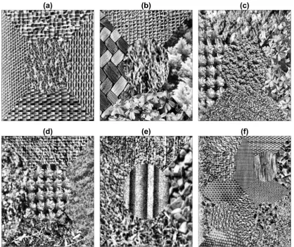
Six composite texture images were segmented in this work (Fig.1). The first five composites are
41
images of 256
×
256 pixels and consist of five different textures whilst the last one is 512×
512 pixels42
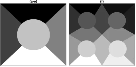
and is formed with 16 different textures. The masks with which these were formed are shown in Fig.2.
43
It should be highlighted that these textures have been histogram equalised prior to the arrangement
44
and thus they cannot be distinguished by the general intensity of each region. Furthermore, whilst
45
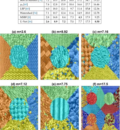
some textures are easy to distinguish, there are some that are quite challenging, for instance, the
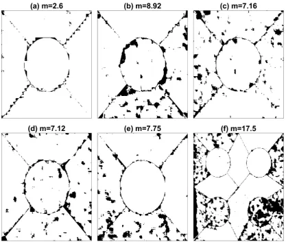
46
difference between the central and bottom regions in Fig.1(c) or the top left corners of Fig.1(d,e).
[image:3.595.87.506.334.685.2]47
Figure 2.(a) Mask corresponding to texture arrangements of Figs.1(a-e). (b) Mask corresponding to
texture arrangements of Fig.1(f).
2.2. Training data
48
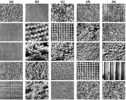
The training data in [52] is provided separately and is shown in Fig.3for the first five composites
49
and in Fig.4for the last case. For the purpose of training the U-Nets, the training images were
50
tessellated into sub-regions of 32
×
32 pixels each.51
Pairs of textures and labels were constructed simultaneously in the following way: two training
52
images were selected. Sub-regions of each image were selected and for every pair of the sub-regions,
53
half of each was selected and placed together so that a new 32
×
32 patch with both textures was54
created with a corresponding 32
×
32 patch with the classes. The patches were created with diagonal,55
vertical and horizontal pairs. The training images were traversed horizontally and vertically without
56
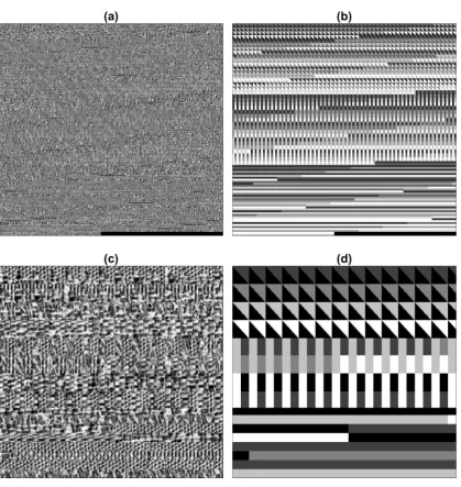
overlap creating numerous training pairs. A montage of the texture pairs and labels corresponding to
57
Fig.1(a) is illustrated in Fig.5. All pairs between classes were considered i.e. 1
−
2, 1−
3, 1−
4, 1−
58
5, 2
−
1, 2−
3, . . . , 5−
3, 5−
4. In total, 2, 940 patches were created for the five composites with five59
textures and 35, 280 were created for the composite with sixteen textures.
Figure 5.Montages of the texture pairs created to train the deep learning networks. Training images
shown in Figs.3,4were tessellated and arranged in diagonal, vertical and horizontal pairs. (a) Texture
pairs. (b) Labels. (c) Detail of the texture pairs. (d) Detail of the labels.
2.3. Texture segmentation algorithms
61
For this paper, we compared the results of the following texture segmentation algorithms:
62
co-occurrence matrices [5], filtering [52], Local Binary Patterns (LBP) [53], watershed [54] and
63
multiresolution sub-band filtering (MSBF) [8] against a U-Net architecture [46]. As the traditional
64
algorithms have been thoroughly described in the literature, this section will only describe the
65
configuration of the U-Net. For a review of traditional texture techniques, the reader is referred
66
to any of the following reviews [55–57].
67
The basic U-Net architecture was formed with the following layers:Input, Convolutional, ReLu,
68
Max Pooling, Transposed Convolutional, Convolutional, SoftmaxandPixel Classification. Two levels of
69
depth were investigated by repeating the downsampling and upsampling blocks in the following
70
configurations:
71
15 layers:
72
Input,
Convolutional, ReLu, Max Pooling,
74
Convolutional, ReLu, Max Pooling,
75
Convolutional, ReLu,
76
Transposed Convolutional, Convolutional,
77
Transposed Convolutional, Convolutional,
78
Softmax,
79
Pixel Classification
80 81
20 layers:
82
Input,
83
Convolutional, ReLu, Max Pooling,
84
Convolutional, ReLu, Max Pooling,
85
Convolutional, ReLu, Max Pooling,
86
Convolutional, ReLu,
87
Transposed Convolutional, Convolutional,
88
Transposed Convolutional, Convolutional,
89
Transposed Convolutional, Convolutional,
90
Softmax,
91
Pixel Classification.
92 93
The image input layer was configured for the 32
×
32 patches. The convolutional layers consisted94
of 64 filters of size 3 and padding of 1. The pooling size was 2 with stride of 2. The transposed
95
convolutional had a filter size of 4, stride of 2 and cropping of 1. The number of epochs evaluated
96
were 10, 20, 50, 100. The following optimisation algorithms were analysed: stochastic gradient descent
97
(sgdm), Adam (Adam) [58] and Root Mean Square Propagation (RMSprop). One last investigation
98
was performed by training the 20 layer network two separate times to investigate the variability of the
99
process.
100
3. Results
101
For each image, the networks were trained with the 3 different optimisation algorithms, 3 layer
102
configurations and 4 epoch numbers, for a total of 36 different combinations. Thus for the 6 composites
103
images there were 216 results. The misclassification of each segmentation was measured against the
104
ground truth as the percentage of pixels classified incorrectly. These results are summarised in table1.
105
The best results for each image were selected and compared against traditional methodologies
106
and are shown in table2. The results are illustrated graphically in two ways. Fig.6shows segmented
107
the classes overlaid as different colours over the original textured images. Fig.7shows correctly
108
segmented pixels in white and the misclassified pixels in black.
Table 1. Comparative misclassification (%) results of the different U-Net configurations. (Bold and underline denotes the best result for each image).
Method Figures
Layers Optimisation Algorithm Epochs a b c d e f
15 sgdm 10 6.8 21.5 40.8 31.2 27.2 20.9
20 sgdm 10 33.0 59.0 74.3 79.1 77.3 41.9
20 sgdm 10 71.9 62.9 74.3 78.8 72.1 39.0
15 Adam 10 3.2 10.4 7.9 7.1 17.8 19.3
20 Adam 10 7.4 15.5 46.5 25.0 45.1 94.2
20 Adam 10 6.4 15.5 36.0 21.1 26.7 32.9
15 RMSprop 10 5.1 8.9 14.0 18.3 12.1 17.6
20 RMSprop 10 5.3 42.4 45.3 59.9 56.2 27.7
20 RMSprop 10 20.2 37.4 47.0 43.7 44.2 26.1
15 sgdm 20 3.8 23.1 17.5 15.9 14.1 19.8
20 sgdm 20 27.3 60.5 74.8 69.3 73.9 27.4
20 sgdm 20 23.8 51.0 63.6 66.8 56.5 26.7
15 Adam 20 3.7 11.6 7.5 7.4 9.5 71.7
20 Adam 20 6.1 13.3 28.7 18.5 40.8 32.2
20 Adam 20 5.6 17.9 27.4 22.5 39.3 94.0
15 RMSprop 20 3.8 11.7 14.5 19.2 11.7 17.9
20 RMSprop 20 6.1 42.2 54.7 47.5 42.6 22.3
20 RMSprop 20 19.1 30.3 44.7 51.7 37.1 26.9
15 sgdm 50 3.2 15.3 9.2 7.7 13.8 19.6
20 sgdm 50 18.2 32.2 60.3 42.8 30.2 28.9
20 sgdm 50 9.4 55.2 56.0 16.0 32.4 32.4
15 Adam 50 3.4 10.4 9.8 9.9 39.1 22.6
20 Adam 50 8.3 80.3 19.8 82.3 79.6 34.8
20 Adam 50 7.2 9.6 41.4 10.0 27.6 23.6
15 RMSprop 50 3.4 18.7 10.0 8.3 11.2 17.5
20 RMSprop 50 5.6 33.2 25.7 34.8 34.4 22.4
20 RMSprop 50 5.4 22.8 45.3 20.0 34.7 29.2
15 sgdm 100 3.9 10.6 7.9 7.7 7.7 21.4
20 sgdm 100 9.6 22.1 39.4 39.7 30.3 23.8
20 sgdm 100 13.7 17.1 52.8 26.3 37.1 30.5
15 Adam 100 2.7 16.6 80.3 7.2 18.2 21.9
20 Adam 100 2.6 38.9 79.9 80.1 31.1 25.7
20 Adam 100 3.4 80.0 79.7 80.9 80.3 28.6
15 RMSprop 100 4.8 11.2 7.2 8.1 9.5 18.1
20 RMSprop 100 7.1 66.0 46.0 28.6 30.9 24.0
20 RMSprop 100 5.6 29.5 26.9 18.5 29.3 22.9
Max 71.9 80.3 80.3 82.3 80.3 94.1
Mean 10.4 30.7 39.4 33.7 35.6 30.7
Table 2. Comparative misclassification (%) results with co-occurrence [5], best filtering result from
Randen [52],p8and LBP [53], Watershed [54], Multiresolution sub-band filtering (MSBF) [8] and U-Net
[46]. (Bold is the best for each image).
Method Figures
a b c d e f Average
Co-occurrence [5] 9.9 27.0 26.1 51.1 35.7 49.6 33.23
Best in Randen [59] 7.2 18.9 20.6 16.8 17.2 34.7 19.23
p8[60] 7.4 12.8 15.9 18.4 16.6 27.7 16.46
LBP [60] 6.0 18.0 12.1 9.7 11.4 17.0 12.36
Watershed [54] 7.1 10.7 12.4 11.6 14.9 20.0 12.78
MSBF [8] 2.8 14.8 8.4 7.3 4.3 17.9 9.25
U-Net [46] 2.6 8.9 7.2 7.1 7.7 17.5 8.50
[image:10.595.90.503.189.634.2]Figure 7. (a-f) Results of the segmentation with U-Nets for the six texture arrangments. The misclassification (%) is shown in each case. Pixels that are correctly classified appear in white.
4. Discussion
110
The results provided by the U-Net algorithm provided interesting results. First, overall, the
111
segmentation results provided by the U-Net were better than all the traditional algorithms and were
112
the best four of the six images. In some cases, the results were very close to the second best option
113
(a,d,f) and in two cases (e,f) traditional algorithms provided better results. Second, there was a great
114
variability in the results produced by the different configurations. It was surprising that the maximum
115
value of the misclassification in some cases was extremely high, 80% in the cases of 5 textures and
116
94% in the case of 16 textures, those cases are equivalent of selecting a single class for all textures.
117
Third, three of the best results were obtained with 100 epochs, 2 with 10 epochs, and 1 with 50, which
118
is counter-intuitive as it would be expected that longer training times would provide better results.
119
Fourth, three of the best results were provided by RMSprop optimisation, two by Adam and one by
120
sgdm. Finally, and perhaps the most surprising result was that the results provided by the two 20 layer
121
configurations were very different. In a few cases the result were equal (e.g. image c, sgdm, 10 epochs;
122
image b, Adam, 10 epochs) but in others the variation was huge (e.g. image b, Adam, 50 epochs).
123
In terms of texture, it can be highlighted that not all textures are the same, the five textures of
124
image (a) are far easier to distinguish and correctly segment than those of image (b) and image (f). The
125
U-Net was capable of segmenting these textures with accuracy comparable or better than traditional
126
techniques. There are many other configuration parameters that could be varied;learning rate, batch size,
127
variations of the training data, different number of layers, but for the purpose of this work, the results show
128
first, the capability of deep learning architectures for segmentation of textured images and second, in
129
some cases better results that traditional methodologies. However, the configuration of the network
is not trivial and variations of some parameters can provide sub-optimal results. The experiments
131
conducted in this work did not provide conclusive evidence for the selection of any of the parameters
132
evaluated. Furthermore, training of the networks requires considerable resources. The training times
133
for the images with 5 textures took around 5 hours and for the image with 16 textures around 96 hours
134
on a Mac Pro (Late 2013) with a 3.7GHz Quad-Core and 32 GB Memory with Dual AMD FirePro D300
135
graphics processors.
136
Therefore, it can be concluded that U-Net convolutional neural networks can be used for texture
137
segmentation and provide results that are comparable or better than traditional texture algorithms.
138
Furthermore, these results encourage the application of deep learning to other areas, like the texture
139
of voice spectrograms [61]. We can even hypothesise that the images in two dimensions can be
140
decomposed into one-dimensional signals and revisit the analysis of voice signals for the segmentation
141
and classification of phonemes as it was done with early versions of Convolutional Neural Networks
142
[62].
143 144
Acknowledgments:This work was funded by the Leverhulme Trust, Research Project Grant RPG-2017-054.
145
References
146
1. Bigun, J. Multidimensional Orientation Estimation with Applications to Texture Analysis and Optical
147
Flow. IEEE Transactions on Pattern Analysis and Machine Intelligence1991,13, 775–790.
148
2. Bovik, A.C.; Clark, M.; Geisler, W.S. Multichannel Texture Analysis Using Localized Spatial Filters. IEEE
149
Transactions on Pattern Analysis and Machine Intelligence1990,12, 55 – 73.
150
3. Cross, G.R.; Jain, A.K. Markov Random Field Texture Models. IEEE Transactions on Pattern Analysis and
151
Machine Intelligence1983,5, 25–39.
152
4. Haralick, R.M. Statistical and Structural Approaches to Texture. Proceedings of the IEEE1979,67, 786–804.
153
5. Haralick, R.M.; Shanmugam, K.; Dinstein, I. Textural Features for Image Classification. IEEE Transactions
154
on Systems, Man and Cybernetics1973,3, 610–621.
155
6. Tamura, H.; Mori, S.; Yamawaki, T. Texture Features corresponding to Visual Perception. IEEE Transactions
156
on Systems, Man and Cybernetics1978,8, 460–473.
157
7. Tuceryan, M.; Jain, A.K. Texture Analysis. Handbook of Pattern Recognition and Computer Vision, Second
158
ed.; Chen, C.H.; Pau, L.F.; Wang, P.S.P., Eds. World Scientific Publishing, 1998, pp. 207–248.
159
8. Reyes-Aldasoro, C.C.; Bhalerao, A. The Bhattacharyya Space for Feature Selection and Its Application to
160
Texture Segmentation.Pattern Recogn.2006,39, 812–826. doi:10.1016/j.patcog.2005.12.003.
161
9. Bouman, C.; Liu, B. Multiple Resolution Segmentation of Textured Images. IEEE Transactions on Pattern
162
Analysis and Machine Intelligence1991,13, 99–113.
163
10. Jain, A.K.; Farrokhnia, F. Unsupervised texture segmentation using Gabor filters. Pattern Recognition1991,
164
24, 1167– 1186.
165
11. Kadyrov, A.; Talepbour, A.; Petrou, M. Texture Classification with Thousand of Features. British Machine
166
Vision Conference (BMVC); , 2002; pp. 656–665.
167
12. Kervrann, C.; Heitz, F. A Markov Random Field model-based approach to unsupervised texture
168
segmentation using local and global spatial statistics.IEEE Transactions on Image Processing1995,4, 856–862.
169
13. Unser, M. Texture Classification and Segmentation Using Wavelet Frames. IEEE Transactions on Image
170
Processing1995,4, 1549–1560.
171
14. Weszka, J.; Dyer, C.; Rosenfeld, A. A comparative Study of Texture Measures for Terrain Classification.
172
IEEE Transactions Systems, Man and Cybernetics1976,6, 269–285.
173
15. Tai, C.; Baba-Kishi, K. Microtexture studies of PST and PZT Ceramics and PZT Thin Film by Electron
174
Backscatter Diffraction Patterns. Textures and Microstructures2002,35, 71–86.
175
16. Carrillat, A.; Randen, T.; Snneland, L.; Elvebakk, G. Seismic stratigraphic mapping of carbonate mounds
176
using 3D texture attributes. Extended Abstracts, Annual Meeting, European Association of Geoscientists
177
and Engineers; , 2002.
178
17. Randen, T.; Monsen, E.; Abrahamsen, A.; Hansen, J.O.; Schlaf, J.; Snneland, L. Three-dimensional texture
179
attributes for seismic data analysis. Ann. Int. Mtg., Soc. Expl. Geophys., Exp. Abstr.; , 2000.
18. Thybo, A.K.; Martens, M. Analysis of sensory assessors in texture profiling of potatoes by multivariate
181
modelling. Food Quality and Preference2000,11, 283–288. doi:10.1016/S0950-3293(99)00045-2.
182
19. Létal, J.; Jirák, D.; Šuderlová, L.; Hájek, M. MRI ‘texture’ analysis of MR images of apples during ripening
183
and storage. LWT - Food Science and Technology2003,36, 719–727. doi:10.1016/S0023-6438(03)00099-9.
184
20. Lizarraga-Morales, R.A.; Sanchez-Yanez, R.E.; Baeza-Serrato, R. Defect detection on patterned fabrics using
185
texture periodicity and the coordinated clusters representation.Textile Research Journal2017,87, 1869–1882,
186
[https://doi.org/10.1177/0040517516660885]. doi:10.1177/0040517516660885.
187
21. Bianconi, F.; González, E.; Fernández, A.; Saetta, S.A. Automatic classification of granite tiles through colour
188
and texture features.Expert Systems with Applications2012,39, 11212–11218. doi:10.1016/j.eswa.2012.03.052.
189
22. Kovalev, V.A.; Petrou, M.; Bondar, Y.S. Texture Anisotropy in 3D Images. IEEE Transactions on Image
190
Processing1999,8, 346–360.
191
23. Reyes-Aldasoro, C.C.; Bhalerao, A. Volumetric Texture Description and Discriminant Feature Selection for
192
MRI. Proceedings of Information Processing in Medical Imaging; Taylor, C.; Noble, A., Eds.; , 2003; pp.
193
282–293.
194
24. Lerski, R.; Straughan, K.; Schad, L.R.; Boyce, D.; Bluml, S.; Zuna, I. MR Image Texture Analysis - An
195
Approach to tissue Characterization.Magnetic Resonance Imaging1993,11, 873–887.
196
25. Schad, L.R.; Bluml, S.; Zuna, I. MR Tissue Characterization of Intracranial Tumors by means of Texture
197
Analysis.Magnetic Resonance Imaging1993,11, 889–896.
198
26. Reyes Aldasoro, C.C.; Bhalerao, A. Volumetric Texture Segmentation by Discriminant Feature
199
Selection and Multiresolution Classification. IEEE Transactions on Medical Imaging 2007, 26, 1–14.
200
doi:10.1109/TMI.2006.884637.
201
27. Zhan, Y.; Shen, D. Automated Segmentation of 3D US Prostate Images Using Statistical Texture-Based
202
Matching Method. Medical Image Computing and Computer-Assisted Intervention (MICCAI); , 2003; pp.
203
688–696.
204
28. Xie, J.; Jiang, Y.; tat Tsui, H. Segmentation of kidney from ultrasound images based on texture and shape
205
priors.IEEE Transactions on Medical Imaging2005,24, 45–57. doi:10.1109/TMI.2004.837792.
206
29. Hoffman, E.A.; Reinhardt, J.M.; Sonka, M.; Simon, B.A.; Guo, J.; Saba, O.; Chon, D.; Samrah, S.; Shikata,
207
H.; Tschirren, J.; Palagyi, K.; Beck, K.C.; McLennan, G. Characterization of the Interstitial Lung Diseases
208
via Density-Based and Texture-Based Analysis of Computed Tomography Images of Lung Structure and
209
Function. Academic Radiology2003,10, 1104–1118.
210
30. Segovia-Martínez, M.; Petrou, M.; Kovalev, V.A.; Perner, P. Quantifying Level of Brain Atrophy Using
211
Texture Anisotropy in CT Data. Medical Imaging Understanding and Analysis; , 1999; pp. 173–176.
212
31. Ganeshan, B.; Goh, V.; Mandeville, H.C.; Ng, Q.S.; Hoskin, P.J.; Miles, K.A. Non–Small Cell
213
Lung Cancer: Histopathologic Correlates for Texture Parameters at CT. Radiology2013,266, 326–336.
214
doi:10.1148/radiol.12112428.
215
32. Sabino, D.M.U.; da Fontoura Costa, L.; Gil Rizzatti, E.; Antonio Zago, M. A texture approach to leukocyte
216
recognition. Real-Time Imaging2004,10, 205–216. doi:10.1016/j.rti.2004.02.007.
217
33. Wang, X.; He, W.; Metaxas, D.; Mathew, R.; White, E. Cell Segmentation and Tracking using
218
Texture-Adaptive Snakes. 2007 4th IEEE International Symposium on Biomedical Imaging: From Nano to
219
Macro, 2007, p. 101–104. doi:10.1109/ISBI.2007.356798.
220
34. Kather, J.N.; Weis, C.A.; Bianconi, F.; Melchers, S.M.; Schad, L.R.; Gaiser, T.; Marx, A.; Zollner, F. Multi-class
221
texture analysis in colorectal cancer histology | Scientific Reports. Scientific Reports2016,6, 27988.
222
35. Dunn, D.; Higgins, W.; Wakeley, J. Texture segmentation using 2-D Gabor elementary functions. IEEE
223
Transactions on Pattern Analysis and Machine Intelligence1994,16, 130–149.
224
36. Bigun, J.; du Buf, J.M.H. N-Folded Symmetries by Complex Moments in Gabor Space and Their Application
225
to Unsupervised Texture Segmentation.IEEE Transaction on Pattern Analysis and Machine Intelligence1994,
226
16, 80–87.
227
37. Bianconi, F.; Fernández, A. Evaluation of the effects of Gabor filter parameters on texture classification.
228
Pattern Recognition2007,40, 3325 – 3335. doi:https://doi.org/10.1016/j.patcog.2007.04.023.
229
38. Rajpoot, N.M. Texture Classification Using Discriminant Wavelet Packet Subbands. Proceedings 45th IEEE
230
Midwest Symposium on Circuits and Systems (MWSCAS 2002); , 2002.
231
39. Chang, T.; Kuo, C.C.J. Texture Analysis and Classification with Tree-Structured Wavelet Transform. IEEE
232
Transactions on Image Processing1993,2, 429–441.
40. Chellapa, R.; Jain, A.Markov Random Fields; Academic Press: Boston, 1993.
234
41. Krizhevsky, A.; Sutskever, I.; Hinton, G.E. ImageNet Classification with Deep Convolutional Neural
235
Networks. Proceedings of the 25th International Conference on Neural Information Processing Systems
-236
Volume 1. Curran Associates Inc., 2012, NIPS’12, p. 1097–1105. event-place: Lake Tahoe, Nevada.
237
42. Zeiler, M.D.; Fergus, R. Visualizing and Understanding Convolutional Networks. Computer Vision –
238
ECCV 2014; Fleet, D.; Pajdla, T.; Schiele, B.; Tuytelaars, T., Eds. Springer International Publishing, 2014,
239
Lecture Notes in Computer Science, p. 818–833.
240
43. Simonyan, K.; Zisserman, A. Very Deep Convolutional Networks for Large-Scale Image Recognition.
241
arXiv:1409.1556 [cs]2014. arXiv: 1409.1556.
242
44. Russakovsky, O.; Deng, J.; Su, H.; Krause, J.; Satheesh, S.; Ma, S.; Huang, Z.; Karpathy, A.; Khosla, A.;
243
Bernstein, M.; Berg, A.C.; Fei-Fei, L. ImageNet Large Scale Visual Recognition Challenge. International
244
Journal of Computer Vision (IJCV)2015,115, 211–252. doi:10.1007/s11263-015-0816-y.
245
45. Andrearczyk, V.; Whelan, P.F., Chapter 4 - Deep Learning in Texture Analysis and Its Application to Tissue
246
Image Classification. InBiomedical Texture Analysis; Depeursinge, A.; S. Al-Kadi, O.; Mitchell, J.R., Eds.;
247
Academic Press, 2017; p. 95–129. doi:10.1016/B978-0-12-812133-7.00004-1.
248
46. Ronneberger, O.; Fischer, P.; Brox, T. U-Net: Convolutional Networks for Biomedical Image Segmentation.
249
Medical Image Computing and Computer-Assisted Intervention – MICCAI 2015; Navab, N.; Hornegger, J.;
250
Wells, W.M.; Frangi, A.F., Eds. Springer International Publishing, 2015, Lecture Notes in Computer Science,
251
p. 234–241.
252
47. Zhang, Z.; Liu, Q.; Wang, Y. Road Extraction by Deep Residual U-Net. IEEE Geoscience and Remote Sensing
253
Letters2018,15, 749–753. doi:10.1109/LGRS.2018.2802944.
254
48. Jansson, A.; Humphrey, E.J.; Montecchio, N.; Bittner, R.M.; Kumar, A.; Weyde, T. Singing Voice Separation
255
with Deep U-Net Convolutional Networks. ISMIR, 2017.
256
49. Dong, H.; Yang, G.; Liu, F.; Mo, Y.; Guo, Y. Automatic Brain Tumor Detection and Segmentation
257
Using U-Net Based Fully Convolutional Networks. Medical Image Understanding and Analysis;
258
Valdés Hernández, M.; González-Castro, V., Eds. Springer International Publishing, 2017, Communications
259
in Computer and Information Science, p. 506–517.
260
50. Falk, T.; Mai, D.; Bensch, R.; Çiçek, Ö.; Abdulkadir, A.; Marrakchi, Y.; Böhm, A.; Deubner, J.; Jäckel, Z.;
261
Seiwald, K.; et al.. U-Net: deep learning for cell counting, detection, and morphometry. Nature Methods
262
2019,16, 67. doi:10.1038/s41592-018-0261-2.
263
51. Brodatz, P.Textures: A photographic album for artists and designers; Dover: New York, U.S.A, 1996.
264
52. Randen, T.; Husøy, J.H. Filtering for Texture Classification: A Comparative Study. IEEE Transactions on
265
Pattern Analysis and Machine Intelligence1999,21, 291–310.
266
53. Ojala, T.; Valkealahti, K.; Oja, E.; Pietikäinen, M. Texture discrimination with multidimensional
267
distributions of signed gray level differences.Pattern Recognition2001,34, 727–739.
268
54. Malpica, N.; Ortuño, J.E.; Santos, A. A multichannel watershed-based algorithm for supervised texture
269
segmentation.Pattern Recognition Letters2003,24, 1545–1554.
270
55. Petrou, M.; Garcia-Sevilla, P.Image Processing: Dealing with Texture; John Wiley & Sons, 2006.
271
56. Reyes-Aldasoro, C.C.; Bhalerao, A.H. Volumetric Texture Analysis in Biomedical Imaging. Biomedical
272
Diagnostics and Clinical Technologies: Applying High-Performance Cluster and Grid Computing; Pereira,
273
M.; Freire, M., Eds. IGI Global, 2011, p. 200–248.
274
57. Mirmehdi, M.; Xie, X.; Suri, J.Handbook of Texture Analysis; Imperial College Press, 2009.
275
58. Kingma, D.P.; Ba, J. Adam: A Method for Stochastic Optimization. http://arxiv.org/abs/1412.69802014.
276
59. Randen, T.; Husøy, J.H. Texture segmentation using filters with optimized energy separation. IEEE
277
Transactions Image Processing1999,8, 571–582.
278
60. Ojala, T.; Pietikäinen, M.; Harwood, D. A Comparative Study of Texture Measures with Classification
279
based on Feature Distributions. Pattern Recognition1996,29, 51–59.
280
61. Verhoeven, J.; Miller, N.R.; Daems, L.; Reyes-Aldasoro, C.C. Visualisation and Analysis of Speech
281
Production with Electropalatography.Journal of Imaging2019,5, 40. doi:10.3390/jimaging5030040.
282
62. Waibel, A.; Hanazawa, T.; Hinton, G.; Shikano, K.; Lang, K.J. Phoneme recognition using time-delay
283
neural networks. IEEE Transactions on Acoustics, Speech, and Signal Processing 1989, 37, 328–339.
284
doi:10.1109/29.21701.