Loudspeaker analysis : a radar based approach

Loudspeaker Analysis: A Radar Based Approach

Alessio Izzo

, Ludovico Ausiello

,

Carmine Clemente

and, John J. Soraghan

University of Strathclyde, Centre for Signal and Image Processing (CeSIP), Dept Electronic and Electrical Engineering, Glasgow, 204 George Street, G1 1XW, UK

Email: alessio.izzo, carmine.clemente, j.soraghan, [email protected]

†

Solent University, School of Media Arts and Technology, Southampton, E Park Terrace, SO14 0YN, UK Email: [email protected]

Abstract—Recently radar based micro-Doppler signature anal-ysis has been successfully applied in various sectors including defence, biomedical and automotive. This paper presents the novel use of radar micro-Doppler for loudspeaker analysis. The approach offers the potential benefits of characterising the mechanical motion of a loudspeaker in order to identify defects and design issues. Compared to acoustic based approaches, the use of a radar allows reliable measurements in an acoustically noisy end of production line. In addition, when compared with a laser vibrometric approach the use of radar micro-Doppler reduces the number of measurements required and provides direct access to the information of the metallic components of the loudspeaker. In the paper experimental results and analysis of the micro-Doppler signatures of loudspeakers using low cost radar systems are presented. Based on Thiele&Small parameters, the voice coil displacement is modelled and micro-Doppler signatures for a single tone and a sine sweep stimulus are presented. Furthermore, in order to characterise the speaker with a single radar measurement, a methodology to measure mechanical frequency response of loudspeakers is also shown.

Index Terms—Radar, micro-Doppler, micro-Doppler analysis, loudspeaker analysis, industrial processes.

I. INTRODUCTION

Loudspeakers condition monitoring is an important topic in audio manufacturing. Laser based analysis tools have been shown [1] to yield significantly better results compared to tra-ditional acoustic ones. The former approach is more frequently used in advanced markets like automotive audio components and systems, while the latter is widely used in R&D and manufacturing of acoustic transducers and consumer products (e.g. loudspeakers or audio products). However, both acoustic and laser analysis have technical and practical limitations that we show in this paper does not apply to the use of our radar based method. The effectiveness of acoustic End-Of-Line tests (EOL) or acoustic measurements is limited by the surrounding environment; as it normally requires specifically designed insulated booths or silent areas for the signal-to-noise ratio of audio data to be meaningful. There are two main limitations when laser-based scanner vibrometer systems (Scanning Vibrometer System (SCN) [1]) are used in place of the traditional acoustic approach. The first is the requirement of a very large sets of measurements (up to almost 3000 points) to fully characterize a loudspeaker and its non linearities, thus being a serious time consuming activity. The second is the limitation due to the presence of any physical obstacle in the

line of sight between the laser source and the membrane (or acoustic source) under test [2], [3].

Interest in micro-Doppler analysis has grown in the past decades, reaching a plethora of sectors and applications [4], [5]. Targets detection and classification has been improved thanks to the micro-Doppler signature, becoming an important radar based tool in defence application. A novel model-based automatic classification algorithm for helicopters was presented in [6], [7]. In [8], the micro-Doppler signature has been extracted from spectrogram and cepstrograms in order to discriminate birds and small unmanned aerial vehicles (UAVs). The micro-Doppler signature has been used even in more challenging scenario, as in [9] where the capability of micro-Doppler-based recognition in the specific challenge of distinguishing between warheads and confusing objects has been shown. Thanks to radar at more affordable prices, the micro-Doppler analysis became interesting even for civilian application. For example, in bio-medical field, the total human energy expenditure for walking and running activities is esti-mated by using the micro-Doppler signature, as shown in [10]. In automotive, micro-Doppler analysis has been used to clas-sify pedestrian activity for Automatic Drive Assistant Systems (ADAS) [11]. The interest in micro-Doppler suggests that this technology is reliable, and that it is worth investigating it in further applications domains, such as the acoustic one. In [12], the authors introduce for the first time a novel approach based on radar micro-Doppler to analyse and measure the return from loudspeaker. This approach is motivated by the potential cost effectiveness and operational advantages that a radar based approach could introduce over acoustic and laser based ones. With respect to the traditional acoustic measurement, a radar based approach is not affected by the acoustic environmental factors, allowing its use for End of Line (EoL) test. Unlike the SCN system, the micro-Doppler has the ability to cope with visual occlusion due to plastic parts and the capability of separation metallic components of a loudspeaker from non metallic ones through the use of the back-scattering intensity. In this paper a novel approach to measure loudspeaker charac-teristic is proposed exploiting low cost radar sensors and the micro-Doppler signatures. The novelty of this paper can be summarised as follow:

• A methodology to measure mechanical frequency re-sponse of loudspeakers in order to characterise the speaker with a single radar measurement.

The remainder of the paper is organised as follows. The most common embodiment of electrodynamic transducer will be introduced in Section II, where an overview of electro-dynamic theory and traditional acoustic measurement of a speaker will be given. In Section III, the concept of the micro-Doppler will be introduced. While in Section III-A the micro-Doppler signature of a speaker playing a single tone is analysed, in Section III-B the micro-Doppler signature of speaker playing a chirp signal is investigated. By using a chirp signal, the concept of mechanical frequency response will be introduced in order to characterize the speaker with a single measurement, in Section III-C. Results of experimental acquisitions will be compared with the simulated data in Section IV-A and IV-B, for both single tone and sine sweep analysis, in order to validate the expected micro-Doppler modulations. In Section IV-C the matched filter approach is applied to real data. Finally in Section V, conclusions and future developments are proposed.

II. LOUDSPEAKER KINEMATIC

A magnetic type transducer is a device able to convert an electrical signal into sounds. Belonging to this class of devices are the electro-dynamic or moving coil loudspeaker. Among different type of transducers [13], each one relying on different working principle, in this paper only direct radiator loudspeaker type is considered, where a cross sectional view is shown in Figure 1.

Figure 1: Cross sectional sketch of a direct-radiator loud-speaker [13].

The cone or diaphragm is made from a suitably light and stiff material; most of its stiffness comes from its profile. The profile can be designed as a straight line (a real cone) or curved. In order to prevent metallic dust falling into the magnetic gap a dust cap is placed in the centre; the dust cap

is also useful to prevent sound from the back of the diaphragm to leak through the outer world. The coil is located in the gap of a magnetic path, comprising a pole piece and top plate, where the magnetic flux is produced by a permanent magnet, which is held in place by a basket structure. A surround and a spider are used to support the diaphragm at the rim and near the voice coil, respectively, so that it is free to move only in an axial direction. In general, sound from the back of the cone exits through holes in the basket, while sound from the back of the dust cap leaks through the magnetic gap and spider, which often presents holes or porosity, before exiting through the basket. When an audio signal is applied to the voice coil, the resulting current creates a magnetomotive force which interacts with the air-gap flux of the permanent magnet and causes a translatory movement of the voice coil and, hence, of the cone to which it is attached.

Sound waves are produced by the motion of the cone that displaces the air molecules at its surface. The loudness of the sound is, therefore, dependant on the acoustic pressure radiated by the membrane, proportional to the velocity, by which the cone moves and pushes the surrounding air [13]. The most widely used models for loudspeakers dynamics, assume that below 1kHz the drivers operate in what is referred to as the ”piston mode”, meaning that in the considered range of fre-quencies, the driver behaves as a rigid body. This assumption is not always verified, as measurements show that real drivers are never rigid. It is practically impossible to realise a perfect piston except for a small range of frequencies, which is related to the physical dimension of the diaphragm [2], [3], [14]. In this frequency band, force factor, stiffness and inductance introduce non linearities, generating spectral components that are not present in the input signal. An indication of the non linearities inherent in the system is given by the amplitude of the displacement.

Due to the dynamical analogies, the differential equations explaing the mechanical and acoustical behaviour can be solved by electrical circuit theory. Thus, with the assumption of rigid body motion, the displacement of a loudspeaker can be computed as function of the frequency of the stimulus by considering the electro-mechanical components responsible of the dynamic response of the transducer, known as Thiele and Small (T&S) parameters [13]. In this way the voice coil displacement η˜c, function of the acoustic frequency fv, may

be written as:

˜

ηc(fv) =

˜ eg

2πfrBlQes

|γc(fv)| (1)

wheree˜gis the voltage at the speaker’s terminals,Blis the

force factor (magnetic flux densityB multiplied by the length of the wirel),fris the resonance frequency of the speaker and

γc(fv)is a dimensionless frequency response function given

by:

γc(fv) =

1

1−fv2

f2

r +j

fv

frQts

(2)

where Qts represents the total damping effect, composed

Qms, andj is the imaginary unit. Equation (1) describes the

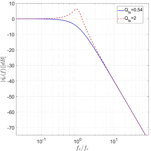
frequency dependent behaviour of the loudspeaker displace-ment. The normalized voice coil displacement for different values of Qts is shown in Figure 2. It can be noted how

the total damping affects the displacement behaviour around

fv/fr = 1, while the displacement is virtually constant at

fv/fr≤1/3 and proportional to1/fv2 atfv/fr≥3.

Figure 2: Normalized voice coil displacement, with Qts =

0.54(blue line) and Qts= 2 (red line).

Depending on the amplitude of the displacement, the trans-ducer will generate distorted signals that can be classified as linear (low displacement amplitude) and non linear (high displacement amplitude) distortion. Both of them are regarded as regular distortions because they are accepted within the design process and are results of optimization process giving the best compromise with other constraints (weight, cost, size). On the other hand, irregular distortions are non acceptable defects in a loudspeaker passing the EOL tests. They are generated by defects caused during the manufacturing process, ageing and other external factor such as overload and tem-perature. A rubbing voice coil, buzzing parts, loose particles and air leaks are typical loudspeaker defects which produce irregular distortion, quite audible and not acceptable, generally defined as “rub & buzz”. In a woofer, for example, at higher frequencies (e.g. above 1kHz), the cone itself is not rigid and should be modelled as a flexible system. The vibrations travel transversally along the cone surface in what is generally referred to as cone break up. This behaviour generally becomes a dominant factor when the wavelength of the sound in air is comparable to or less than twice cone diameter [2], [3]. Above this frequency, radial and rocking modes are natural vibration patterns of the membrane, producing non linear or undesired output. Furthermore, the presence of any irregularities (e.g. mass distribution) produced in the manufacturing/assembling

process, and/or diaphragms subjected to asymmetric acoustic loads enhance this phenomena. This becomes even more critical in small drivers such as headphones or micro-speakers, where small irregularities in the stiffness, mass and magnetic field distributions can affect dramatically the dynamic be-haviour of these tiny structures [3], [14], [15]. The resulting distortion depends highly on the amplitude and type of the stimulus. A well known technique commonly used in audio environment to completely characterise the system with a single, fast and easy measurement was introduced in [16], [17], [18]. It is based on exponentially swept sine signal defined as:

x(t) = sin





2πf1T

lnf2

f1

_f

2 f1

Tt

−1

!

 (3)

whereT is the length of the sine sweep in seconds, andf1

andf2 the starting and ending frequencies, respectively. This

technique has the ability to separate the non-linear (distortion) responses from the linear response of the system. When the measured signal y(t)is convolved with an inverse filterg(t), namely the time reversal version of the test signalx(t), the linear response compresses to an almost perfect impulse, with a delay equal to the length of the test signal. Simultaneously, the harmonic distortion responses compress to other smaller impulses, located at precise time delays occurring earlier than the impulse response. Applying a suitable time window it is possible to extract just the portion required, containing only the linear response or the distortion products. Thus, a Fourier transform can be applied, and both linear and non linear (harmonics) frequency responses can be displayed.

Having briefly introduced some of the aspects of the electrody-namic transducer motion, and how to acoustically characterize the behaviour of a speaker, further experimental analysis will be shown in the next sections focusing mainly on the rigid body motion of the loudspeaker at low frequencies in order to detect, confirm and characterize its behaviour through radar micro-Doppler signature.

III. MICRO-DOPPLERANALYSIS

An operating loudspeaker present a complex scenario of moving parts which can generate a multifaceted pattern of vibrations. Radar sensor can be used to identify the vibration pattern of the transducer. To fully understand and interpret correctly the radar micro-Doppler phenomena in complex and realistic scenario, the basics of the micro-Doppler will be introduced in Section III-A where the single tone signal is used as stimulus, while in Section III-B the micro-Doppler signature of a speaker playing the exponential sine sweep in (3) is analysed. Finally, in Section III-C the radar based mechanical characterization of the speaker will be introduced. For all these analyses, a sampling frequency fs = 22kHz is

considered.

A. Single tone Analysis

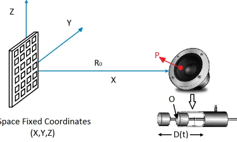
a target. Thus, the Doppler frequency shift, rapresenting the change of phase function over time, can be used to detect vibrations or rotations of structures in a target. In Figure 3 the geometry used to analyse the micro-Doppler induced by a vibrating target is shown [4], [5].

Figure 3: Geometry for the radar and generic vibrating point: the motion of a speaker can be described as rigid body motion having a piston mode when the input to the loudspeaker is a signal with frequency range up to1kHz.

The receiving Doppler from a target as a function of time is modelled as follows:

sr(t) =ρexp{j[2πf0t+ Φ (t)]} (4)

where ρ is the reflectivity of the vibrating point scatterer,

f0is the carrier frequency of the transmitted signal and Φ (t)

is the time varying phase change of the vibrating scatterer. LettingR0be the distance between the radar and the speaker’s

initial positionO, then the range function varies with time due to the speaker micro-motion:

R(t) =R0+D(t) (5)

Assuming an arbitrary point of the cone located in P

vibrates with sinusoidal frequencyfv and maximum

displace-ment η˜c(fv), the displacement function will be of the kind:

D(t) = ˜ηc(fv) sin (2πfvt) (6)

while assuming the radar being in the line of the sight with the speaker [4], [5]. Then, the time varying phase can be written as:

Φ (t) =βR(t) =β[R0+ ˜ηc(fv) sin (2πfvt)] (7)

where

β= 4π

λ (8)

withλthe wavelength of the transmitted signal. Substituting (7) in (4) the received signal can be expressed as [12]:

sr(t) =ρexp

j4πR0

λ

exp

j2πf0t+j

4πη˜c(fv)

λ sin (ωvt)

(9)

where ωv = 2πfv. In order to simulate a received radar

signal, the backscattering coefficient ρ[4], [5] relative to the only vibrating metallic component, namely the voice coil, is modelled as flat circular plate and calculated as:

ρ= 4π 3_r4

λ2 (10)

with λthe radar signal wavelength and r is the radius of voice coil. From (9), the derivative of the second phase term leads to the expression of the micro-Doppler shift:

fmD(t) =

1 2π

dΦ dt =

4π

λη˜c(fv)fvcos (2πfvt) (11)

In Figure 4 the theoretical micro Doppler of a speaker moving at its resonance frequency of 67Hz, with output voltage of 5V and10V, is shown.

Figure 4: Theoretical micro Doppler of a speaker moving at its resonance frequency offv =fr = 67Hz with output voltage

of 5V and10V, modelled as a flat circular plate having max-imum displacement ofη˜c,5V = 1.1mm andη˜c,10V = 2.2mm.

From (1), the theoretical displacement η˜c at 5V and 10V

of output voltage is computed. With a η˜c,5V = 1.1mm and

˜

ηc,10V = 2.2mm, the maximum Doppler shift achievable is

73.90Hz and147.80Hz, respectively.

Figure 5: Normalised spectrum of the simulated received signal of a speaker moving at its resonance frequency of

fv = 67Hz with output voltage of 5V and 10V, modelled

as a flat circular plate having maximum displacement of

˜

ηc,5V = 1.1mm andη˜c,10V = 2.2mm.

amplitude increases, particularly at low frequencies, the most dominant non linearities effects are introduced by stiffness

Kms(˜ηc)(reciprocal of the complianceCms(˜ηc)), force factor

Bl(˜ηc) and inductanceLe(˜ηc), function of the displacement

˜

ηc. A second non linear effect is the generation of additional

spectral components which are not in the exciting stimulus; these components are generally multiple of the fundamental frequency and thus labelled as harmonic and intermodulations distortion[3].

From this simple set of equations in (7),(9) and (11) describing the micro-Doppler signature we can deduct the capability to retrieve information about the behaviour, anomalies and failures of a loudspeaker from the radar returned.

While the spectral composition of a signal varies as function of the time, the conventional Fourier transform cannot provide a time dependent spectral description. Thus, a joint frequency distribution provides more insight into the time-varying behaviour of the signal. The squared magnitude of the Short-Time Fourier Transform [6], [8] of the received radar signal, namely the spectrogram χ(ν, κ), is used to examine the time-frequency distribution as:

χ(ν, κ) =|ST F T{sr(n)}|

2

=

N−1

X

n=0

sr(n)h(n−κ) exp(

−j2πνn

N )

2

(12)

whereκ= 0. . . , K−1,ν is the normalised frequency and

h(n)is a discrete window function of choice [7], [11]. In Figure 6, spectrograms of the simulated received radar signal of a speaker moving at its resonance frequency fv =

(a) Blackman-Harris window of11.6ms

(b) Blackman-Harris window of23.2ms

Figure 6: Magnitude square of the spectrogram of the sim-ulated received radar signal from a speaker moving at its resonance frequency fv = fr = 67Hz with output voltage

of 5V, modelled as a flat circular plate having maximum displacement η˜c,5V = 1.1mm. The maximum Doppler shift

is highlighted with a black line.

fr= 67Hz with output voltage of5V are shown. For a better

Figure 7: Magnitude square of the spectrogram of the sim-ulated received radar signal from a speaker moving at its resonance frequency fv = fr = 67Hz with output voltage

of 10V, modelled as a flat circular plate having maximum displacementη˜c,10V = 2.2mm, with Blackman-Harris window

of 5.8ms. The maximum Doppler shift is highlighted with a black line.

spectrogram in Figure 7 reveals a maximum Doppler shift of

150Hz, in agreement with what is expected from theory in (11).

B. Sine Sweep Analysis

Using the chirp signal x(t)in (3), the ideal received radar signalsr(t)in baseband is modelled as:

sr(t) =ρexp

j4πη˜c(fv(t)) λ x(t)

(13)

with the displacement η˜c be a time varying function of

fv(t), as described in (1). For an exponential sine sweep, the

instantaneous vibration frequency fv(t)is defined as:

fv(t) =f1kt=f1

_f

2 f1

Tt

(14)

with k the exponential chirp rate. Depending on the be-haviour of the displacement, the micro Doppler will show a different envelope, strictly related to voice coil motion. In case of constant displacement η˜c during the sweep, the maximum

micro Doppler increases linearly with the frequency of the stimulus, with fixed modulation index Υ = βη˜c, as in (11).

In Figure 8 the maximum micro Doppler for different fixed displacement at different vibration frequencies are shown.

Considering a fixed displacement η˜c = 10mm with an

exponential chirp of T = 60 seconds long in the frequency band fv ∈ [20,1000]Hz, the theoretical maximum

micro-Doppler shift achievable is 10kHz. The spectrogram of the simulated received radar signal is shown in Figure 9.

Figure 8: Theoretical micro Doppler for different displacement

˜

ηc at different vibration frequencies fv, with a fixed

wave-length λ= 1.25cm.

Figure 9: Magnitude square of the simulated spectrogram of an ideal received radar signal from a speaker playing aT = 60

seconds exponential sine sweep withfv ∈[20,1000]Hz, with

fixed displacement equal η˜c= 10mm.

Then, it is necessary consider both displacement and vibration frequency as function of the time. With this assumption the theoretical micro Doppler equation will become the sum of two components, namely:

fmD(t) =

2 λ

dη˜c(t)

dt x(t) +

4πfv(t)

λ η˜c(t) dx(t)

dt (15)

Let’s consider a loudspeaker with resonance frequency

fr = 67.50Hz, playing an exponential sine sweep of length

T = 60 seconds, with instantaneous vibration frequency

fv ∈[20,5000]Hz. In the hypotheses of initial displacement

˜

ηc(t = 0) = 2.26cm, related to initial vibration frequency

fv(t= 0) = 20Hz, the theoretical micro Doppler frequency is

computed by equation (15) and shown in Figure 10.

Figure 10: Theoretical micro-Doppler frequency shift from of a speaker playing an exponential sine sweep of T = 60s, withfv∈[20,5000]Hz, and initial displacement η˜c(t= 0) =

2.26cm andfv(t= 0) = 20Hz.

Unlike the constant displacement scenario, the micro Doppler frequency achieves its maximum valuefmD= 887Hz

at the time instanttmax= 13.2305s, namely the instant which

the vibration frequency fv matches the resonance frequency

fr of the speaker itself. As expected, this suggests that the

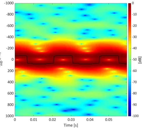
highest micro Doppler shift is achieved at the highest velocity of the speaker, namely at the resonance frequency. Notice that at high vibration frequency, the micro Doppler tends towards zero due to the displacement function. The spectrogram of the simulated received radar signal has shown in Figure 11, where a Blackman-Harris window of 46.5ms is used.

From Figure 11 the behaviour of the micro Doppler fre-quency is confirmed. While the sinusoidal like motion of the micro Doppler is still visible at low vibration frequency achieving the maximum value at the resonance frequency, at high vibration frequency it is clear the strong component at the zero frequency. The spectrogram of a time window of0.05s of

Figure 11: Magnitude square of the spectrogram of the simu-lated received radar signal from a speaker playing an exponen-tial sine sweep ofT = 60s, withfv∈[20,5000]Hz, and initial

displacementη˜c(t= 0) = 2.26cm and fv(t= 0) = 20Hz.

the simulated received radar signal around tmax is shown in

Figure 12, confirming the sinusoidal like motion of the micro Doppler.

Figure 12: Magnitude square of the spectrogram of time win-dow of0.05s of the simulated received radar signal around the time instanttmax, where Doppler shift achieves its maximum,

namely in proximity of the resonance frequency fr of the

speaker. The maximum Doppler shift is highlighted with a black line.

target. So the speaker vibration can then introduce an infinite series of paired echoes m because, when considering (15), the received signalsr in (13) may be expressed as a series of

expansion of Bessel functions of the first kind of order m:

Jm

_4πη˜

c

λ

= 1 2π

Z +π

−π

exp

j

_4πη˜

c

λ sin (u)−mu

du

(16) such that the received radar signal sr in baseband can be

expressed as:

sr(t) =ρexp

j4πR0

λ

exp{j2πf0t}

+∞

X

m=−∞

Jm

_4πη˜

c

λ

exp

mj2πf1(k

t₋₁₎

logk

=

ρexp

j4πR0

λ

exp{j2πf0t}

J0

_4πη˜

c

λ

+

+J1

_4πη˜

c

λ

exp

j2πf1(k

t₋₁₎

logk

+

−J1

_4πη˜

c

λ

exp

−j2πf1(k

t₋₁₎

logk

+

+J2

_4πη˜

c

λ

exp

j4πf1(k

t₋₁₎

logk

+

−J2

_4πη˜

c

λ

exp

−j4πf1(k

t₋₁₎

logk

+. . .

(17)

with k the exponential chirp rate. Therefore, the micro-Doppler frequency spectrum consists of pairs of spectral lines around the center frequency f0 and with spacingfv between

adjacent lines. The intensity of paired echoes visible depends from the modulation index Υ = βη˜c. In case of wideband

modulation (Υ>1) more spectral lines appear. This is visible in the spectrograms in Figure 9 where, a fixed displacement of 10mm makes the signal wideband modulated with fixed modulation index: multiple and very densely spaced paired echoes are introduced. Due to a non constant displacement, a different behaviour is shown through the spectrogram in figure 11 where the received signal will be wideband modulated at low vibrational frequency and narrowband modulated at high vibrational frequency. Thus, more harmonics are detected at low vibration frequencies. This results is in agreement with loudspeaker modelling theory, where the harmonics compo-nents at low vibration frequencies are defined as regular non linear distortions components, generated by the non linear behaviour of stiffness, force factor and inductance of the driver.

C. Mechanical Characterization of a Speaker

The ability of the radar technology to detect the motion of a speaker has been described above. When a chirp is used in the simulated scenario, the voltage as the force factor is supposed to be constant with the frequency of the stimulus. In a real scenario this hypothesis is not justified due to the non linearities, introduced for example by stiffness (Kms(˜ηc)),

force factor (Bl(˜ηc)) and inductance (Le(˜ηc)). To understand

the influence of the non linearities on the speaker behaviour, in terms of deviation from the ideal piston mode behaviour,

an alternative approach is considered. Commonly used in radar is the matched filter technique, obtained by correlating a known signal with an unknown signal to detect the presence of the template in the unknown signal. This is the radar equivalent of the acoustic measurement technique introduced in [16], [17], [18], where the unknown signal is convolved with a conjugated time-reversed version of the template. With this technique the speaker can be mechanically characterized. The matched filter is the optimal linear filter for maximizing the signal-to-noise ratio (SNR) in the presence of additive stochastic noise. If the model of the ideal received radar signal is found, matched filter technique could be applied to RF sensors in order to characterize the mechanical behaviour of the speaker. Using (13) the received radar signal in baseband of an ideal loudspeaker, behaving as piston mode in the full frequency band, is described. It can be seen as the product between the magnitude and phase components. While the phase component depends on both T&S parameters of the speaker and the stimulus waveform, the magnitude component introduces uncertainty since it is an estimation of the target reflectivity, which is usually difficult to estimate. For this reason, to reduced the amount of uncertainty, the system’s impulse response can be computed by simply correlating the phase of the measured radar signaly(t)with the phase of the simulated signalsr(t), such that:

h(t) =_∠y(t)?_∠sr(t). (18)

where? is the correlation operator. With an exponential sine sweep of T = 60 seconds long as a test signal, and with the hypothesis of a linear system, the results would be a perfect peak centred in T, defined as linear impulse response, as shown in the Figure 13.

Figure 13: Matched filter output of the simulated radar signal from an ideal speaker, playing an exponential sine sweep of

In a real scenario instead, where the Device Under Test (DUT) is never linear, along with the linear impulse responses, non linear impulse responses are also obtained, corresponding to the various harmonics of the input signal. With the exponen-tial sine sweep, these non linear product, do not contaminate the linear impulse response, as they are occurring at very precise anticipatory times ∆t before the linear response, namely:

∆t=T ln (N) lnf2

f1

(19)

where N is the N thdistortion component. Thus, the signal component of the time waveform at the output of the matched filter is actually the autocorrelation functionrsr,sr of the ideal

signal. The matched filter peakh(T)is thenrsr,sr(0) =Esr,

whereEsr is the total energy in the signalsr(t)[19].

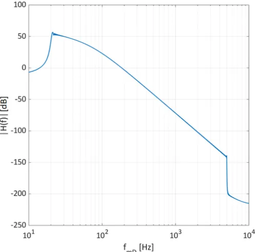
Apply-ing a window around the peakh(T), it is possible to compute the linear frequency response through Fourier Transform. In the event where no window is applied, the Power Spectral Density (PSD) of the signal is computed, where the harmonic components and noise are incorporated into the frequency response. In Figure 14 the PSD of the simulated radar signal from an ideal speaker is shown.

Figure 14: Normalised frequency responses of an ideal speaker, playing a exponential sine sweep of T = 60s with

fv∈[20,5000]Hz.

Later in this paper, the harmonic distortion responses will not be discarded but analysed. The system’s response is affected in varying ways by different irregular defects, mak-ing the non-linear behaviour of the loudspeaker vibrations a powerful indicator of possible manufacturing problems. Thus, in the real scenario it is possible to define the time waveform at the output of the matched filter as the cross correlation functionry,sr between the measured signaly(t)and the ideal

Parameter Value

fr 67.57Hz Bl 9.67N/A Qts 0.5425 Qes 0.6075

Table I: Measured Thiele&Small Parameters ofB&C 10CL51

LF driver.

one sr(t), where its Fourier Transform is referred as Cross

Power Spectrum Density (CPSD).

IV. REAL MEASUREMENT ANALYSIS

In this section, real data acquisitions are analysed and compared with simulation results. In Section IV-A, the micro-Doppler signature is analysed considering a single tone acous-tic signal. The micro-Doppler signature of a speaker playing a sine sweep is analysed in Section IV-B. Finally, in Section IV-C the mechanical characterization of a real speaker is shown. For all of the analyses, the signal amplitude was set to −6dB for the standard “Loudness units relative to Full Scale” (LUFS) to prevent any digital or analog clipping in the measurement chain. In order to simulate a received radar signal, a diameter of 25cm (which is a typical dimension for a loudspeaker operating in this frequency range) has been considered. The backscattering coefficient ρ[5] coming from the only vibrating metallic component, namely the voice coil, is calculated as in (10), with the radius of voice coil

r = 2.55cm. The measurements acquisition was conducted through a bespoke 24GHz CW radar made by WhiteHorse Radar LTD. It has been used to measure the returns from a

25cm low frequency driver placed1m away from the radar on the Line Of Sight (LOS). For both simulated and real data, a sampling frequencyfs= 22kHz is considered. Through aClio

Pocketboard [20], the electromechanical parameters needed to feed the model of the ideal received radar signal are computed. The measured T&S parameters ofB&C 10CL51LF driver [21] are reported in Table I.

In Figure 15, the system set up is shown. The input signal to the loudspeaker has been generated byAdobe Audition 3.0, while the received signal is acquired by the radar through

Matlab R2018a, also used to process the data.

A. Micro Doppler Signature: Single tone analysis

In this section, the single tone analysis is performed, where real data are analysed and compared to simulation results. A single tone has been chosen as acoustic input to the loudspeaker with frequency fv = 67Hz to drive an ideally

flat and rigid disk behaving in piston mode, at its resonance frequency. To understand the ability of the radar to detect the motion of the speaker, two different output voltage were be taken in consideration. Setting the voltage at the loudspeaker terminals to be 5V, the normalized spectrum of the received signal is shown in Figure 16.

Figure 15: Experiment Setup.

Figure 16: Spectrum of real radar measurement from a 25cm loudspeaker playing a single tone fv= 67Hz at its resonance

frequency at5V output voltage.

Although the presence of the noise floor, the fundamental component and its harmonics are visible and in agreement with the spectrum of the simulated signal. The discrepancy between the ideal and the real spectrum is related to the non linear effect of the DUT, previously defined. Moreover, the discrepancy between the positive (blue curve) and negative direction (red curve) may be related to the effect of non linear

stiffness. In Figure 17, a Blackman-Harris window of23.2ms long is used to generate the spectrogram of the radar signal.

Figure 17: Magnitude square of the spectrogram of real radar measurement from a 25cm loudspeaker playing fv = 67Hz

single tone at 5V output voltage, with Blackman-Harris win-dow of 23.2ms. The maximum Doppler shift is highlighted with a black line.

From the spectrogram the maximum frequency Doppler shift can be evaluated and from this the displacement. Inverting (11), the maximum value ofη˜c,5V can be obtained. As in the

simulated scenario (in Figure 6(b)), the micro Doppler has a maximum value equal to 75Hz, in both positive and negative direction, leading to the estimation of the displacement equal to1.1mm. In the case of an output voltage of10V, the speaker should be more prone to distortion. This is visible from the spectrum shown in Figure 18, where harmonics with higher magnitude appear due to a larger displacement are visible from the spectrogram in Figure 19.

Although the behaviour is still in agreement with the model in Figure 7, some discrepancies appear. The differences with the ideal micro Doppler are illustrated in Figure 20.

While in the simulated scenario the micro Doppler profile has a maximum and minimum value equal to 150Hz, the measured one resulted to be 150Hz in the positive direction and172Hz in the negative direction. This suggests that, due to non linear effects, the voice coil is susceptible to acceleration in order to reach the farthest point from the radar, visible through the different rising and falling front from the simulated one. This can be confirmed by the phase of the signal.

In Figure 21 and 22 the phase of the real and simulated radar signals are compared when an output voltage is set to

5V and 10V, respectively. It can be seen that the phase of the real data matches the simulated one in terms of sinusoidal-like motion, especially when the applied voltage is 5V. However discrepancies between the simulated and real data appear at

Figure 18: Spectrum of real radar measurement from a 25cm loudspeaker playing a single tone fv= 67Hz at its resonance

frequency at10V output voltage.

Figure 19: Magnitude square of the spectrogram of real radar measurement from a 25cm loudspeaker playing fv = 67Hz

single tone at 10V output voltage, with Blackman-Harris window of5.8ms. The maximum Doppler shift is highlighted with a black line.

simulated one, it is possible to observe that actual motion does not match completely the ideal one. From the plot it is possible to infer that the voice coil spends more time in the position further away from the radar than the piston model suggests. A possible explanation of this phenomenon could be the superposition of two components. The first is the

Figure 20: Micro Doppler comparison between the simulated signal and the real radar measurement from a 25cm loud-speaker playing67Hz single tone at10V output voltage, with Blackman-Harris window of5.8ms.

Figure 21: Comparison between the phase of the simulated and real radar signal of the speaker playing tonefv = 67Hz

equal at its resonance frequencyfr, with output voltage set to

5V.

Figure 22: Comparison between the phase of the simulated and real radar signal of the speaker playing tone fv = 67Hz

equal at its resonance frequencyfr, with output voltage set to

10V.

high displacement the suspension responds with more force than the predicted one. The second component could derive from the non linearity introduced by the force generated by the magnetic field times the length of the voice coil immersed in the gap: if the coil windings leave the gap, the force factor decreases [3]. Consequently, the non linearities appear and the coil is pushed back by magnetic field, from the nearest to the furthest position from the radar, earlier than its ideal one.

B. Micro Doppler Signature: Sine Sweep Analysis

In this section the micro Doppler signature of a speaker playing a sine sweep will be analysed and compared to the simulation results. The acoustic tone varies from a starting frequency f1= 20Hz at timet = 0, ending at the time T = 60s with frequencyf2= 5kHz. The speaker was connected to

an amplifier, which output was set toe˜g= 3V at1kHz. With

the speaker parameters in Table I, the theoretical displacement is modelled through (1): at timet= 0the maximum value of

˜

ηc = 1.1mm is found. The spectrograms of both simulated

and real radar signal are compared and shown in Figure 23. Both the spectrograms are produced using a Blackman-Harris window of46.5ms, with an overlap of 99%, with column based normalization.

The first difference that can be immediately noted, it is the presence of the noise floor. While the simulated signal has been generated in absence of noise, the real one shows a background noise increasing with time. This result is in agreement with radar sensitivity, shown in Table II: as a vibration amplitude of a micron results in a phase shift of only0.06 deg, it is almost undetectable.

(a) Spectrogram Simulated Signal

(b) Spectrogram Real Signal

Figure 23: Magnitude square of the spectrogram of simulated and real received radar signal from a speaker playing an expo-nential chirp, with T&S parameter of Table I, with Blackman-Harris window of46.5ms.

It can be seen in Figure 23b that a high intensity distortion is visible at the time instantt= 42s, with vibration frequencyfv

Vibration Amplitude Maximum Phase Shift

1cm 576 deg

1mm 58 deg

1µm 0.06 deg

Table II: Sensitivity of a24GHz CW radar to different vibra-tion amplitude.

to create a larger amplitude wave. If they meet in such a way that their displacements are exactly opposite (180 degrees out of phase), then the wave energies will cancel each other. At phase angles between 0 degrees and 180 degrees, there will be a range of intermediate stages between full addition and full cancellation. Using the mathematical formulation in (15), the theoretical micro Doppler related to the theoretical displacement is shown in Figure 24.

Figure 24: Theoretical micro Doppler frequency shift of a speaker playing a 60 seconds exponential sine sweep with

fv∈[20,5000]Hz, with T&S parameter of Table I.

Also in this case the maximum Doppler shift happens at the resonance frequency of the speaker, with maximum value of fmDM AX = 44.3Hz at the time tmax = 13.23s. The

spectrograms of both simulated and real radar signal around

tmax are shown in Figure 25

From the spectrograms in Figure 25 is possible to appreciate how the simulated signal matches with the real measurement. In both the spectrograms, a maximum Doppler shift of107Hz is detected with a Blackman-Harris window of 11.6ms. Due to both the spectrogram time-frequency dilemma and coupled echoes phenomenon, the maximum Doppler shift detected dif-fers from the theoretical one making the echoes stronger than the main component. Thus, for a correct characterization of the speaker, an alternative approach is needed and introduced in the next section.

(a) Spectrogram Simulated Signal

(b) Spectrogram Real Signal

Figure 25: Magnitude square of the spectrogram of simulated and real received radar signal from a speaker playing an exponential chirp, with T&S parameter of Table I, at the

t = tmax and fv = fr, with Blackman-Harris window of

11.6ms.

C. Mechanical Characterization of a speaker

linear impulse response. Real devices unfortunately are never linear; thus, not only a linear impulse response appears, but also non linear impulse responses are obtained, corresponding to the various harmonics of the input signal. This is visible in the Figure 26, where the matched filter is applied to a real measurement.

Figure 26: Matched filter output: linear and non linear impulse responses of the DUT, with measured T&S parameters of table I.

In agreement with (19), the non linear products occur at very precise anticipatory time before the linear response, namely at ∆t2nd = 7.50s, ∆t3rd = 11.93s and ∆t4th = 15.04s.

Applying a Fourier Transform to the matched filter output, the frequency response of the DUT can be evaluated. In Figure 27, CPSD, linear and harmonic frequency responses are shown.

In case of no windowing, the CPSD of the signal is com-puted in Figure 27 (blue line) where harmonics products and noise are incorporated into the frequency response. Applying a window around the peak in h(T), the linear frequency response can be assessed. Since the non linear products are a powerful indicator of possible manufacturing problems, they are analysed too. For this reason, windows are applied to harmonic responses as well. As it can be noted from the Figure 27, the harmonic products affect the behaviour of the speaker mainly at low frequency, where the device is more susceptible to the non linear effects, in agreement with loudspeaker model theory.

V. CONCLUSION

In this paper a novel approach based on radar micro Doppler has been proposed for condition monitoring of loudspeakers in hostile environments. With the assumption of rigid body motion at low frequency, the displacement of a loudspeaker has been modelled as function of the frequency of the stimulus by

Figure 27: CPSD, linear frequency response and harmonic fre-quency responses of the DUT, with measured T&S parameters of table I.

VI. ACKNOWLEDGEMENT

This work was supported by the Engineering and Phys-ical Sciences Research Council (EPSRC) Grant number EP/K014307/1 and the MOD University Defence Research Collaboration in Signal Processing.

REFERENCES

[1] W. Klippel, “Scanning Vibrometer C5 Hardware and Software Module of the KLIPPEL R&D SYSTEM,” Klippel GmbH, Mendelssohnallee 30, 01309 Dresden, Germany, Tech. Rep., 2008.

[2] W. Klippel and J. Schlechter, “Measurement and visualization of loudspeaker cone vibration,” inAudio Engineering Society Convention 121, Oct 2006. [Online]. Available: http://www.aes.org/e-lib/browse. cfm?elib=13716

[3] W. Klippel, “Tutorial: Loudspeaker nonlinearities - causes, parameters, symptoms,”Journal of Audio Engineering Society, vol. 54, no. 10, pp. 907–939, 2006. [Online]. Available: http://www.aes.org/e-lib/browse. cfm?elib=13881

[4] V. C. Chen,The Micro-Doppler Effect in Radar. Artech House, 2011. [5] C. Clemente, A. Balleri, K. Woodbridge, and J. J. Soraghan, “Developments in target micro-doppler signatures analysis: radar imaging, ultrasound and through-the-wall radar,”EURASIP Journal on Advances in Signal Processing, vol. 2013, no. 1, p. 47, Mar 2013. [Online]. Available: https://doi.org/10.1186/1687-6180-2013-47 [6] D. Gaglione, C. Clemente, F. K. Coutts, G. Li, and J. J. Soraghan,

“Model-based sparse recovery method for automatic classification of helicopters,” in2015 IEEE Radar Conference (RadarCon), May 2015, pp. 1161–1165.

[7] C. Clemente, L. Pallotta, A. D. Maio, J. J. Soraghan, and A. Farina, “A novel algorithm for radar classification based on doppler characteristics exploiting orthogonal pseudo-zernike polynomials,”IEEE Transactions on Aerospace and Electronic Systems, vol. 51, no. 1, pp. 417–430, January 2015.

[8] R. I. A. Harmanny, J. J. M. de Wit, and G. P. Cabic, “Radar micro-doppler feature extraction using the spectrogram and the cepstrogram,” in2014 11th European Radar Conference, Oct 2014, pp. 165–168. [9] A. R. Persico, C. Clemente, D. Gaglione, C. V. Ilioudis, J. Cao, L.

Pal-lotta, A. D. Maio, I. Proudler, and J. J. Soraghan, “On model, algorithms, and experiment for micro-doppler-based recognition of ballistic targets,”

IEEE Transactions on Aerospace and Electronic Systems, vol. 53, no. 3, pp. 1088–1108, June 2017.

[10] Y. Kim, S. Choudhury, and H. Kong, “Application of micro-doppler signatures for estimation of total energy expenditure in humans for walking/running activities,”IEEE Access, vol. 4, pp. 1560–1569, 2016. [11] A. Assmann, A. Izzo, and C. Clemente, “Efficient micro-doppler based pedestrian activity classification for adas systems using krawtchouk moments,” in 11th International Conference on Mathematics in Signal Processing (IMA), Dec 2016. [Online]. Available: https: //strathprints.strath.ac.uk/id/eprint/66617

[12] A. Izzo, L. Ausiello, C. Clemente, and J. J. Soraghan, “Radar micro-doppler for loudspeaker analysis: An industrial process application,” pp. 1–6, Oct 2017.

[13] L. L. Beranek and T. J. Mellow, “Chapter 6 - electrodynamic loudspeakers,” in Acoustics: Sound Fields and Transducers, L. L. Beranek and T. J. Mellow, Eds. Academic Press, 2012, pp. 241– 288. [Online]. Available: http://www.sciencedirect.com/science/article/ pii/B9780123914217000063

[14] G. Ni and S. J. Elliott, “Wave interpretation of numerical results for the vibration in thin conical shells,”Journal of Sound and Vibration, vol. 333, no. 10, pp. 2750–2758, May 2014. [Online]. Available: https://eprints.soton.ac.uk/364781/

[15] W. . Klippel and J. Schlechter, “Distributed mechanical parameters describing vibration and sound radiation of loudspeaker drive units,” in Audio Engineering Society Convention 125, Oct 2008. [Online]. Available: http://www.aes.org/e-lib/browse.cfm?elib=14683

[16] A. Farina, “Simultaneous measurement of impulse response and distortion with a swept-sine technique,” inAudio Engineering Society Convention 108, Feb 2000. [Online]. Available: http://www.aes.org/ e-lib/browse.cfm?elib=10211

[17] A. Farina, “Advancements in impulse response measurements by sine sweeps,” in Audio Engineering Society Convention 122, May 2007. [Online]. Available: http://www.aes.org/e-lib/browse.cfm?elib=14106

[18] M. C. Bellini, L. Collini, A. Farina, D. Pinardi, and K. Riabova, “Measurement of loudspeakers with a laser doppler vibrometer and the exponential sine sweep excitation technique,” Journal of Audio Engineering Society, vol. 65, no. 7/8, pp. 600–612, 2017. [Online]. Available: http://www.aes.org/e-lib/browse.cfm?elib=19175

[19] M. A. Richards, J. A. Scheer, and W. A. Holm, Principles of Modern Radar, ser. Principles of Modern Radar. SciTech Publishing, Incorporated, 2010, no. v. 1. [Online]. Available: https: //books.google.it/books?id=nD7tGAAACAAJ

[20] Audiomatica S.r.l., “Clio poket 2.0,” 2001, http://www.audiomatica.com/ wp/?page id=2429.