Development and Validation of a Thermo-Economic Model for Design Optimisation and Off-Design Performance Evaluation of a Pure Solar Microturbine

(1)

City, University of London Institutional Repository

Citation:

Iaria, D., Nipkey, H., Al Zaili, J., Sayma, A. I. ORCID: 0000-0003-2315-0004 and

Assadi, M. (2018). Development and Validation of a Thermo-Economic Model for Design

Optimisation and Off-Design Performance Evaluation of a Pure Solar Microturbine. Energies,

11(11), 3199.. doi: 10.3390/en11113199

This is the published version of the paper.

This version of the publication may differ from the final published

version.

Permanent repository link:

http://openaccess.city.ac.uk/21247/

Link to published version:

http://dx.doi.org/10.3390/en11113199

Copyright and reuse: City Research Online aims to make research

outputs of City, University of London available to a wider audience.

Copyright and Moral Rights remain with the author(s) and/or copyright

holders. URLs from City Research Online may be freely distributed and

linked to.

(2)

energies

Article

Development and Validation of a Thermo-Economic

Model for Design Optimisation and Off-Design

Performance Evaluation of a Pure Solar Microturbine

Davide Iaria1,_{*, Homam Nipkey}2 _{, Jafar Al Zaili}1_{, Abdulnaser Ibrahim Sayma}1_and Mohsen Assadi2

1 _{Department of Mechanical Engineering & Aeronautics, School of Mathematics, Computer Science &} Engineering, University of London, London EC1V 0HB, UK; [email protected] (J.A.Z.);

[email protected] (A.I.S.)

2 _{Institutt for energi-og petroleumsteknologi, Stavanger University, 4036 Stavanger, Norway;} [email protected] (H.N.); [email protected] (M.A.)

* Correspondence: [email protected]; Tel.: +44-7576478587

Received: 11 October 2018; Accepted: 12 November 2018; Published: 18 November 2018

Abstract:The aim of this paper is to present a thermo-economic model of a microturbine for solar dish applications, which demonstrates the applicability and accuracy of the model for off-design performance evaluation and techno-economic optimisation purposes. The model is built using an object-oriented programming approach. Each component is represented using a class made of functions that perform a one-dimensional physical design, off-design performance analysis and the component cost evaluation. Compressor, recuperator, receiver and turbine models are presented and validated against experimental data available in literature, and each demonstrated good accuracy for a wide range of operating conditions. A 7-kWemicroturbine and solar irradiation data available for Rome between 2004 and 2005 were considered as a case study, and the thermo-economic analysis of the plant was performed to estimate the levelised cost of electricity based on the annual performance of the plant. The overall energy produced by the plant is 10,682 kWh, the capital cost has been estimated to be EUR 27,051 and, consequently, the specific cost of the plant, defined as the ratio between the cost of components and output power in design condition, has been estimated to be around EUR 3980/kWe. Results from the levelised cost of electricity (LCOE) analysis demonstrate a levelised cost of electricity of EUR 22.81/kWh considering a plant lifetime of 25 years. The results of the present case study have been compared with the results from IPSEpro 7 where the same component characteristic maps and operational strategy were considered. This comparison was aimed to verify the component matching procedure adopted for the present model. A plant sizing optimisation was then performed to determine the plant size which minimises the levelised cost of electricity. The design space of the optimisation variable is limited to the values 0.07–0.16 kg/s. Results of the optimisation demonstrate a minimum LCOE of 21.5 [EUR/kWh] for a design point mass flow rate of about 0.11 kg/s. This corresponds to an overall cost of the plant of around EUR 32,600, with a dish diameter of 9.4 m and an annual electricity production of 13,700 [kWh].

Keywords:solar dish; micro gas turbine; thermo-economic model; concentrated solar power

1. Introduction

The rapid growth of the world population, as well as the expansion of the industrial sector, has led to a continuously growing demand for electrical power. This growth, coupled with the need for reduction of greenhouse gas emissions, has created serious global challenges, e.g., achieving energy demand without violating increasingly stricter environmental regulations. This challenge has led to a

(3)

considerable push to develop clean power generation technologies. In this context, there has been a renewed interest in concentrated solar power (CSP) development.

One of the available technologies in the market is dish CSP systems. These arrangements are composed of a reflective surface, which usually has the profile of a paraboloid. The paraboloid mirrors reflect incident sunrays to a solar receiver, redirecting the sunbeams to a small region at the focal spot. The receiver absorbs the irradiated energy and convert it as heat delivered to the plant’s working fluid. A sun tracking system is usually adopted to follow the sun in all directions and maximise the annual capture of solar energy.

Parabolic dish systems boast the highest potential for solar conversion efficiencies of all the CSP technologies. The concentrator always presents its full aperture directly in the direction of the sun and avoids the optical efficiency drop due to the “cosine effect”, which usually affects other arrangements [1]. Parabolic dish CSP can operate as a stand-alone system, generating heat and/or electricity even in zones with no connection to the grid, but can also be stacked to form larger power plants in a similar fashion to photovoltaic parks with almost half the land occupancy for the same electrical output.

Parabolic dish systems, typically powering a Sterling engine, are however the least commercially mature technology among all CSP plants. One of the main issues related to Stirling engine technology is leakage of the working fluid of the power cycle, which is usually pressurised helium or hydrogen, used due to their good heat-transfer characteristics. Since the molecular weights of these gases are low, engines are designed to operate at high pressure, from 5 to 20 MPa, to maximise the power output. Another problem of these power plants is their relatively short lifetime. To make the system economically feasible, a lifetime above 20 years is required, which is far above the lifetime of Stirling engines, usually characterised by a life cycle of 10–15 year [1]. It is therefore necessary to consider the replacement of components to increase the lifetime of the system.

(4)

Energies2018,11, 3199 3 of 26

Energies 2018, 11, x FOR PEER REVIEW 3 of 27

Figure 1. OMSoP solar based MGT system [4].

CSP systems are generally designed and analysed based on the nominal design point; given the intermittence of the solar radiation, they operate for most of the time in off-design conditions. Modelling plant performance is then an important aspect for detailed analysis and design and operation optimisation. The accuracy of the models and their applicability are key aspects to consider in software development. Mazzoni et al. [7] developed a simulation tool for a pure solar dish–micro gas turbine application tailored for the OMSoP project. The set-up of the CSP plant simulator is built on a modular arrangement at the component level as presented by Cerri [8]. A library of suitable component models for the plant was realised. The simulator has been adopted to perform steady state simulations for predicting the performance under variable direct normal irradiation. The biggest advantage of the modular approach is the prospect to generate any possible plant layout and integrate new components. This characteristic creates the possibility to include the desired number of compression and expansion stages and the option to integrate any number of heat exchangers for intercooled recuperative cycles. Moreover, modularity of the tool permits an easy integration of new components, such as a combustion chamber for hybrid operations and reheating cycles or thermal storage units.

On the other hand, for optimisation purposes it is important to evaluate different plant designs considering dissimilar main cycle design parameters. To evaluate the correct size of the plant is then necessary to design and evaluate off-design performances of a wide range of possible component assembly solutions. In this situation new components must be designed. In most of the commercial software available on the market for power plant analysis, the user is often provided with a library of components to choose from, resulting in less or limited flexibility, lower applicability in terms of component selection and poor adaptability to optimisation processes.

Gavagnin et al. [6] presented a paper aimed to find the optimum design and performance of a solar micro-turbine powered by dish collectors using an innovative methodology which integrates the design and off-design models of the system, tailored over existing components of the project OMSoP. This was in contrast to the common practice of assigning an estimated efficiency to the engine turbomachinery. The design model was run for two different sets of turbine inlet temperature and recuperator effectiveness (TIT and ε): 800 °C, 85% and 900 °C, 90%. Different systems were designed for each case, yielding different off-design performance maps that link the net power output of the system to the boundary conditions of the site (ambient temperature and direct normal irradiation or DNI). With this information, annual simulations were performed in three different locations (Beijing, Seville and San Diego) based on standard performance maps for a reference DNI and on designs tailored to their particular DNI.

[image:4.595.136.462.89.272.2]

Ghavami [9] developed a computational model for pure solar dish-MGT systems. The model combines the cycle analysis of the MGT with component models to perform design point performance simulation, generate component performance maps and perform off-design

Figure 1.OMSoP solar based MGT system [4].

CSP systems are generally designed and analysed based on the nominal design point; given the intermittence of the solar radiation, they operate for most of the time in off-design conditions. Modelling plant performance is then an important aspect for detailed analysis and design and operation optimisation. The accuracy of the models and their applicability are key aspects to consider in software development. Mazzoni et al. [7] developed a simulation tool for a pure solar dish–micro gas turbine application tailored for the OMSoP project. The set-up of the CSP plant simulator is built on a modular arrangement at the component level as presented by Cerri [8]. A library of suitable component models for the plant was realised. The simulator has been adopted to perform steady state simulations for predicting the performance under variable direct normal irradiation. The biggest advantage of the modular approach is the prospect to generate any possible plant layout and integrate new components. This characteristic creates the possibility to include the desired number of compression and expansion stages and the option to integrate any number of heat exchangers for intercooled recuperative cycles. Moreover, modularity of the tool permits an easy integration of new components, such as a combustion chamber for hybrid operations and reheating cycles or thermal storage units.

On the other hand, for optimisation purposes it is important to evaluate different plant designs considering dissimilar main cycle design parameters. To evaluate the correct size of the plant is then necessary to design and evaluate off-design performances of a wide range of possible component assembly solutions. In this situation new components must be designed. In most of the commercial software available on the market for power plant analysis, the user is often provided with a library of components to choose from, resulting in less or limited flexibility, lower applicability in terms of component selection and poor adaptability to optimisation processes.

Gavagnin et al. [6] presented a paper aimed to find the optimum design and performance of a solar micro-turbine powered by dish collectors using an innovative methodology which integrates the design and off-design models of the system, tailored over existing components of the project OMSoP. This was in contrast to the common practice of assigning an estimated efficiency to the engine turbomachinery. The design model was run for two different sets of turbine inlet temperature and recuperator effectiveness (TIT andε): 800◦C, 85% and 900◦C, 90%. Different systems were designed

for each case, yielding different off-design performance maps that link the net power output of the system to the boundary conditions of the site (ambient temperature and direct normal irradiation or DNI). With this information, annual simulations were performed in three different locations (Beijing, Seville and San Diego) based on standard performance maps for a reference DNI and on designs tailored to their particular DNI.

(5)

simulation, generate component performance maps and perform off-design performance evaluation. The computational model has been coupled with an up-to-date economic model which was specifically developed through the OMSoP project for dish-MGT systems.

The approach to dish technologies has been mostly technical in the past, although for a complete assessment of a solar dish MGT power plant an economic analysis is required. More recently, Semprini et al. [10] presented a thermo-economic evaluation of a dish-MGT solar power plant during hybrid and pure solar operation. The study included a comprehensive cost analysis covering manufacturing, transportation and installation for a dish and MGT solar power generator, considering pure solar and hybrid operations. The study demonstrated that for the pure solar system, the average system purchase equipment cost, considering a production volume of 1000 units/year, was EUR 3262/kWefor the solar-only configuration and EUR 3302/kWefor the hybrid version. Regarding the dependence on MGT size, the minimum specific cost seems to be obtained for an air mass flow rate in the order of 200 g/s even if further, more refined optimisation is still needed to find the true optimal combination of size, technical specifications, layouts and configuration.

Ghavami [6] also performed a thermo-economic optimisation of a pure solar MGT. The model already described in the previous paragraph was coupled to an optimisation tool to find system designs which led to optimal thermo-economic performance for a 5-kWesystem. Then, the optimisation was extended over the rated power of 5–30 kWe to find the power rating which results in the minimum cost of generated electricity by the dish-MGT systems. To generate new performance maps of the components the model adopted scaling techniques.

Despite years of development, solar micro turbines are still in an early stage of development and needs further technological progress in order to achieve competitiveness and to be ready for a global scale commercialisation. This is especially true for the MGT dish, for which development is still at a demonstration level and, in general, the following flaws have been identified in the cited previous works in the topic:

• Low aptitude for optimisation. Most existing tools and studies are based on existing plants, resulting in reduced capability of the tool to design and evaluate accurately off-design performance of different components.

• Scarce flexibility. Most existing tools do not allow the possibility to integrate new components and consequently compare dissimilar layouts.

• Few thermo-economic assessments and optimisations concerning solar dish-MGT, and none considering integrated hybridization (fuel back-up) and/or thermal storage.

In this paper, a validated model of a microturbine for solar dish applications is presented to be used for techno-economic optimisation purposes. The aim of this study is to create a flexible and modular tool for design and off-design performance evaluation, which can be adopted for different plant layouts and operational strategies. The developed tool is not intended to be used only for optimisation purposes but can also be adopted to evaluate the performance of existing plants and components. In the first part of the paper the logic of the tool, together with the components’ models, are presented and validated. In the following results section the model is adopted for a thermo-economic assessment of a 7-kWepower plant. Finally, a plant size optimisation is presented to find the optimum size of the plant in respect of the annual power output and the component’s cost.

2. Materials and Methods

(6)

Energies2018,11, 3199 5 of 26

evaluation. Finally, a plant-size optimisation is performed to evaluate the best size of the plant that can guarantee the right trade-off between plant cost and annual power generation.

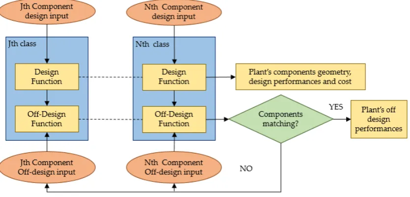
To evaluate the performance of the plant in different operational conditions, a model for each component of the plant has been developed using a modular approach. The flowchart of the model is shown in Figure2where the generic Jth module is characterised by two functions. The first is the ‘design function’ which calculates the design performance and the geometrical characteristics of the component based on the desired set of design input variables. The second is the ‘off-design function’ which evaluates the performance of the plant at off-design conditions based on the geometrical characteristics. The latter is calculated by the design function, the required set of input variables at off-design conditions and the operational strategy, for instance constant TIT. The model has been programmed using the object-oriented language C++.

The biggest advantage of the modular approach is the possibility to generate any desired plant layout. This characteristic allows the possibility of including the desired number of compression and expansion stages, the possibility to integrate any number of heat exchangers for intercooled recuperative cycles, or the possibility to integrate a combustion chamber for hybrid operations and reheating cycles.

To evaluate the performance of the plant in different operational conditions, a model for each component of the plant has been developed using a modular approach. The flowchart of the model is shown in Figure 2 where the generic jth module is characterised by two functions. The first is the

‘design function’ which calculates the design performance and the geometrical characteristics of the component based on the desired set of design input variables. The second is the ‘off-design function’ which evaluates the performance of the plant at off-design conditions based on the geometrical characteristics. The latter is calculated by the design function, the required set of input variables at off-design conditions and the operational strategy, for instance constant TIT. The model has been programmed using the object-oriented language C++.

The biggest advantage of the modular approach is the possibility to generate any desired plant layout. This characteristic allows the possibility of including the desired number of compression and expansion stages, the possibility to integrate any number of heat exchangers for intercooled recuperative cycles, or the possibility to integrate a combustion chamber for hybrid operations and reheating cycles.

Figure 2. Logic flowchart of the code.

In this study, a recuperative cycle is presented. Once the components are selected, the first calculation carried out by the software is to design the plant and its main components using design point input parameters. After the design procedure is completed, the program evaluates the off-design performance of the components based on the desired operational strategy. The off-design procedure starts by assuming a first attempt mass flow rate and iterates until all the components match each other. During iteration the matching guess is continuously updated until component matching is achieved. Further constraints can be included in the software according to the operational strategy. In this case another iteration is required and the system is solved via serial nested loops. The loops matching guesses and constraints are solved in a nested sequence until convergence.

2.1. Components Models

2.1.1. Fluid Properties Module

The fluid properties are characterised using a specific class, which can be accessed by any components’ classes. Through this module, each working fluid can be described as an object with its composition and thermodynamic properties. The specific heat of the working fluid 𝐶𝐶𝑃𝑃 as a function

[image:6.595.91.509.322.523.2]

of temperature 𝑇𝑇 is evaluated using the first order polynomial regression given in Equation (1). 𝐶𝐶𝑃𝑃=∑𝑁𝑁𝑘𝑘=1𝜇𝜇𝑘𝑘(𝐴𝐴𝑘𝑘+𝐵𝐵𝑘𝑘𝑇𝑇) (1)

Figure 2.Logic flowchart of the code.

In this study, a recuperative cycle is presented. Once the components are selected, the first calculation carried out by the software is to design the plant and its main components using design point input parameters. After the design procedure is completed, the program evaluates the off-design performance of the components based on the desired operational strategy. The off-design procedure starts by assuming a first attempt mass flow rate and iterates until all the components match each other. During iteration the matching guess is continuously updated until component matching is achieved. Further constraints can be included in the software according to the operational strategy. In this case another iteration is required and the system is solved via serial nested loops. The loops matching guesses and constraints are solved in a nested sequence until convergence.

2.1. Components Models

2.1.1. Fluid Properties Module

(7)

composition and thermodynamic properties. The specific heat of the working fluidCPas a function of temperatureTis evaluated using the first order polynomial regression given in Equation (1).

CP=

∑

N

k=1µk(Ak+BkT) (1)

whereAandBare two coefficients characteristic of the single componentkandµis the mass fraction

of the component k. Nis the total number of the constituents of the fluid. To evaluate thermal conductivity and viscosity, for the purpose of this study, the class was calibrated to consider dry air as the working fluid, using a second order interpolation of the known properties of air as a function of the temperature [11]. The effect of pressure is negligible and hence was not considered.

2.1.2. Microturbine

The MGT is modelled by its three main components: the compressor, the recuperator and the turbine. Typically, for MGT applications, centrifugal compressors are adopted. This is mainly due to their robustness for the range of mass flow rates and pressures in which MGTs operate. Additionally, a previous study conducted by the authors demonstrated that an optimised design that utilises a vaneless diffuser can lead to a wider range of operation with relatively high efficiency compared to vaned diffuser designs [12]. Hence, a centrifugal compressor design with stationary casing, impeller, stationary vaneless diffuser and volute has been adopted for this study. The design and off-design performance evaluation have been performed using a one-dimensional model based on mass, momentum and energy conservation principles as given in Equations (2) and (3).

.

m=ρinπ

R2_in,t−R2_in,hCa,in=2πRoutboutCa,outρout (2)

T0,out=T0,in

p0,out

p0,in

γ−_γ1∗_η1_pc

(3)

In Equation (2),Ris the radius,bis the blade width,ρis the density andCais the axial component of the absolute velocity. The subscriptstandhrefer to the inlet hub and tip. In Equation (3),T0andp0 are the total temperature and pressure,ηpcis the polytrophic compressor efficiency andγthe specific

heats ratio. In both equations, the suffixesinandoutrefer to the inlet and outlet, respectively. The efficiency of the compressor was evaluated using a set of standard empirical relationships available in [13]. In the adopted loss model, two categories of losses have been modeled: external (parasitic) losses and internal losses. Internal losses include all the losses that cause a pressure drop across the main channel, such as incidence losses (∆hi), blade loading (∆hbl), skin friction (∆hs f), mixing losses (∆hml), tip clearance losses (∆hcl) and vaneless diffuser losses (∆hcd). The external losses are all those losses characterised by an enthalpy loss but not a pressure loss across the main channel. The disk friction losses (∆hd f), the leakage losses (∆hlk) and the recirculation losses (∆hrc) belong to this category. The isentropic compressor efficiency then can be calculated using Equation (4), where ∆hsis the isentropic compression enthalpy change.

η= ∆hs

−∆hi−∆hs f −∆hbl−∆hcl−∆hml−∆hvd

∆hs+∆hrc+∆hlk+∆hd f

(4)

The recuperator chosen for this study is a cross flow plate-fin heat exchanger with off-set strip fins. This arrangement has one of the highest heat transfer to volume ratios of all heat exchangers available in the market [11]. Design and off-design performances of the heat exchanger have been evaluated using theε-NTUmethod which provides a model for the effectiveness and the overall heat

transfer coefficient as given in Equation (5).

ε=1−e{

1

χNTU

0.22_[_e−χNTU0.78₋₁_]_}

(8)

Energies2018,11, 3199 7 of 26

where,εis the recuperator effectiveness, andCminandCmax are the minimum and maximum heat capacity rates between the hot and cold fluids defined as the product of the mass flow rate and the heat capacity at constant pressure.NTUis the number of transfer units defined asU A/Cminandχis

the ratio betweenCminandCmax.UandAare the overall heat transfer coefficient and the total heat transfer rate, respectively. The heat transfer mode is mainly convective in the recuperator and the heat transfer coefficients (h) are predicted using Chilton–Colburn J-factor analogy [11] as given in Equation (6) as a function of the Colburn number, (J), which is a function of the Reynolds number and the geometry.

h= JGCp

Pr2/3 (6)

whereGis the volumetric flow rate,Cpis the specific heat at constant pressure andPris the Prandtl number. Pressure losses due to friction have been evaluated using the semi-empirical correlations proposed by Manglik et al. [14] which relates the Colburn number and the friction factor to the Reynolds number and the geometry of the channels of the heat exchanger.

The considered expander is a radial inflow turbine. Using the same approach adopted for the compressor, the design performance evaluation has been performed using a one-dimensional model based on conservation of mass, momentum and energy for the flow in the turbine.

.

m=2πRinbinCa,inρin=ρoutπ

R2out,t−R2out,h

Ca,out (7)

T0,out=T0,in∗

p0,in p0,out

γ−_γ1∗ηp,t

(8)

The efficiency of the turbine has been evaluated using a set of empirical relationships that can be found in the literature [15]. The losses considered in this model are: incidence loss, passage loss, skin friction, blade loading, mixing losses, losses due to secondary flows, tip clearance loss, windage loss, and scroll loss. Incidence loss is caused by the deviation of the in-flow angle from the blade optimum design angle. Passage loss includes all the losses occurring in the main impeller passage. Tip clearance loss is a consequence of leakage from the pressure to suction sides occurring at the tip of the blade and can be evaluated by modelling the leakage flow and considering a simplified geometry of the shroud with a clear separation between axial and radial components. Windage loss is caused by the flow leaked onto the back face of the turbine disk and nozzle and scroll loss is due to the skin friction occurring in the scroll. Considering all the losses discussed so far, it is possible to evaluate the turbine efficiency using Equation (9), where∆hsis the isentropic expansion enthalpy change.

ηsTS= ∆hs

−∑ ∆hloss

∆hs . (9)

For off-design calculations, a relationship between the mass flow rate and pressure ratio is required. The mass flow rate can be expressed as a function of the outlet static pressure, rotational speed and inlet temperature. The relationship between these three parameters can be represented in a Cartesian coordinate system with the law of the ellipse or Stodola cone. This relationship has been widely applied for steam turbines and is acceptably accurate for a high number of stages, but is not particularly suitable for radial in-flow turbine application. Moreover, this method does not consider the dependency on the rotational speed [16]. For the purpose of this study, the model was modified in order to take into account the dependency on the rotational speed and the turbine polytrophic efficiency.

µo f f =µ∗ϑ∗

v u u u u u u t

po f f_out po f f_oin

m_m−1 −1

_p

out poin

m_m−1 −1

(9)

whereϑis a function of the rotational speed,µis the corrected mass flow,mis the expansion polytrophic

exponent of the thermodynamic transformation andϑis defined as:

ϑ=

s

1.4−0.4

no f f n

(11)

2.1.3. Receiver and Dish

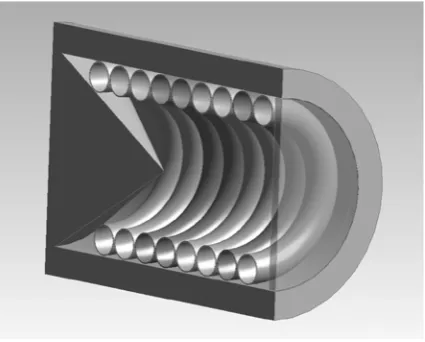
The receiver considered for the purpose of this study is a cylindrical air tube cavity receiver (Qiu, 2015). As shown in Figure3, the receiver is composed of a cylindrical cavity surrounded by insulation. At the bottom of the cavity an optical splitter is used to ensure effective distribution of the solar beam over the inner surface of the receiver and, at the top of the cavity, a quartz glass is presented to minimise the convective heat loss between the receiver and the ambient. The performance of an air tube cavity receiver is strongly influenced by the losses due to natural convection and re-radiation to the surroundings [17] with predominant natural convection losses. The losses caused by the wind forced convection are negligible compared to the natural convection losses. The losses, and thus the efficiency of the receiver can be evaluated using Equations (12)–(15).

Qconv=hconvA(Twall−Tamb). (12)

where the adduction heat transfer coefficienthconvis calculated though the Nusselt number described by Equation (13).

Nuconv=0.88Gr

Tw Tamb

cos(θi)2.47 (13)

where,Gris the Grashoff number,Twis the wall temperature,Tambis the ambient temperature andθi is the inclination angle of the receiver to the vertical direction. Properties of the fluid are calculated at the film temperature, the arithmetic average between the ambient and the wall temperature. The other contribution to losses is due to irradiation phenomena and can be decomposed into two components: the re-irradiation, which is the characteristic of high temperature materials (Equation (14)) and the radiation absorbed by the glass and reflected by the pipe surface (Equation (15)).

Qrad1= Acavεpσb

T_w4−T_amb4 (14)

Qrad2= 1−αpQsun+αgQsun (15)

whereεpis the pipe emissivity,σbis the Stefan-Boltzmann constant,αpandαgare the pipe material and the glass absorptivity, respectively.Qsunis the heat provided by the sun for the given dish diameter and dish optical efficiency. The absorbed heat by the receiver is passed to air, assuming perfect insulation, as given by (Equation (16)).

Qabs=DN I∗Adish∗ηdish−Qconv−Qrad1−Qrad2 = .

mCp(Tin−Tout) =hpAp∆TML. (16)

where:

∆TML=

((Tw−Tin)−(Tw−Tout)) logTw−Tin

Tw−Tout

(17)

(10)

Energies2018,11, 3199 9 of 26

mirror and the deviation of the dish surface from parabolic shape which causes the beam to spread over a wider area than the receiver window.

The receiver considered for the purpose of this study is a cylindrical air tube cavity receiver (Qiu, 2015). As shown in Figure 3, the receiver is composed of a cylindrical cavity surrounded by insulation. At the bottom of the cavity an optical splitter is used to ensure effective distribution of the solar beam over the inner surface of the receiver and, at the top of the cavity, a quartz glass is presented to minimise the convective heat loss between the receiver and the ambient. The performance of an air tube cavity receiver is strongly influenced by the losses due to natural convection and re-radiation to the surroundings [17] with predominant natural convection losses. The losses caused by the wind forced convection are negligible compared to the natural convection losses. The losses, and thus the efficiency of the receiver can be evaluated using Equations (12)–(15).

𝑄𝑄𝑐𝑐𝑜𝑜𝑖𝑖𝑣𝑣=ℎ𝑐𝑐𝑜𝑜𝑖𝑖𝑣𝑣𝐴𝐴(𝑇𝑇𝑤𝑤𝑎𝑎𝑏𝑏𝑏𝑏− 𝑇𝑇𝑎𝑎𝑚𝑚𝑏𝑏) (12)

where the adduction heat transfer coefficient ℎ𝑐𝑐𝑜𝑜𝑖𝑖𝑣𝑣 is calculated though the Nusselt number

described by Equation (13).

𝑁𝑁𝑢𝑢𝑐𝑐𝑜𝑜𝑖𝑖𝑣𝑣= 0.88 𝐽𝐽𝑃𝑃 �_𝑇𝑇𝑇𝑇𝑤𝑤

𝑎𝑎𝑚𝑚𝑏𝑏� 𝑐𝑐𝑐𝑐𝑐𝑐(𝜃𝜃𝑖𝑖)

2.47 ₍₁₃₎

Figure 3. Breakthrough of the adopted cavity receiver.

Where, Gr is the Grashoff number, 𝑇𝑇𝑤𝑤 is the wall temperature, 𝑇𝑇𝑎𝑎𝑚𝑚𝑏𝑏 is the ambient temperature

and 𝜃𝜃𝑖𝑖is the inclination angle of the receiver to the vertical direction. Properties of the fluid are

calculated at the film temperature, the arithmetic average between the ambient and the wall temperature. The other contribution to losses is due to irradiation phenomena and can be decomposed into two components: the re-irradiation, which is the characteristic of high temperature materials (Equation (14)) and the radiation absorbed by the glass and reflected by the pipe surface (Equation (15)).

𝑄𝑄𝑟𝑟𝑎𝑎𝑣𝑣1=𝐴𝐴𝑐𝑐𝑎𝑎𝑣𝑣𝜀𝜀𝑝𝑝𝜎𝜎𝑏𝑏(𝑇𝑇𝑤𝑤4− 𝑇𝑇𝑎𝑎𝑚𝑚𝑏𝑏4 ) (14)

𝑄𝑄𝑟𝑟𝑎𝑎𝑣𝑣2=�1− 𝛼𝛼𝑝𝑝�𝑄𝑄𝑠𝑠𝑜𝑜𝑖𝑖+𝛼𝛼𝑔𝑔𝑄𝑄𝑠𝑠𝑜𝑜𝑖𝑖 (15)

where 𝜀𝜀𝑝𝑝 is the pipe emissivity, 𝜎𝜎𝑏𝑏 is the Stefan-Boltzmann constant, 𝛼𝛼𝑝𝑝 and 𝛼𝛼𝑔𝑔 are the pipe

material and the glass absorptivity, respectively. 𝑄𝑄𝑠𝑠𝑜𝑜𝑖𝑖 is the heat provided by the sun for the given

dish diameter and dish optical efficiency. The absorbed heat by the receiver is passed to air, assuming perfect insulation, as given by (Equation (16)).

𝑄𝑄𝑎𝑎𝑏𝑏𝑠𝑠=𝐷𝐷𝑁𝑁𝐷𝐷 ∗ 𝐴𝐴𝑣𝑣𝑖𝑖𝑠𝑠ℎ∗ 𝜂𝜂𝑣𝑣𝑖𝑖𝑠𝑠ℎ− 𝑄𝑄𝑐𝑐𝑜𝑜𝑖𝑖𝑣𝑣− 𝑄𝑄𝑟𝑟𝑎𝑎𝑣𝑣1− 𝑄𝑄𝑟𝑟𝑎𝑎𝑣𝑣2 = 𝑚𝑚̇𝐶𝐶𝑝𝑝(𝑇𝑇𝑖𝑖𝑖𝑖− 𝑇𝑇𝑜𝑜𝑜𝑜𝑡𝑡) =ℎ𝑝𝑝𝐴𝐴𝑝𝑝𝛥𝛥𝑇𝑇𝑀𝑀𝑀𝑀 (16)

where:

𝛥𝛥𝑇𝑇𝑀𝑀𝑀𝑀=�(𝑇𝑇𝑤𝑤− 𝑇𝑇𝑖𝑖𝑖𝑖)−(𝑇𝑇𝑤𝑤− 𝑇𝑇𝑜𝑜𝑜𝑜𝑡𝑡)�

𝑙𝑙𝑐𝑐𝑙𝑙 � 𝑇𝑇𝑤𝑤− 𝑇𝑇𝑖𝑖𝑖𝑖

𝑇𝑇𝑤𝑤− 𝑇𝑇𝑜𝑜𝑜𝑜𝑡𝑡�

[image:10.595.192.405.126.297.2]

(17) Figure 3.Breakthrough of the adopted cavity receiver.

The heat transfer and the pressure losses within the receiver pipe are evaluated considering a helically coiled tube. Many validated correlations to describe the heat transfer characteristics of a helicoidally coiled pipe are available in the literature. The model adopted in this study is the one proposed by Xin and Ebadian [18].

2.2. Cost Analysis

A detailed techno-economic analysis was carried out to evaluate the cost and the levelised cost of electricity of the plant in different arrangements. The analysis is based on the components’ models and a series of cost functions to evaluate individual cost of each components, and other elements of cost of the system such as installation and maintenance.

Unlike large-scale gas turbines, only a few cost evaluation studies are available in literature for microturbines. For this study, the approach used by Galanti [19] has been used and the cost functions for the different components are described by the following equations where all the costs are given in euros.

Ccompr.=55.8∗ln(PRc)∗

.

m 0.942−ηpc

(18)

Cturb.=376.1∗ln(PRt)∗

_m.

0.903−ηpt

(19)

Crecup.=9fm 625.1 . m

pin∆p

100 −0.5

∗

ε

1−ε

!

(20)

Cgen.=18.7P0.95 (21)

wherePRcandPRtare the compressor and turbine pressure ratios,pinis the inlet pressure expressed in bar,∆pis the recuperator percentage pressure loss,m. is the mass flow rate in kg/s,εis the recuperator

effectiveness andPis the net power output in kW. The cost of the generator also includes the cost of power electronics and has been evaluated using Equation (21). The receiver cost function was interpolated from a study conducted by Pioneer Engineering [20] for a pressurised air solar receiver, adaptable for a solar dish and microturbine system. The study considered direct labour costs, direct material costs and manufacturing costs. Results from this study were interpolated and Equation (22) was obtained which expresses the cost of the receiver as a function of absorbed heat.

(11)

In this equation,QRecis the receiver input heat expressed in watts. The dish cost by far has the biggest contribution to the plant cost [7] and it needs careful consideration for adequate prediction of the cost. In this study, the dish cost was evaluated using a regression model as described by Equation (23) based on a study conducted by [21]. The study evaluated the specific prices of collectors in the range from 67 m2to 230 m2for different production volumes. According to [7] the exponent nDishdoes not vary significantly from unity for a wide range of dish diameters, and, for this reason, a linear dependency of the dish cost on the area was considered.

CDish=260∗An_Dishdish (23)

whereADishis the dish surface area in [m2]. The overall cost can be then calculated using Equation (24).

CTOT=CMGT+CRec+CDish+Cinst (24)

In the previous equation,Cinstis the installation cost, which includes the cost of installation and other costs not related directly to components. On the base of the findings of a study conducted by Gavagnin et al. [7], this has been approximated as 17% of the total components’ costs. Using the Chemical Engineering Plant Cost Index (CEPCI) each calculated cost was discounted to update the costs at the current year as described in (Equation (25)).

Cj=

Cref∗ CEPCIj

(CEPCIref)

(25)

whereCjis the cost at year j, CEPCIjis the Chemical Engineering Plant Cost Index for year, j,Crefis a known cost of the components for a particular year and CEPCIrefis taken for the same reference year. The levelised cost of electricity therefore can be calculated using Equation (26).

LCOE= αCTOT+CO&M

E (26)

α= i∗(1+i)

n

(1+i)n−1 (27)

The capital recovery factorαhas been evaluated considering typical values ofi= 0.07 for the

actual interest rate andn= 25 years for the lifetime of the plant. Operation and maintenance costs have been estimated to be 5% of the total cost as suggested by [22]. Costs of operation and maintenance has been considered as 5% of total costs, which includes capital and installation costs. Scale economy related to different production rates were not considered in this study.

2.3. Model Validation

In this section the model validation is presented. Given the lack of experimental data regarding solar dish-MGT power plant, the validation has been performed for each component. One or more validation case studies for similar designs to those investigated in this paper were considered for each component and results output from the present model have been compared with experimental data available in literature. Data about the models validation can be found in the supplementary materials provided by the authors.

2.3.1. Compressor Off-Design Model Validation

(12)

Energies2018,11, 3199 11 of 26

error of 2.5% for the efficiency and 3% for the pressure ratio. Moreover, the curves demonstrate comparable behaviour and the error is located only in short sections of the curves. The same observations are valid for the Eckardt impeller A. In this case the model shows a maximum relative error of 4% for the efficiency and 4.3% for the pressure ratio. Despite the higher maximum relative error, the overall accuracy of the model is higher when compared with the Eckardt impeller A, especially regarding efficiency. On the other hand, the pressure ratio shows a more accentuated slope of the curve when getting close to the choking limit. Nevertheless, the accuracy of the model was considered acceptable for the purpose of this study.

For the case of KIMM compressor geometry, the efficiency chart was not available and the comparison has been performed only on the pressure ratio. Results show better agreement with the experimental results when compared to the other two compressor geometries showing a maximum relative error of 1.5%. This demonstrates the suitability of the present model for smaller size compressors.

(a) Eckardt Impeller O (b) Eckardt Impeller A (c) KIMM Impeller

Figure 4. Impeller geometries considered for the validation (not in scale) [23]. (a) Eckardt impeller O. (b) Eckardt impeller A. (c) KIMM impeller.

(a) (b)

Figure 5. Compressor validation: characteristic maps for Eckardt impeller O. (a) Total to static isentropic efficiency vs mass flow rate; (b) pressure ratio vs mass flow rate.

(a) (b)

0.8 0.82 0.84 0.86 0.88 0.9

1.5 3.5 5.5 7.5

ηs,TS

Mass Flow [kg/s]

1 1.4 1.8 2.2 2.6 3

1.5 3.5 5.5 7.5

PR

0.75 0.8 0.85 0.9 0.95

1.5 3.5 5.5 7.5

ηs,TS

1 1.5 2 2.5

0 2 4 6 8

PR

[image:12.595.91.510.278.426.2]

Figure 4.Impeller geometries considered for the validation (not in scale) [23]. (a) Eckardt impeller O. (b) Eckardt impeller A. (c) KIMM impeller.

(a) (b)

0.8 0.82 0.84 0.86 0.88 0.9

1.5 3.5 5.5 7.5

ηs,TS

1 1.4 1.8 2.2 2.6 3

1.5 3.5 5.5 7.5

PR

0.75 0.8 0.85 0.9 0.95

1.5 3.5 5.5 7.5

ηs,TS

1 1.5 2 2.5

0 2 4 6 8

PR

[image:12.595.90.509.463.681.2]

(13)

Energies2018,11, 3199 12 of 26

(a) (b)

0.8 0.82 0.84 0.86 0.88 0.9

1.5 3.5 5.5 7.5

ηs,TS

1 1.4 1.8 2.2 2.6 3

1.5 3.5 5.5 7.5

PR

0.75 0.8 0.85 0.9 0.95

1.5 3.5 5.5 7.5

ηs,TS

1 1.5 2 2.5

0 2 4 6 8

PR

[image:13.595.82.505.84.306.2] [image:13.595.81.502.340.558.2]

Figure 6.Compressor validation: characteristic maps for Eckardt impeller A. (a) Total to static isentropic efficiency vs mass flow rate; (b) pressure ratio vs mass flow rate.

Figure 6. Compressor validation: characteristic maps for Eckardt impeller A. (a) Total to static isentropic efficiency vs mass flow rate; (b) pressure ratio vs mass flow rate.

Figure 7. Compressor validation: characteristic maps for KIMM impeller.

2.3.2. Recuperator Off-Design Model Validation

The model for the recuperator has been validated against available experimental data for a range of fin geometries as proposed by [24]. The fin geometries and arrangements used for the validation, namely, 1/10-27.03 and 1/8-16.00(D) fin geometries, are presented in Figure 8 and more details of the geometry are given in [24].

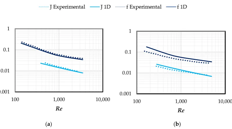
Figure 9 shows the modelling results of the Colburn factor (J) and friction factor (f) for both 1/10-27.03 and 1/8-16.00(D) fin geometries. The modelling for the first geometry presents a maximum relative error of 3% for both Colburn factor and friction factor. Nevertheless, there is some inaccuracy in the results of the second fin geometry, with a maximum relative error around 18% for the Colburn number and 6% for the friction factor. Given the higher accuracy of the model in predicting the performance of the 1/10-27.03 fin geometry, this layout will be adopted by the model for the recuperator design.

(a) (b)

Figure 7.Compressor validation: characteristic maps for KIMM impeller.

The model for the recuperator has been validated against available experimental data for a range of fin geometries as proposed by [24]. The fin geometries and arrangements used for the validation, namely, 1/10-27.03 and 1/8-16.00(D) fin geometries, are presented in Figure8and more details of the geometry are given in [24].

(14)

Energies2018,11, 3199 13 of 26

Figure 6. Compressor validation: characteristic maps for Eckardt impeller A. (a) Total to static isentropic efficiency vs mass flow rate; (b) pressure ratio vs mass flow rate.

Figure 7. Compressor validation: characteristic maps for KIMM impeller.

The model for the recuperator has been validated against available experimental data for a range of fin geometries as proposed by [24]. The fin geometries and arrangements used for the validation, namely, 1/10-27.03 and 1/8-16.00(D) fin geometries, are presented in Figure 8 and more details of the geometry are given in [24].

Figure 9 shows the modelling results of the Colburn factor (J) and friction factor (f) for both 1/10-27.03 and 1/8-16.00(D) fin geometries. The modelling for the first geometry presents a maximum relative error of 3% for both Colburn factor and friction factor. Nevertheless, there is some inaccuracy in the results of the second fin geometry, with a maximum relative error around 18% for the Colburn number and 6% for the friction factor. Given the higher accuracy of the model in predicting the performance of the 1/10-27.03 fin geometry, this layout will be adopted by the model for the recuperator design.

[image:14.595.83.486.89.234.2]

(a) (b)

Figure 8. Fin geometries and arrangement considered for the recuperator model validation [24]. (a) 1/10-27.03; (b) 1/8-16.00(D).

Figure 8. Fin geometries and arrangement considered for the recuperator model validation [24]. (a) 1/10-27.03; (b) 1/8-16.00(D).

(a) (b)

Figure 9. Comparison between experimental and analytical data. Colburn factor (cyan) and friction factor (blue). (a) Fin geometry 1/10-27.03. (b) Fin geometry 1/8-16.00(D).

2.3.3. Receiver off-Design Model Validation

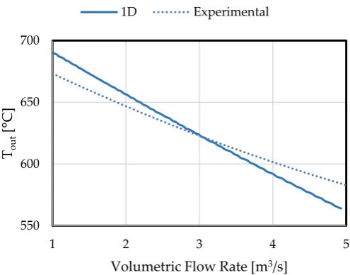
The receiver model was validated by comparing the results obtained from the one-dimensional model with experimental results available in literature [25]. The receiver consists of 15-turn helically coiled copper tube with inner diameter of 12 mm and thickness of 1 mm. The inner diameter and height of the cavity are 140 mm and 200 mm, respectively.

Results shown in Figure 10 demonstrate good agreement concerning outlet temperature for a wide range of operating points with a maximum relative error below 2.5%,which is considered adequate for the purpose of this study.

Figure 10. Results from receiver validation. 550

600 650 700

1 2 3 4 5

Tout

[

°

C]

Volumetric Flow Rate [m3_/s]

1D Experimental

0.001 0.01 0.1 1

100 1,000 10,000

Re

0.001 0.01 0.1 1

100 1,000 10,000

[image:14.595.100.499.271.493.2]

Re

Figure 9.Comparison between experimental and analytical data. Colburn factor (cyan) and friction factor (blue). (a) Fin geometry 1/10-27.03. (b) Fin geometry 1/8-16.00(D).

(15)

Energies2018,11, 3199 14 of 26 Figure 8. Fin geometries and arrangement considered for the recuperator model validation [24]. (a) 1/10-27.03; (b) 1/8-16.00(D).

(a) (b)

Figure 9. Comparison between experimental and analytical data. Colburn factor (cyan) and friction factor (blue). (a) Fin geometry 1/10-27.03. (b) Fin geometry 1/8-16.00(D).

[image:15.595.174.422.87.281.2]

Results shown in Figure 10 demonstrate good agreement concerning outlet temperature for a wide range of operating points with a maximum relative error below 2.5%, which is considered adequate for the purpose of this study.

Figure 10. Results from receiver validation. 550

600 650 700

1 2 3 4 5

Tout

[

°

C]

Volumetric Flow Rate [m3_/s]

1D Experimental

0.001 0.01 0.1 1

100 1,000 10,000

Re

0.001 0.01 0.1 1

100 1,000 10,000

Re

Figure 10.Results from receiver validation.

2.3.4. Turbine Off-Design Model Validation

[image:15.595.141.454.398.528.2]

The turbine model was validated against experimental data available in literature for a similar design [26] in terms of size and expansion ratio. Table1presents the main geometrical parameters of the turbine adopted for validation.

Table 1.Turbine geometrical specifications.

Rotor Inlet Tip Diameter 99.1 mm Rotor inlet tip width 10.2 mm Rotor inlet axial clearance, back-plate side 0.25 mm Rotor inlet axial clearance, shroud side 0.4 mm

Rotor inlet blade angle 0◦

Rotor blade number 11

Rotor exducer tip diameter 79.0 mm Rotor exducer hub diameter 30.0 mm Rotor exducer blade angle 50.1◦ Rotor exducer blade thickness 1.6 mm

Rotor exit radial clearance 0.4 mm

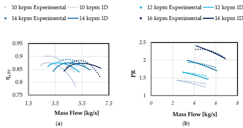
Results of turbine model validation demonstrate good accuracy for a wide range of operational conditions, which also covers the actual operating condition of turbines of interest for this study (Figure11). The model reproduces satisfactorily the behavior of the turbine, especially near choking condition, while for a given rotational speed, it seems to lose its accuracy towards lower mass flow rates. Nevertheless, the maximum relative error is low, apart from in a few working conditions where it reaches 13.1%. Although the coefficient of determination, calculated using Equation (28), decreases with the rotational speed it stays above 0.994. This ensures sufficient accuracy when predicting the corrected mass flow rate and the efficiency as functions of rotational speed and pressure ratio. Moreover, the inaccuracy of the model is associated within working points not representing typical working conditions and may not affect the accuracy of the cycle simulation.

R2=1−∑(yi−yˆi)

2

∑(yi−yi)2

(28)

(16)

Energies2018,11, 3199 15 of 26

2.3.4. Turbine Off-Design Model Validation

The turbine model was validated against experimental data available in literature for a similar design [26] in terms of size and expansion ratio. Table 1 presents the main geometrical parameters of the turbine adopted for validation.

Table 1. Turbine geometrical specifications.

Rotor Inlet Tip Diameter 99.1 mm

Rotor inlet tip width 10.2 mm

Rotor inlet axial clearance, back-plate side 0.25 mm Rotor inlet axial clearance, shroud side 0.4 mm

Rotor inlet blade angle 0°

Rotor blade number 11

Rotor exducer tip diameter 79.0 mm

Rotor exducer hub diameter 30.0 mm

Rotor exducer blade angle 50.1°

Rotor exducer blade thickness 1.6 mm

Rotor exit radial clearance 0.4 mm

[image:16.595.121.471.91.300.2]

Results of turbine model validation demonstrate good accuracy for a wide range of operational conditions, which also covers the actual operating condition of turbines of interest for this study (Figure 11). The model reproduces satisfactorily the behavior of the turbine, especially near choking condition, while for a given rotational speed, it seems to lose its accuracy towards lower mass flow rates. Nevertheless, the maximum relative error is low, apart from in a few working conditions where it reaches 13.1%. Although the coefficient of determination, calculated using Equation (28), decreases with the rotational speed it stays above 0.994. This ensures sufficient accuracy when predicting the corrected mass flow rate and the efficiency as functions of rotational speed and pressure ratio. Moreover, the inaccuracy of the model is associated within working points not representing typical working conditions and may not affect the accuracy of the cycle simulation.

𝑅𝑅2_{= 1}₋∑(𝑦𝑦𝑖𝑖− 𝑦𝑦�)𝚤𝚤 2

∑(𝑦𝑦𝑖𝑖− 𝑦𝑦�)𝚤𝚤 2 (28)

In Equation (28), 𝑦𝑦𝑖𝑖 is the predicted value, 𝑦𝑦�𝚤𝚤 is the observed value and 𝑦𝑦�𝚤𝚤 is the mean value of

the observed data.

(a) (b)

Figure 11. Results from turbine validation. (a) Corrected flow rate vs pressure ratio; (b) total to static isentropic efficiency vs pressure ratio.

0.12 0.14 0.16 0.18 0.2 0.22

1 1.5 2 2.5 3

μ

[k

g/s

]

PR

0.6 0.65 0.7 0.75 0.8 0.85

1 1.5 2 2.5 3

ηs,TS

PR

Figure 11.Results from turbine validation. (a) Corrected flow rate vs pressure ratio; (b) total to static isentropic efficiency vs pressure ratio.

3. Results

In this section a case study for a 7-kWeMGT is discussed and the techno-economic performance of the plant is evaluated using the presented models. For verification of the components’ matching a model developed in the commercial software IPSEpro, was used. The benchmark results for a pure-solar MGT-based CSP power plant are presented below. Finally, a plant-size optimisation has been performed to identify feasible economic solutions for a given set of conditions such as local solar irradiation pattern.

3.1. Case Study

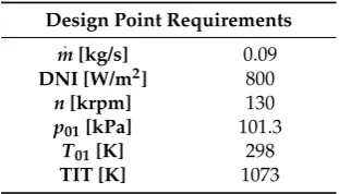
[image:16.595.220.376.570.659.2]

In this section a case study considering a 7-kWe pure-solar plant powered by microturbine is presented. The plant consists of a compressor, recuperator, solar receiver, turbine and a high-speed generator to convert the available mechanical energy to electricity. Preliminary design characteristics have been chosen based on the findings of the OMSoP project [6] and a previous study conducted by the authors [27]. Table2reports the preliminary design characteristics of the plant.

Table 2.Main design requirements.

Design Point Requirements .

m[kg/s] 0.09

DNI [W/m2] 800

n[krpm] 130

p01[kPa] 101.3

T01[K] 298

TIT [K] 1073

(17)

Energies2018,11, 3199 16 of 26 3. Results

In this section a case study for a 7-kWe MGT is discussed and the techno-economic performance of the plant is evaluated using the presented models. For verification of the components’ matching a model developed in the commercial software IPSEpro, was used. The benchmark results for a pure-solar MGT-based CSP power plant are presented below. Finally, a plant-size optimisation has been performed to identify feasible economic solutions for a given set of conditions such as local solar irradiation pattern.

3.1. Case Study

In this section a case study considering a 7-kWe pure-solar plant powered by microturbine is presented. The plant consists of a compressor, recuperator, solar receiver, turbine and a high-speed generator to convert the available mechanical energy to electricity. Preliminary design characteristics have been chosen based on the findings of the OMSoP project [6] and a previous study conducted by the authors [27]. Table 2 reports the preliminary design characteristics of the plant.

Table 2. Main design requirements.

Design Point Requirements

𝒎𝒎̇[kg/s] 0.09

DNI [W/m2_] ₈₀₀

n [krpm] 130

p01 [kPa] 101.3

T01 [K] 298

TIT [K] 1073

The study has been performed considering data available in literature for solar irradiation in Rome for the period between 2004 and 2005. Figure 12 shows the DNI frequency diagram and the moving average of the DNI for a constant variation of 100 W/m2_{in the DNI. As can be seen in this} figure, the highest average frequency levels are for the DNI are around the value of 800 W/m2_{. For} this reason, this value has been chosen as design DNI while DNIs lower than 300 W/m2 have not been investigated due to negligible power that can be produced in such solar irradiation level.

Figure 12. DNI frequencies in Rome for the period between 2004 and 2005 and the moving average of DNI (red line).

0 2 4 6 8 10 12 14

200 300 400 500 600 700 800 900

Fre

que

nc

y [

h/

y]

[image:17.595.121.478.91.249.2]

DNI [W/m2]

Figure 12.DNI frequencies in Rome for the period between 2004 and 2005 and the moving average of DNI (red line).

3.2. Design Results

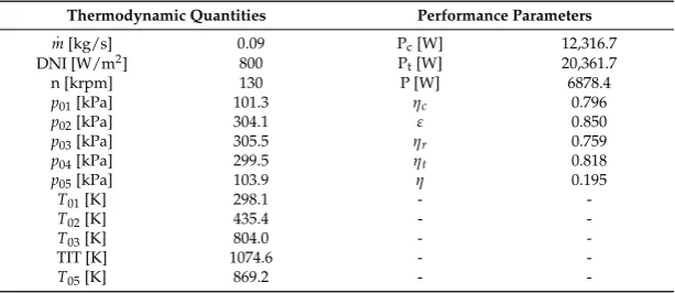
The results from the design procedure are presented in Table3based on the design requirements presented in Table2and the chosen DNI. The net power output has been evaluated considering mechanical and electrical efficiencies of 85% and 90%, respectively.

Using the models discussed previously, each component of the system was designed based on the performance parameters given in Table3. The compressor is composed of an impeller with 12 blades and a vaneless diffuser of 60 mm radius. The impeller has a tip exit radius of 36 mm and width of 1.5 mm; the isentropic efficiency of the compressor is 0.80. The fin geometry 1/10-27.03 has been adopted for the recuperator and it has an overall heat transfer area of about 17 m2and a heat transfer to volume ratio of around 2900 m−1. Its effectiveness was set to 0.85 and the heat transfer coefficient was evaluated at 163 W/m2K and 119 W/m2K on the hot and cold sides, respectively. The pressure drop is estimated to be 1% on the hot side and 3% on the cold side. The receiver is characterised by a cavity diameter of 19 cm and length of 33.6 cm. The overall length of the pipe, which has a diameter of 4 cm, is 3.748 m, and is formed of a helical coiled pipe with 8 turns.The efficiency of the receiver is 0.76 while the overall pressure loss is around 3%. Based on the receiver performance, the dish aperture diameter required to produce the desired electrical power of 7 kWe is 8.37 m, assuming dish optical efficiency of 0.8. The turbine impeller, with isentropic efficiency of 0.799, consists of 11 blades with an inlet radius of 38.5 mm, exit hub radius of 14.9 mm and exit tip radius of 28.6 mm. AppendixA

[image:17.595.145.452.582.715.2]

summarises the design parameters of the plant components.

Table 3.The design parameters for the 7-kWe plant.

Thermodynamic Quantities Performance Parameters

.

m[kg/s] 0.09 Pc[W] 12,316.7

DNI [W/m2_] ₈₀₀ _P

t[W] 20,361.7

n [krpm] 130 P [W] 6878.4

p01[kPa] 101.3 ηc 0.796

p02[kPa] 304.1 ε 0.850

p03[kPa] 305.5 ηr 0.759

p04[kPa] 299.5 ηt 0.818

p05[kPa] 103.9 η 0.195

T01[K] 298.1 -

-T02[K] 435.4 -

-T03[K] 804.0 -

-TIT [K] 1074.6 -

-T05[K] 869.2 -

-3.3. IPSEpro Simulation Set-Up

(18)

Energies2018,11, 3199 17 of 26

The layout of the process units of the model is shown in Figure1. Characteristics maps for the turbomachinery and recuperator have been generated based on the validated models of components as discussed in the preceding section and are implemented in the IPSEpro model for off-design calculations. Input parameters are rotational speed, DNI and ambient conditions, i.e., air relative humidity, ambient pressure and ambient temperature. The TIT is considered as constraint with maximum allowable limit of 1073±1 K. When the limit of TIT is reached, the rotational speed, thus the air mass flow rate, and turbine outlet temperature are regulated to avoid exceeding the limit. The model outputs are pressure, temperature, mass flow rate and enthalpy downstream and upstream of the components, by which performance indicators such as power and electrical efficiency are calculated. The physical properties of gas components are calculated with polynomials derived from the JANAF (Joint Army Navy Air Force) Thermodynamic Tables [28]. In IPSEpro, all calculations were performed assuming that the gas components being ideal gases.

3.4. Off-Design Results

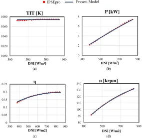
For a typical pure-solar application, the MGT operates at a constant TIT (at the highest allowable level) to maximise the overall efficiency of the plant. It should be noted that here, the TIT has been limited due to material limitation of the receiver rather than the turbine material. In case of OMSoP plant this limit was estimated to 1073 K. To achieve a constant TIT, it is necessary to operate at variable mass flow rate and consequently variable rotational speed. For lower DNIs it would not be possible to achieve the highest allowable TIT, which means that the MGT will operate at lower efficiency. Moreover, the power output for these operating points is relatively low, as is their occurrence frequency as shown in Figure13. As such, a minimum output power of the plant was fixed to 2000 W and points with lower power output were not considered. It should be emphasised that considering any power below this level would neither change the annual produced electricity significantly nor the levelised cost of electricity.

Energies 2018, 11, x FOR PEER REVIEW 17 of 27

3.4. Off-Design Results

For a typical pure-solar application, the MGT operates at a constant TIT (at the highest allowable level) to maximise the overall efficiency of the plant. It should be noted that here, the TIT has been limited due to material limitation of the receiver rather than the turbine material. In case of OMSoP plant this limit was estimated to 1073 K. To achieve a constant TIT, it is necessary to operate at variable mass flow rate and consequently variable rotational speed. For lower DNIs it would not be possible to achieve the highest allowable TIT, which means that the MGT will operate at lower efficiency. Moreover, the power output for these operating points is relatively low, as is their occurrence frequency as shown in Figure 13. As such, a minimum output power of the plant was fixed to 2000 W and points with lower power output were not considered. It should be emphasised that considering any power below this level would neither change the annual produced electricity significantly nor the levelised cost of electricity.

(a) (b)

[image:18.595.154.440.442.719.2]

(c) (d)

Figure 13. Plant off-design performance charts under variable DNI. (a) TIT; (b) output power; (c) efficiency; (d) rotational speed.

The results of the present model have been compared with the results from IPSEpro where the same component characteristic maps and operational strategy were considered. This comparison was aimed to verify the component matching procedure adopted for the present model. The results in Figure 13 demonstrate good accuracy for the whole range of operation. The discrepancy in the results is due to the setup in IPSEpro where the TIT is limited not to a single value, 1073 K in this case, but

1000 1020 1040 1060 1080

300 500 700 900

DNI [W/m2_]

TIT [K]

0 2 4 6 8

300 500 700 900

DNI [W/m2_]

P [kW]

0 0.05 0.1 0.15 0.2 0.25

300 400 500 600 700 800 900

DNI [W/m2]

η