THE SPITZER MICROLENSING PROGRAM AS A PROBE FOR GLOBULAR CLUSTER PLANETS:
ANALYSIS OF OGLE-2015-BLG-0448
Radosław Poleski1,2, Wei Zhu1, Grant W. Christie3, Andrzej Udalski2, Andrew Gould1,4,5, Etienne Bachelet6, Jesper Skottfelt7,8, Sebastiano Calchi Novati9,10,11,
M. K. SzymaŃski2, I. SoszyŃski2, G. PietrzyŃski2,12,Ł. Wyrzykowski2, K. Ulaczyk2,13, P. Pietrukowicz2, Szymon Kozłowski2, J. Skowron2, P. MrÓz2, M. Pawlak2
(OGLE group),
C. Beichman9, G. Bryden14, S. Carey14, M. Fausnaugh1, B. S. Gaudi1, C. B. Henderson14,52, R. W. Pogge1, Y. Shvartzvald14,52, B. Wibking1, J. C. Yee15,53
(Spitzer team),
T. G. Beatty16, J. D. Eastman15, J. Drummond17, M. Friedmann18, M. Henderson19, J. A. Johnson15, S. Kaspi8, D. Maoz18, J. McCormick20, N. McCrady19, T. Natusch3,21, H. Ngan3, I. Porritt22, H. M. Relles15, D. H. Sliski52, T.-G. Tan24,
R. A. Wittenmyer25,26,27, J. T. Wright16 (μFUN group),
R. A. Street6, Y. Tsapras28, D. M. Bramich29, K. Horne30, C. Snodgrass31, I. A. Steele32, J. Menzies33, R. Figuera Jaimes30,34, J. Wambsganss28, R. Schmidt28, A. Cassan35, C. Ranc35, S. Mao36
(RoboNet project), and
V. Bozza10,37, M. Dominik30,51, M. P. G. Hundertmark8, U. G. Jørgensen8, M. I. Andersen38, M. J. Burgdorf39, S. Ciceri40, G. D’Ago10,11,37, D. F. Evans41, S.-H. Gu42, T. C. Hinse43, N. Kains44, E. Kerins44, H. Korhonen45,8, M. Kuffmeier8, L. Mancini40, A. Popovas8, M. Rabus46, S. Rahvar47, R. T. Rasmussen48, G. Scarpetta10,11, J. Southworth41, J. Surdej49,
E. Unda-Sanzana50, P. Verma11, C. von Essen48, Y.-B. Wang42, and O. Wertz49 (MiNDSTEp group)
1
Department of Astronomy, Ohio State University, 140 West 18th Avenue, Columbus, OH 43210, USA;[email protected]
2
Warsaw University Observatory, Al. Ujazdowskie 4, 00-478 Warszawa, Poland 3
Auckland Observatory, Auckland, New Zealand 4
Max-Planck-Institute for Astronomy, Königstuhl 17, D-69117 Heidelberg, Germany 5
Korea Astronomy and Space Science Institute, Daejon 305-348, Republic of Korea 6
Las Cumbres Observatory Global Telescope Network, 6740 Cortona Drive, Suite 102, Goleta, CA 93117, USA 7
Centre for Electronic Imaging, Department of Physical Sciences, The Open University, Milton Keynes MK7 6AA, UK 8
Niels Bohr Institute & Centre for Star and Planet Formation, University of Copenhagen, Øster Voldgade 5, DK-1350—Copenhagen K, Denmark 9
NASA Exoplanet Science Institute, MS 100-22, California Institute of Technology, Pasadena, CA 91125, USA 10Dipartimento di Fisica“E.R. Caianiello,” Università di Salerno, Via Giovanni Paolo II 132, I-84084, Fisciano, Italy 11
Istituto Internazionale per gli Alti Studi Scientifici(IIASS), Via G. Pellegrino 19, I-84019 Vietri sul Mare(SA), Italy 12
Universidad de Concepción, Departamento de Astronomia, Casilla 160C, Concepción, Chile 13
Department of Physics, University of Warwick, Coventry CV4 7AL, UK 14
Jet Propulsion Laboratory, California Institute of Technology, 4800 Oak Grove Drive, Pasadena, CA 91109, USA 15
Harvard-Smithsonian Center for Astrophysics, 60 Garden Street, Cambridge, MA 02138, USA 16
Department of Astronomy and Astrophysics and Center for Exoplanets and Habitable Worlds, The Pennsylvania State University, University Park, PA 16802, USA 17
Possum Observatory, Patutahi, New Zealand 18
School of Physics and Astronomy, Tel-Aviv University, Tel-Aviv 69978, Israel 19
Department of Physics and Astronomy, University of Montana, 32 Campus Drive, No. 1080, Missoula, MT 59812, USA 20
Farm Cove Observatory, Centre for Backyard Astrophysics, Pakuranga, Auckland, New Zealand 21
AUT University, Auckland, New Zealand 22
Turitea Observatory, Palmerston North, New Zealand 23
The University of Pennsylvania, Department of Physics and Astronomy, Philadelphia, PA, 19104, USA 24
Perth Exoplanet Survey Telescope, Perth, Australia 25
School of Physics and Australian Centre for Astrobiology, UNSW Australia, Sydney, NSW 2052, Australia 26
Australian Centre for Astrobiology, University of New South Wales, Sydney 2052, Australia 27
Computational Engineering and Science Research Centre, University of Southern Queensland, Toowoomba, Queensland 4350, Australia 28
Astronomisches Rechen-Institut, Zentrum für Astronomie der Universität Heidelberg(ZAH), D-69120 Heidelberg, Germany 29
Qatar Environment and Energy Research Institute(QEERI), HBKU, Qatar Foundation, Doha, Qatar 30
SUPA, School of Physics & Astronomy, University of St Andrews, North Haugh, St Andrews KY16 9SS, UK 31
Planetary and Space Sciences, Department of Physical Sciences, The Open University, Milton Keynes, MK7 6AA, UK 32
Astrophysics Research Institute, Liverpool John Moores University, Liverpool CH41 1LD, UK 33
South African Astronomical Observatory, P.O. Box 9, Observatory 7935, South Africa 34
European Southern Observatory, Karl-Schwarzschild-Str. 2, D-85748 Garching bei München, Germany 35
Sorbonne Universités, UPMC Univ Paris 6 et CNRS, UMR 7095, Institut d’Astrophysique de Paris, 98 bis bd Arago, F-75014 Paris, France 36
National Astronomical Observatories, Chinese Academy of Sciences, 100012 Beijing, China 37
Istituto Nazionale di Fisica Nucleare, Sezione di Napoli, Napoli, Italy 38
Niels Bohr Institute, University of Copenhagen, Juliane Maries Vej 30, DK-2100 København Ø, Denmark 39
Meteorologisches Institut, Universität Hamburg, Bundesstraße 55, D-20146 Hamburg, Germany 40
Max Planck Institute for Astronomy, Königstuhl 17, D-69117 Heidelberg, Germany 41
Astrophysics Group, Keele University, Staffordshire, ST5 5BG, UK 42
43
Korea Astronomy & Space Science Institute, 776 Daedukdae-ro, Yuseong-gu, 305-348 Daejeon, Korea
44Jodrell Bank Centre for Astrophysics, School of Physics and Astronomy, University of Manchester, Oxford Road, Manchester M13 9PL, UK 45
Finnish Centre for Astronomy with ESO(FINCA), Väisäläntie 20, FI-21500 Piikkiö, Finland 46
Instituto de Astrofísica, Facultad de Física, Pontificia Universidad Católica de Chile, Av. Vicuña Mackenna 4860, 7820436 Macul, Santiago, Chile 47
Department of Physics, Sharif University of Technology, P.O. Box 11155-9161 Tehran, Iran 48
Stellar Astrophysics Centre, Department of Physics and Astronomy, Aarhus University, Ny Munkegade 120, DK-8000 Aarhus C, Denmark 49
Institut d’Astrophysique et de Géophysique, Allée du 6 Août 17, Sart Tilman, Bât. B5c, B-4000 Liège, Belgium 50
Unidad de Astronomía, Fac. de Ciencias Básicas, Universidad de Antofagasta, Avda. U. de Antofagasta 02800, Antofagasta, Chile Received 2015 December 23; accepted 2016 March 20; published 2016 May 23
ABSTRACT
The microlensing event OGLE-2015-BLG-0448 was observed by Spitzer and lay within the tidal radius of the globular cluster NGC 6558. The event had moderate magnification and was intensively observed, hence it had the potential to probe the distribution of planets in globular clusters. We measure the proper motion of NGC 6558
(m N E, = +0.360.10,+1.420.10 mas yr
-cl( ) ( ) 1) as well as the source and show that the lens is not a cluster member. Even though this particular event does not probe the distribution of planets in globular clusters, other potential cluster lens events can be verified using our methodology. Additionally, we find that microlens parallax measured using Optical Gravitational Lens Experiment (OGLE)photometry is consistent with the value found based on the light curve displacement between the Earth andSpitzer.
Key words:globular clusters: individual (NGC6558)–gravitational lensing: micro– planets and satellites: detection– proper motions
1. INTRODUCTION
The Spitzer gravitational microlensing project has as its principal aim the determination of the Galactic distribution of planets(Gould et al.2014). This primarily means usingSpitzer to measure“microlens parallaxes”pE and thereby estimate the distances of the individual lenses. By comparing this overall distance distribution to the one restricted to events showing planetary signatures, one can determine whether planets are more common in, for example, the Galactic disk or the bulge
(Calchi Novati et al.2015a; Yee et al.2015). Among the 170 microlensing events observed during the 2015 campaign
(Calchi Novati et al. 2015b), one event showed potential for a very different probe of the“Galactic distribution of planets,” namely, of the frequency of planets in globular clusters
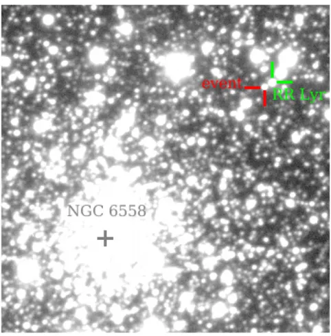
(relative to disk or bulge stars). The event OGLE-2015-BLG-0448 lay projected against the globular cluster NGC 6558
(Figure1), and therefore the lens was potentially a member of this cluster. The lens mass is measured if one knows the relative lens-source parallax and the angular size of the Einstein ring radius (Refsdal 1964). In the case of a globular cluster lens, one can, in principle, derive the lens mass based on the Einstein timescale measurement alone (knowing the cluster distance and proper motion from the literature; Paczyński 1994). In reality, significant uncertainties are introduced by the dispersion of bulge source proper motions that is comparable to the cluster proper motion.
Here we present a new method to determine whether the lens from a microlensing event seen projected against a cluster is in fact a cluster member, employing observations of the Spitzer spacecraft as a“microlensing parallax satellite.”The method is to compare the direction of the heliocentric projected velocity
v˜helwith that of the proper motion of the cluster relative to the microlensed sourcemcl,s. As is well known,v˜helcan be subject to a four-fold degeneracy in direction (Refsdal 1966; Gould 1994), but within those degenerate solutions can be very precisely measured by a parallax satellite (Calchi Novati
et al.2015a). Therefore, ifmcl,scan also be measured precisely, the hypothesis of the cluster lens can be tested with high precision.
The analyzed event was unusually sensitive to planets, independent of the possibility that the lens might be a cluster member. First, the source star is a low-luminosity giant, meaning that photometry from both the ground and space was unusually precise. Second, it reached magnificationAmax »13
as seen from both the Earth and Spitzer. Such moderate magnification events are substantially more sensitive to planets than typical events (Mao & Paczyński 1991; Gould & Loeb1992). The combination of these factors led to relatively intensive monitoring from the ground and exceptionally intensive monitoring from Spitzer, which further increased the event’s planet sensitivity. We show that Spitzer residuals from point-lens models can befitted with a Saturn-mass ratio double-lens model. We do not claim planet detection because Spitzer photometry of neighboring constant stars shows systematic trends that could mimic the planetary signal if superimposed on a purely point-lens (Paczyński 1986) light curve. The only known planet in a globular cluster is in a system with a white dwarf and pulsar (Richer et al. 2003; Nascimbeni et al.2012).
The light curve of OGLE-2015-BLG-0448 is analyzed here for two different purposes: to measure the microlens parallax and to estimate the planet sensitivity. The available ground-based data are survey observations by the Optical Gravitational Lens Experiment (OGLE) project and the follow-up observa-tions taken by three groups: the Microlensing Follow Up Network(μFUN), RoboNet, and the Microlensing Network for the Detection of Small Terrestrial Exoplanets (MiNDSTEp). For parallax determination, we use only OGLE photometry; the long-term monitoring by the OGLE survey is crucial in deriving the event timescale and parallax constraints. OGLE photometry is also well characterized and systematic trends in the data are at a relatively low level. On the other hand, the planet sensitivity is the highest if many data points are taken close to the light curve maximum(Griest & Safizadeh1998). The field including OGLE-2015-BLG-0448 is observed infrequently by the OGLE survey, hence the OGLE light 51Royal Society University Research Fellow.
52
NPP Fellow. 53
curve does not contribute much to the planet sensitivity. The follow-up data give us much more information with this regard: they are taken from multiple sites allowing better time coverage and reduced dependence on weather at a single site, and they can be also taken with much higher cadence because many telescopes are targeted on a single event. However, extending the event coverage by most of the follow-up observatories is not possible because of their limited resources or the chosen observing strategy. Additionally, many events get faint far from the peak and the smaller telescopes photometry in dense stellar regions may be affected by systematic trends that could corrupt the measurements of the event timescale and parallax. Hence, the ground-based measurements of the event timescale and parallax are best done with the OGLE data only, but follow-up observations are included for the planet sensitivity calculations. We describe the observations in Section2. In Section3 we analyze first the ground-based light curve alone and then the combined Spitzerand ground-based light curves. We measure the microlens parallax pE and the closely related relative velocity projected on the observer plane v˜hel, which are required to determine the lens location. In Section 4, we measure the proper motions of NGC 6558 and of the source star in the same frame of reference, which allows us to determine their relative proper motion, mcl,s. Comparison of directions of the lens-source projected velocity and the cluster-source proper motion proves that the lens is not in the cluster. Having eliminated this possibility, in Section 5, we demon-strate that the lens (host star) almost certainly lies in the Galactic bulge, implying that it is a low-mass star and that the tentative planet would therefore be a cold Neptune. The planet sensitivity of the event, which will eventually be required for the determination of the Galactic distribution of planets, is
analyzed in Section6. We conclude in Section7. We discuss the tentative planet detection in theAppendix.
2. OBSERVATIONS
2.1. OGLE Alert and Observations
On 2015 March 20, the OGLE survey alerted the community to a new microlensing event OGLE-2015-BLG-0448 based on observations with the 1.4 deg2camera on the 1.3 m Warsaw Telescope at the Las Campanas Observatory in Chile(Udalski et al. 2015) using its Early Warning System real-time event detection software(Udalski et al. 1994; Udalski 2003). Most OGLE observations were taken in the I band, and V-band observations are only used to determine the source properties. At equatorial coordinates (18 10 14. 38,h m s - ¢ 31 45 09. 4) and
Galactic coordinates (0 . 20, - 6 . 01), this event lies in the OGLEfield BLG573, implying that it is observed roughly once per two nights (see Figure 15 from Udalski et al. 2015). We analyze 65 data points collected during the 2015 bulge season before HJD¢ ºHJD-2450000=7301.6 (October 6) and supplement them with the 73 data points taken in 2014. To account for underestimated uncertainties that are reported by the image subtraction software, we multiplied the uncertainties by a factor of 1.8, so that the point-lens parallax model results inc2 dof»1.
2.2.SpitzerObservations
OGLE-2015-BLG-0448 was announced by theSpitzerteam as a target on 2015 May 19 UT 20:45(HJD′=7162.4), about 2.5 weeks before the beginning of the 2015Spitzer observa-tions(proposal ID: 11006, PI: Gould)and 3.5 weeks before this particular object could be observed (HJD′=7187.1) due to Sun-angle restrictions. The reason for this early alert was that the source was bright and appeared to be heading for relatively high magnification, making it relatively sensitive to planets. According to the protocols of Yee et al. (2015), planet detections (and sensitivity) can only be claimed for observa-tions after theSpitzerpublic selection date(or if the event was later selected “objectively,” which was not possible for this event due to low OGLE cadence). Furthermore, without a public alert, the event would not have attracted attention for the intensive follow-up required to raise sensitivity to planets. The Spitzercadence was set at once per day, and this cadence was followed during the second week of the campaign, when OGLE-2015-BLG-0448 came withinSpitzerʼs view.
[image:3.612.48.289.50.295.2]However, the Yee et al.(2015)protocols also prescribe that once all specified observations are scheduled, any additional time should be allocated to events that are achieving relatively high magnification during the next week’s observing window, with the cadence of these events rank ordered by the1slower limit of expected magnification. Based on this, OGLE-2015-BLG-0448 was slated for cadences of 4, 8, 8, and 4 per day during weeks 3, 4, 5, and 6, respectively. Due to the fact that it lay far to the east, OGLE-2015-BLG-0448 could be observed until the end of the campaign at HJD′=7222.78. Altogether we collected 210 epochs, each consisting of six 30 s dithers. The photometry was obtained with a modified version of the Calchi Novati et al. (2015b)pipeline, which fits the centroid and brightness of every star for each frame separately. The error bars reported by this pipeline are a nearly linear function of the measuredflux, hence we assumed the error bars are equal
Figure 1.Finding chart for OGLE-2015-BLG-0448. We marked the center of the globular cluster NGC 6558(core radius and half-light radius of0. 03¢ and
¢
2. 15, respectively), the event(baseline brightnessI=16.34 mag;58. 5 from cluster center), and the neighboring RR Lyr star OGLE-BLG-RRLYR-14873 (mean brightness I=15.52 mag). North is up, and east is left. The image
to the value of this linear function multiplied by the factor 4.3 that bringsc2 dof to 1 for the parallax point source model.
2.3. μFUN Observations
As one of the few very bright Spitzer events, and one that was not intensively monitored by microlensing surveys(and so required follow-up to achieve reasonable planet sensitivity), OGLE-2015-BLG-0448 was targeted byμFUN, including the following five small-aperture telescopes from Australia and New Zealand: the Auckland Observatory 0.5 m (R band), the Farm Cove Observatory 0.36 m (unfiltered, Pakuranga), the PEST Observatory 0.3 m (unfiltered, Perth), the Possum Observatory 0.36 m (unfiltered, Patutahi), and the Turitea Observatory 0.36 m (R band, Palmerston North). μFUN also observed the event regularly using the dual ANDICAM optical/IR camera on the 1.3 m SMARTS telescope at CTIO, Chile. Almost all the optical observations are in theIband. The IR observations are all in theHband but these are for source characterization and are not used in the fits. Follow-up photometric data were also taken by the Wise Collaboration on their 1.0 m telescope at Mitzpe Ramon, Israel. A limited number of additional measurements were taken using two 0.7 m MINiature Exoplanet Radial Velocity Array telescopes at Mt. Hopkins, USA(Swift et al.2015).
All μFUN data were reduced using DoPhot software
(Schechter et al. 1993). The photometry of this event is hampered by an ab-type RR Lyrae variable OGLE-BLG-RRLYR-14873(Kunder et al.2008; Soszyński et al.2011)that lies projected at 2 4 from the event(Figure1), has anI-band amplitude of 0.23 mag, and period of 0.67 days. Because DoPhotfits separately for theflux of each star at each epoch, it is ideally suited to remove the effects of this neighboring variable, even when the point spread functions (PSFs) of the two stars overlap, as they frequently do for the smallerμFUN telescopes. By contrast, plain vanilla image-subtraction algo-rithms fit only for variations centered at the source and so include residuals from neighboring PSFs, if these overlap. Unfortunately, DoPhot failed to separately identify the source in PEST data and so these could not be used. Possum data showed unusual scatter and were also excluded.
2.4. RoboNet Observations
RoboNet observed OGLE-2015-BLG-0448 from three Las Cumbres Observatory Global Telescope Network (LCOGT) sites in its southern hemisphere ring of 1.0 m telescopes: CTIO/Chile, SAAO/South Africa, and Siding Spring/ Aus-tralia(Brown et al.2013). Different telescopes at the same site are indicated as A, B, and C. Two CTIO telescopes(A and C) were equipped with the new generation of Sinistro imagers that consist of 4k ×4k Fairchild CCD-486 Bl CCDs and offer a
field of view of 27′×27′. Other telescopes support SBIG STX-16803 cameras with Kodak KAF-STX-16803 front illuminated 4k×4k pix CCDs, used in bin 2×2 mode with afield of view of 15 8 × 15 8. All observations were made using SDSS-i¢ filters. Standard debiasing, dark subtraction, and flat fielding were performed for all data sets by the LCOGT Imaging Pipeline, after which Difference Image Analysis was conducted using the RoboNet Pipeline, which is based around DanDIA
(Bramich2008; Bramich et al.2013).
LCOGT employed its TArget Prioritization algorithm(M.P. G. Hundertmark et al. 2016, in preparation)to select a subset of
events from the Spitzer target list based on their predicted sensitivity to planets, which were drawn from Spitzer targets that fell in regions of lower survey observing cadence. OGLE-2015-BLG-0448 was given priority because it fell within such a region, and due to the added scientific value of the proximity of the globular cluster.
2.5. MiNDSTEp Observations
The MiNDSTEp consortium observed OGLE-2015-BLG-0448 using the Danish 1.54 m telescope at ESOs La Silla Observatory, Chile and the 0.35 m Schmidt-Cassegrain tele-scope at Salerno University Observatory, Italy. The Danish telescope provides two-color Lucky Imaging photometry using an instrument consisting of two Andor iXon+897 EMCCDs with a dichroic splitting of the signal at 655 nm into a red and a visual part, thereby collecting light from 466 nm to 655 nm
(“extended V”) in the visual camera and from 655 nm to approximately 1050 nm (“extended Z”) in the red sensitive camera. The camera covers a 45″ ×45″field of view on the 512×512 pixel EMCCDs with a scale of 0.09 arcsec pixel−1 and were operated at a frame rate of 10 Hz and a gain of 300 e−/photon. Online reductions and offline re-reductions were performed with the Odin software(Skottfelt et al.2015), which is based on the DanDIA image subtraction and empirical PSF
fitting. The Salerno data were taken in theIband with a SBIG ST-2000XM CCD, and the images were reduced using a locally developed PSF fitting code. In total, the Danish telescope has reported 148V-band and 182Z-band data points, and the Salerno University telescope 98 data points to the light curve of OGLE-2015-BLG-0448 with the data collection strategy informed and implemented by means of the ARTEMiS system(Automated Terrestrial Exoplanet Microlensing Search Dominik et al.2008).
We phased the residuals from the preliminary model with the pulsation period of the nearby RR Lyr and found significant contamination in the case of Salerno as well as LCOGT CTIO A and SSO B data. To correct for this contamination, we decomposed each of these data sets into source flux, blending
flux, and scaled OGLE light curve of the RR Lyr. The contribution of the RR Lyr was then subtracted. Error bars for every follow-up data set were scaled so thatc2 dof»1.
3. LIGHT CURVE ANALYSIS
We begin by fitting a simple five parameter model:
p t0,u0,tE, E
( ) to the OGLE data. Here (t0,u0,tE) are the standard Paczyński (1986)parameters, i.e., time of maximum light, impact parameter(scaled toqE), and Einstein timescale, all as seen from Earth. The remaining two parameters are the microlens parallax vectorpE
p p m
q m
q m
º ; t = , 1
E rel E
geo
geo
E E
geo
( )
whereqE is the angular Einstein radius
q ºk p kº
M G
c M
; 4
au 8.14 mas
, 2
E 2
rel 2 ( )
Ground-based parallax models suffer from a two-fold degeneracy in u0 (Smith et al. 2003). Table 1 presents parameters of the models with u0 >0 and u0< 0 that have almost the sameχ2. We note that both models have similarpE,E
but slightly differentpE,NandpE,N >0at the 2.2σlevel. Thefit
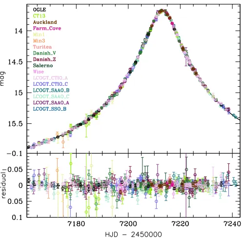
to the OGLE data without parallax is worse by Δχ2=10. After fitting the OGLE data with a point-lens model, we analyze the OGLE andSpitzerdata jointly. The parallax point-lens fit (Figure 2) shows significant systematic residuals in Spitzer but not in the OGLE data. Such a possibility was anticipated by Gould & Horne (2013), who suggested that space-based parallax observations might uncover planets that are not detectable from the ground because the spacecraft probes a different part of the Einstein ring. However, such a situation has never previously been observed.
The Spitzer residuals are qualitatively similar to those analyzed by Gaudi et al. (2002) for OGLE-1999-BUL-36. They found that this form of residuals could be explained either by a low mass-ratio companion (q 1) with projected separation (normalized to qE) s<1, or by light curve distortions induced by the accelerated motion of the observer on Earth, i.e., orbital parallax (Gould 1992). However, in the present case, the latter explanation is ruled out because the parallax is measured (and already incorporated into the fit) from the offsets in the observed(t0,u0)as seen from Earth and Spitzer,
p t b t
b
D D D º
-D º -
^
Å
Å
D
t t
t
u u
au
, ; ;
. 3
E, 0, 0,sat
E
0, 0,sat
( )
( )
Here, D^ is the Earth-satellite separation projected on the sky
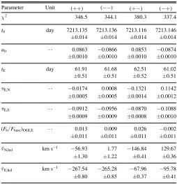
(changes from 0.84 to 1.31 AU over the course of Spitzer observations) and where the subscripts ⊕ and “sat” indicate parameters as measured from the Earth and the satellite, respectively. The four solutions are specified() according to the signs of u0 as seen from the Earth and Spitzer, respectively. See Gould (2004)for sign conventions. Table 2 lists four possible solutions, including the heliocentric
projected velocity,
p
p
= + Å ^ =
v v v v
t
; au, 4
hel geo , geo E
E 2
E
[image:5.612.320.569.49.293.2]˜ ˜ ˜ ( )
Table 1
OGLE-2015-BLG-0448 Point-lens Parameters Based on OGLE Data
Parameter Unit u0>0 u0<0
c2 125.1 125.0
t0 day 7213.153 7213.153
±0.016 ±0.016
u0 L 0.0874 −0.0876
±0.0016 ±0.0017
tE day 61.23 60.83
±0.84 ±0.95
pE,N L 0.113 0.180
±0.052 ±0.081
pE,E L −0.104 −0.111
±0.034 ±0.037
F Fb base OGLE
( ) L −0.002 −0.004
[image:5.612.42.295.74.268.2]±0.019 ±0.020
Figure 2.Point-lensfit(with parallax)toSpitzerand OGLE light curves of OGLE-2015-BLG-0448. The model(light blue line)fits the OGLE data(black points)quite well, but there are strong residuals in theSpitzerdata(red points and dark blue line), particularly near the start of the observations. The green line shows the planetary lens model for theSpitzerdata, which is discussed in the Appendix. The green long-dashed line in the lower plot shows the difference between theSpitzerpoint-lens and double-lens models.
Table 2
OGLE-2015-BLG-0448 Point-lens Parameters Based on OGLE and SpitzerData
Parameter Unit (++) (−−) (+-) (-+)
c2 346.5 344.1 380.3 337.4
t0 day 7213.135 7213.136 7213.116 7213.146
±0.014 ±0.014 ±0.014 ±0.014
u0 L 0.0863 −0.0866 0.0853 −0.0874
±0.0010 ±0.0010 ±0.0010 ±0.0010
tE day 61.91 61.68 62.51 61.02
±0.51 ±0.51 ±0.52 ±0.51
pE,N L −0.0174 0.0008 −0.1321 0.1142 ±0.0005 ±0.0005 ±0.0014 ±0.0012
pE,E L −0.0912 −0.0956 −0.0870 −0.1088
±0.0009 ±0.0009 ±0.0008 ±0.0010
F Fb base OGLE
( ) L 0.013 0.009 0.026 −0.002
±0.011 ±0.011 ±0.011 ±0.011
vN,hel˜ km s-1 −56.93 1.77 −146.84 129.67 ±1.30 ±1.22 ±0.41 ±0.36
[image:5.612.316.570.411.675.2]where vÅ ^, (N E, )= -( 0.6, 28.3 km s) -1 is the velocity of
Earth projected on the sky at the peak of the event. The(-+)
solution is preferred over the other ones byDc2=6.7because
OGLE data prefer pE,N>0 and this solution has the highest
pE,N. The comparison of Tables1and2shows that the OGLE
parallax measurement (which is based on slight light curve distortion)is consistent with the OGLE+Spitzerresult(which is based on the difference in t0 and u0 between the two observatories). Figure3displays the projected velocity vectors for these four solutions.
There are only three possible causes ofSpitzerpoint source, point-lens residuals: a binary(or planetary)companion to the lens, a binary companion to the source, or an unmodeled systematics in the light curve. Binary-source explanations for the residuals are basically ruled out by the fact that no sign of source binarity is seen in the OGLE light curve. Of course, one possible explanation for the lack of binarity effects would be an extremely red source, which has much lessflux in theIband than inSpitzerʼs 3.6μm that it simply does not show up in the OGLE data. However, the source is a red giant, so there are very few stars on the color–magnitude diagram(CMD)that are significantly redder. For two of the solutions(++and−−)in Table2, the source follows the same trajectory as seen from the Earth andSpitzer, just separated in time. Hence, binary-source solutions are obviously inconsistent with the OGLE data. For the other two solutions, the second source could pass farther from the lens as seen from the Earth compared toSpitzerby a factor » +1 (u0,sat+u0,Å) u0,sat¢»1 + 0.16 u0,sat¢ where
¢
u0,sat is the impact parameter of the source’s companion as seen bySpitzer. Given the slow development of the deviation,
¢
u0,sat 0.1, implying that this ratio of impact parameters is
2.6. The source is already close to the reddest stars on the CMD, hence the amplitudes of deviation have to be similar to the ratio of impact parameters, which is clearly ruled out by the
data. Notwithstanding these general arguments, we fit for binary-source solutions. We confirm that they are not viable. The binary-lens models with planetary mass ratio are discussed in theAppendix.
4. PROPER MOTION MEASUREMENTS
4.1. NGC 6558 Proper Motion Measurements in the Literature Thefirst measurement of the NGC 6558 proper motion was presented by Vásquez et al.(2013). Stars on the upper red giant branch (I<16.5 mag) and bluer than bulge giants were selected as cluster members and the mean proper motion of these stars was reported: mcl(N E, )=(0.060.14,
-0.52 0.14 mas yr) 1. The bluer red giants were chosen because the metallicity of the cluster stars is lower than the bulge red giants. Hence, cluster members on the giant branch are expected to be bluer. However, the bulge red giants show significant metallicity spread (Zoccali et al. 2008) and thus some bulge red giants can be mistaken for cluster members. Therefore, one expects the Vásquez et al.(2013)measurement to be biased toward smaller proper motion values. Additionally, the cluster proper motion relative to the bulge could be underestimated because cluster members may have been included in the ensemble used to establish the“bulge”frame. Rossi et al. (2015) published the only other NGC 6558 proper motion: mcl(N E, )=(0.470.60, -0.120.55)
-mas yr 1. In their approach, cluster member selection and frame alignment(needed for any proper motion measurement) were combined into one iterative process. The CMD decom-posed into cluster andfield stars can be used to diagnose the reliability of this process. The most prominent cluster feature on the CMD is the blue horizontal branch defined by the stars ofV>16 and(V-I)<0.9. The decomposed CMDs for the cluster and thefield reveal a very similar number of stars in this region, even though we do not expect field stars with these properties. The problems with decomposing blue horizontal branch stars suggests that the iterative process used to select cluster members and measure proper motions failed in this case.
4.2. NGC 6558 Proper Motion Measurement From the OGLE-IV Data
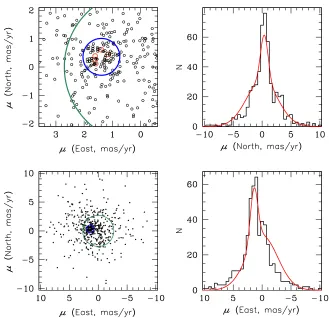
[image:6.612.48.288.52.277.2]We use two different methods to measure the proper motion of NGC 6558. In both cases, we make use of five years of OGLE-IV observations of this field. We first establish a “Galactic bulge reference frame”by identifying red giant stars from the CMD on the chip where the cluster lies, but excluding a circle of radius 1 52 around the cluster itself.54We note that for the immediate purpose of this paper, it is not important whether this reference frame is contaminated by non-bulge stars because we will measure the proper motion of the source in the same frame. However, the general utility of this measurement does require that this be the bulge frame, and the red giants are the best way to define this. Because the reference frame is defined by 2000 stars whose dispersion is about2.7 mas yr-1in each direction, it is randomly offset from the“true bulge frame”by0.06 mas yr-1in each direction.
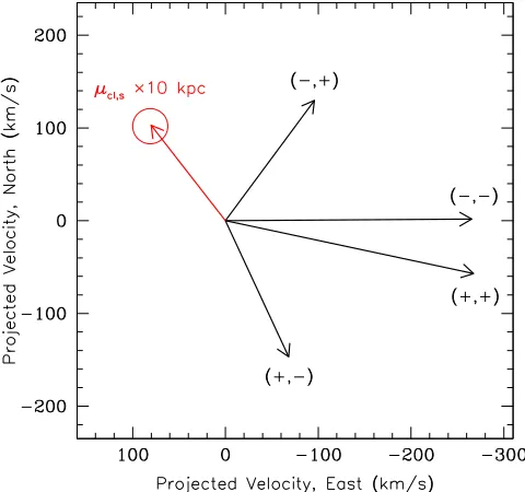
Figure 3.Comparison of directions of astrometrically measuredmcl,s(red)with
four degenerate projected velocities v˜hel based on microlensing data. The
proper motion measurement has been scaled by an arbitrary distance(10 kpc) so that it has the same units and approximately same size as the projected velocities. The direction ofmcl,sis inconsistent with any of the fourv˜hel. Hence,
the lens does not belong to the cluster.
54
In the first method, we measure the proper motion of each starI<18 magwithin a radius of 0 87 from the cluster center. We fit the resulting distribution of 518 proper motion measurements to the sum of two two-dimensional Gaussians, described by a total of four parameters, i.e., the cluster proper motionmcl, a single isotropic“cluster”dispersionσcl(actually mostly due to measurement error rather than intrinsic dispersion), and the fraction of all stars in the sample that belong to the cluster, p. The second Gaussian is assumed to have the same properties as the bulge population, i.e., a centroid at(0, 0)and a dispersion(2.7, 2.7 mas yr) -1.
Wefind p =243%,scl=0.65 mas yr-1, and
m N E, = +0.360.08,+1.390.08 mas yr .- 5
cl,1( ) ( ) 1 ( )
See Figure 4. The measured dispersion of cluster stars is significantly smaller than the dispersion of bulge stars. Hence, the cluster proper motion measurement depends only on stars in relatively small range of proper motions. The contribution of bulge stars to this part of the proper motion distribution does not significantly change with bulge dispersion.
In the second method, we measure the proper motions offive spectroscopically confirmed cluster members (Zoccali et al. 2008; Dias et al.2015), andfind
m N E, = +0.370.08,+1.470.09 mas yr ,- 6
cl,2( ) ( ) 1 ( )
where the error is determined from the scatter. See the upper left panel of Figure 4. Since these are consistent at 1σ, we combine the two measurements to obtain
m N E, = +0.360.06,+1.420.06 mas yr .- 7
cl( ) ( ) 1 ( )
We remind the reader that these errors are relative to the frame, which is what is relevant to our current application. Since the frame itself has errors of 0.06 mas yr-1, the total error in this value in the“true bulge frame”is0.08 mas yr-1.
4.3. Proper Motion of the Source Star
We measure the proper motion of the OGLE-2015-BLG-0448 source in the same frame:
m N E, = -1.810.40,-0.270.40 mas yr .- 8
s( ) ( ) 1 ( )
We estimate the error in two ways. First, we note that the two methods of measuring mcl revealed scatters of 0.65 mas yr-1 and 0.18 mas yr-1 for the two star samples with median brightness of I ≈ 17.2 mag and I ≈ 14.2 mag, respectively. Given that the OGLE-2015-BLG-0448 source has a baseline magnitude ofIbase=16.34, we adopt an intermediate value of
[image:7.612.140.469.46.364.2]
-0.40 mas yr 1. Second, substantial experience from regions where two OGLE fields overlap, shows that proper-motion errors are typically at about this level forI≈16.5 mag stars.
Figure 4.Proper motions of stars within0. 87¢ of the center of NGC 6558 based on OGLE-IV data. Left panels: vector-point diagrams. The distribution wasfit to the sum of two Gaussians, one for the bulge, centered at(0, 0)and with the known bulge dispersions=2.7 mas yr-1(green circle), and the other with freelyfit center
and dispersion(blue circle). This gives one measure of the cluster proper motion in the bulge framemcl(N E, )= +( 0.360.08,+1.390.08). In a second
method, we take the average proper motion offive spectroscopically confirmed cluster members(small red circles, upper left zoomed panel only), which yields mcl(N E, )= +( 0.330.08,+1.490.08). Since these are consistent, we combine them to yield Equation (7). Right panels: histograms of proper motion
The relative proper motion between the cluster and the source star is
m N E, = +2.170.40,+1.690.40 mas yr .- 9 s
cl, ( ) ( ) 1 ( )
4.4. The Lens Is Not a Cluster Member
We put the proper motion vector mcl,s (Equation (9)) on Figure3in order to test whether its direction is consistent with any of the lens-source projected velocities. Because mcl,s and
v˜hel have different units, mcl,s must be multiplied by a
dimensional quantity in order to be displayed on the same plot. We call this Drel for reasons that will become clear. We have chosenDrel =10 kpcsimply because the vectors are then
roughly the same size. Themcl,sis clearly inconsistent with any of the four values ofv˜hel, hence the lens is definitely not in the cluster.
However, ifmcl,s had been consistent with one of the v˜hel, then Drel required to make the two vectors in Figure 3 align would have provided an additional test for cluster membership. That is,
m = p
v
D au
, 10
l s
hel
, rel rel
˜
( )
where ml s, is the lens-source relative proper motion, which, for our purposes, can be taken as identical to the cluster proper motion because∣ml s, -mcl,s∣∣ml-mcl∣=vl,cl DL
-0.2 mas yr 1. Herev
l,clis the lens velocity in the cluster frame. If, for example, mcl,s had been in exactly the opposite direction to the one measured, it would have been consistent in direction with v˜hel,+-. Then, identifying the lens as in the
cluster would have impliedprel,cl,s100 asm . This would have
been an implausible value because the cluster is believed to be at D»7 kpc, i.e., pcl»140 asm , which would imply
ps=40 asm , i.e., DS =25 kpc. That is, the Drel required to alignmcl,s and v˜hel provides a powerful consistency check on the identification of the lens as a cluster member.
5. THE LOCATION OF THE LENSING SYSTEM
For a large fraction of past planetary microlensing events,qE is measured from thefinite source effects since the model then yields r=q q* E and the angular source radius q* is easily measured(Yoo et al.2004). Unfortunately, this event contains no caustic crossings or cusp approaches, so this standard method cannot be applied. Calchi Novati et al.(2015a)showed that for events with measured parallaxes pE, the lens distance
(and hence the mass) could be estimated kinematically, with relatively small error bars. However, of the 21 events analyzed there, all but 1 had projected velocities that either were quite large (v˜hel>700 km s-1)or were consistent in direction with
Galactic rotation. The first group are easily explained as Galactic bulge lenses prel0.02 mas, since m=v˜hel relp
p
= - v
-au 3 mas yr 1 700 km s 1 0.02 mas
rel
( ˜ )( ), which is a
typical value for bulge lenses. The second group are easily explained as lenses rotating with the Galactic disk, with the magnitude of v˜hel giving a rough kinematic distance estimate
*
prelmsgrA au v˜hel and msgrA*=6.38 mas yr-1 is the proper motion of SgrA*. The one exception was OGLE-2014-BLG-0807, for which the favored solutions hadv˜hel»200 km s-1.
The best model(-+)in Table2hasv˜hel=161.2 4 km s( ) -1,
while the models(++)and(−−)thatfit the data slightly worse
predictv˜hel=270 km s-1. Neither of thev˜helvectors is aligned with Galactic disk rotation, hence there is a low probability that the lens is in the Galactic disk. The measured projected velocity could be explained by a bulge lens if the lens-source relative parallax were larger than typical. The line of sight toward the event at Galactic coordinates(l b, )=(0 . 20, - 6 . 01) crosses the two arms of the bulge X-shaped structure(McWilliam & Zoccali2010; Nataf et al.2010; Gonzalez et al.2015). Hence, it is possible that the lens is in the closer part of the bulge and the source is much further away and the relative parallax is higher than typical. Even in this case the v˜hel=270 km s-1
solutions would be preferred over v˜hel=160 km s-1, i.e.,
contrary to the least-squares fits to the OGLE data. In either case, the most likely lens location is in the closer part of the bulge.
6. PLANET SENSITIVITY
With peak magnifications of 11(from ground)and 14(from Spitzer), and average cadences of 36 per day (ground-based survey plus follow-ups)and 6 per day(forSpitzer), the event OGLE-2015-BLG-0448 is among theSpitzer 2015 events that are most sensitive to planet perturbations. Therefore, we present the planet sensitivity of this event here, which will also be required for the determination of the Galactic distribution of planets, regardless of whether or not the planet detection in this event is real. Planet sensitivitySis defined as the probability of detecting a planet with the given properties: projected separation s (in units of Einstein ring radius) and mass ratioq.
We compute the planet sensitivity of this event using the method that wasfirst proposed by Rhie et al.(2000)and further developed by Yee et al.(2015)and Zhu et al.(2015)to include space-based observations. Details of the method can be found in the latter two references. In brief, wefirst measure the planet sensitivitySas a function ofqands. For each set of(q,s), we generate 300 planetary light curves that vary in angle between the source trajectory and the lens binary axis,α, but have other parameters fixed to the observed values. For each simulated light curve, we thenfind the best-fit single-lens model using the downhill simplex algorithm. The deviation between the simulated data and its bestfit, single lens model is quantified bycSL2 . For a subjectively chosen event, which is the case of OGLE-2015-BLG-0448, we first fit the simulated data that were released before the selection datetselectandfindcSL,select2 .
IfcSL,select2 >10, we regard the injected planet as having been noticeable and thus reject this α; otherwise, we compare cSL2 from the whole light curve with our pre-determined detection threshold, and consider the injected planet as detectable if cSL2 >c
threshold
2 . The sensitivity S q s
,
( ) is the fraction of α values for which the planet is detectable. We assume Öpik’s law in s, i.e., a flat distribution of logs, and compute the integrated planet sensitivityS(q).
dedicated follow-up observations of the anomalies and thus confirm these otherwise marginal detections. C2 as a supple-ment of C1 intends to capture the long-term weak distortions that may not show sharp deviations.
The calculation of planet sensitivity requiresρas an input. Here we estimate ρ following the prescription given by Yee et al.(2015):r=q q* EwhereqE =prel pE. The parallaxpEis well measured thanks to a combination of the OGLE and the Spitzerdata, hence below we need to estimate onlyprelandq*. The lens-source relative parallax can be easily found under the assumption that the lens is in the closer arm of the X-shaped structure and the source is in the farther arm. We follow Nataf et al. (2015), who modeled in detail the properties of the X-shaped structure in OGLE-III fields. The two centroids of RC luminosity functions corrected for extinction are
=
IRC1,0 14.210 mag and IRC2,0=14.715 mag for the event location(average values forfields BLG169 and BLG170). For the absolute RC brightness of MI,RC= -0.12 mag, the
corresponding distances are 7.3 and 9.3 kpc, hence,prel=0.028 mas.
To calculateq*, we assume the sourceI-band brightness and
-V I
( ) color are the same as the baseline object:
=
Is 16.337 mag and (V-I)s=1.589 mag (Szymanński
et al. 2011). This is justified because none of our models predicts significant blending. We corrected for extinction using Nataf et al. (2013) extinction maps and obtain:
=
Is,0 15.711 mag and (V-I)s,0 =1.046 mag. This
-V I s,0
( ) corresponds to (V-K)s,0 =2.419 mag (Bessell
& Brett 1988). The Kervella et al. (2004) color-surface brightness relation gives q*=3.4 asm . Finally,
*
r=q p pE rel=0.019and 0.011 for(-+)and(−−)models,
respectively.
We plot all the ground-based data in Figure5. The highest contribution to the planet sensitivity comes from the Auckland and LCOGT CTIO A data sets. We compute the planet sensitivity for two out of four possible solutions, (−−) and
-+
( ), and show the results in Figure6. Both solutions show substantial planet sensitivity (>10%) down toq =10-4. The
-+
( ) solution shows slightly higher sensitivity for
´
-q 2 10 4, mostly because observations taken from the satellite and the Earth are probing different regions in the Einstein ring, as has been discussed in Zhu et al. (2015); see also Figure7here for a demonstration. At smallestqvalues, the
-+
( )solution is less sensitive than the(−−)solution because the larger source size (r=0.019) smears out subtle features due to small planets. Figure7shows the detectability of planets with mass ratio q=1.70´10-4 as functions of planet positions for both investigated solutions. It is clear that the tentative planet detection reported here can only happen in the
-+
( )solution.
7. CONCLUSIONS
The event OGLE-2015-BLG-0448 presented a number of unique properties. It lay projected within tidal radius of the globular cluster. The maximum magnification reached was relatively high both forSpitzerand ground-based observations. It was also intensively monitored both from the ground and from space. All these properties made it a potential probe of the population of planets in globular clusters.
We analyzed the event photometry from both Spitzer and ground-based telescopes: the OGLE survey and follow-up networks of μFUN, RoboNet, and MiNDSTEp. Microlens parallax was measured using the difference in event properties as seen from the ground and space. The result confirmed the microlens parallax measured using only the OGLE data. Additionally, long-term astrometry of OGLE images were used to measure proper motions. We measured the proper motion of globular cluster NGC 6558 and the event source. Our analysis reveals that the lens could not be a cluster member. The same methods can be used for other potential cluster lens events that are observed by satellites.
We found that the Spitzer light curve reveals significant trends in residuals of the point-source point-lens model. The only two plausible causes of these trends are problems with Spitzer photometry or a planetary companion to the lens. We do not claim planet detection, but provide the results of planetary modelfitting in case the event photometry is proven to be correct.
The OGLE project has received funding from the National Science Centre, Poland, grant MAESTRO 2014/14/A/ST9/ 00121 to A.U. Work by W.Z. and A.G. was supported by NSF AST 1516842. Work by Y.S. and C.B.H. was supported by an appointment to the NASA Postdoctoral Program at the Jet Propulsion Laboratory, administered by Oak Ridge Associated Universities through a contract with NASA. Work by J.C.Y., A.G., and S.C. was supported by JPL grant 1500811. Work by J.C.Y. was performed under contract with the California Institute of Technology (Caltech)/Jet Propulsion Laboratory
[image:9.612.45.295.49.293.2](JPL)funded by NASA through the Sagan Fellowship Program executed by the NASA Exoplanet Science Institute. This publication was made possible by NPRP grant#X-019-1-006 from the Qatar National Research Fund (a member of Qatar Foundation). Work by S.M. has been supported by the
Strategic Priority Research Program “The Emergence of Cosmological Structures”of the Chinese Academy of Sciences Grant No. XDB09000000, and by the National Natural Science Foundation of China (NSFC)under grant numbers 11333003 and 11390372. M.P.G.H. acknowledges support from the Villum Foundation. This work makes use of observations from the LCOGT network, which includes three SUPAscopes owned by the University of St Andrews. The RoboNet programme is an LCOGT Key Project using time allocations from the University of St Andrews, LCOGT and the University of Heidelberg together with time on the Liverpool Telescope through the Science and Technology Facilities Council
(STFC), UK. This research has made use of the LCOGT Archive, which is operated by the California Institute of Technology, under contract with the Las Cumbres Observatory. Operation of the Danish 1.54 m telescope at ESOs La Silla observatory was supported by The Danish Council for Independent Research, Natural Sciences, and by Centre for Star and Planet Formation.
APPENDIX Tentative Planet
The point source modelfitted to theSpitzerdata resulted in residuals with significant trends. Here we discuss the possibility that these residuals were caused by the companion to the lens. The only possible binary-lens solutions must have planetary mass ratios q1 and projected separations s (in units of
Einstein ring) satisfying ∣s-s-1∣»0.5, i.e., logs» 0.11,
which follows from simple arguments. First, the source passes the lens atu0 »0.08as seen from both the Earth and Spitzer.
Since neither light curve is perturbed at peak, this already implies that the central caustic is small. Such small central caustics require eithers1,s1, and/orq 1. However, if either of the first two held, there could not be a significant perturbation at the point that it is observed atusat»0.5. That
is, the event timescaletE»60days is set by the unperturbed
OGLE light curve. Hence, the fact that the Spitzer curve experiences an excess roughly 30 days before peak implies that there is a caustic structure atusat»30 60 =0.5.
Thus, q1. In this planetary regime, such caustics occur when the planet is aligned to one of the two unperturbed images of the primary lens at u=∣s-s-1∣, i.e.,
= - +
s ∣ u (u2 4)1 2∣ 2. Hence,∣logs∣»0.11.
Finally, the fact that theSpitzerlight curve is perturbed while the OGLE light curve is not, implies(as in the above binary-source analysis)that the source passes on opposite sides of the lens(+-or-+solutions). The preference of(-+)in Table2 makes it the best solution.
[image:10.612.145.470.52.198.2]We consider four different topologies obeying the above constraints. First, s<1 with the source (seen by Spitzer) passing between the two triangular caustics for this topology. Second, s<1 with the source passing outside one of these caustics. Third,s>1. For each topology, we insert a series of seed solutions as a function of q and allow all parameters to vary. Wefind that thefirst and the third topologies never match
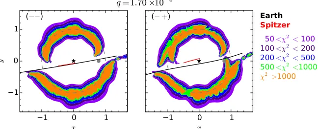
Figure 6.Planet sensitivity results of OGLE-2015-BLG-0448. The sensitivity as a function of two parameters,S q s( , ), is shown on the left panel, and on the right is shown the integrated sensitivityS(q)when aflat distribution ofsinlogsis assumed. In both panels, we show the sensitivities of the two solutions,(-+)(solid)and (−−) (dashed).
Figure 7. c2distributions of simulated OGLE-2015-BLG-0448 light curves with aq=1.7´10-4planet placed at different positions(x,y). The left panel shows the
result for the(−−)solution, and the right panel shows that for the(-+)solution. The black/red lines indicate the source trajectories as seen from the Earth/Spitzer. The lens is placed at(0, 0), and the position of the tentative planet is shown as afilled gray dot. Note that the tentative planet could only be detected in the(-+)
[image:10.612.145.469.251.383.2]the observed morphology of the Spitzer light curve because their relative demagnification zones do not align to the relative “dip” in the Spitzer light curve at about HJD¢ =7200. The second topology always converges to the same solution, which we present in Figure8. The modelSpitzerlight curve is shown in Figure 2 by a green line. The single lens parameters are consistent with the (-+) solution in Table 2:
=
t0 7213.161 14( ), u0= -0.0870 10( ), tE=61.16 16 d( ) , pE,N=0.1140 12( ), pE,E= -0.1088 10( ), and
=
F Fb base, OGLE 0.002 11( ). The additional binary-lens
para-meters are: a=189 . 71 25 ( ), s=0.7870 50( ), and
= ´
-q 1.70 32( ) 10 4. The c2 dof=209.7 331 is better by c2=127.7 than the point-lens solution, and better by
c
D 2=49 than the double-lens(+-) solution. We note that
even the best-fitting model does not remove all the systematics seen in theSpitzerresiduals.
The light curve lacks a close approach to the caustics, which is uncommon among published microlensing planets (Zhu et al. 2014). Without the caustic approach, we are unable to constrain the source size relative toqE. We note that Yee et al.
(2013)found a planetary signal below the reliability threshold in MOA-2010-BLG-311 event that also lies close to a globular cluster (NGC 6553 in that case).
REFERENCES
Bessell, M. S., & Brett, J. M. 1988,PASP,100, 1134
Bramich, D. M. 2008,MNRAS,386, L77
Bramich, D. M., Horne, K., Albrow, M. D., et al. 2013,MNRAS,428, 2275
Brown, T. M., Baliber, N., Bianco, F. B., et al. 2013,PASP,125, 1031
Calchi Novati, S., Gould, A., Udalski, A., et al. 2015a,ApJ,804, 20
Calchi Novati, S., Gould, A., Yee, J. C., et al. 2015b,ApJ,814, 92
Dias, B., Barbuy, B., Saviane, I., et al. 2015,A&A,573, 13
Dominik, M., Horne, K., Allan, A., et al. 2008,AN,329, 248
Dominik, M., Jørgensen, U. G., Rattenbury, N. J., et al. 2010, AN,331, 671
Gaudi, B. S., Albrow, M. D., An, J., et al. 2002,ApJ,566, 463
Gonzalez, O. A., Zoccali, M., Debattista, V. P., et al. 2015,A&A,583, L5
Gould, A. 1992,ApJ,392, 442
Gould, A. 1994,ApJL,421, L75
Gould, A. 2004,ApJ,606, 319
Gould, A., Carey, S., & Yee, J. 2014, Galactic Distribution of Planets from Spitzer Microlens Parallaxes Spitzer Proposal ID#11006
Gould, A., & Horne, K. 2013,ApJ,779, 28
Gould, A., & Loeb, A. 1992,ApJ,396, 104
Griest, K., & Safizadeh, N. 1998,ApJ,500, 37
Harris, W. E. 1996,AJ,112, 1487
Kervella, P., Bersier, D., Mourard, D., et al. 2004,A&A,428, 587
Kunder, A., Popowski, P., Cook, K. H., & Chaboyer, B. 2008,AJ,135, 631
Mao, S., & Paczyński, B. 1991,ApJL,374, L37
McWilliam, A., & Zoccali, M. 2010,ApJ,724, 1491
Nascimbeni, V., Bedin, L. R., Piotto, G., De Marchi, F., & Rich, R. M. 2012,
A&A,541, 144
Nataf, D. M., Gould, A., Fouqué, P., et al. 2013,ApJ,769, 88
Nataf, D. M., Udalski, A., Gould, A., Fouqué, P., & Stanek, K. Z. 2010,ApJL,
721, L28
Nataf, D. M., Udalski, A., Skowron, J., et al. 2015,MNRAS,447, 1535
Paczyński, B. 1986,ApJ,304, 1
Paczyński, B. 1994, AcA,44, 235
Refsdal, S. 1964,MNRAS,128, 295
Refsdal, S. 1966,MNRAS,134, 315
Rhie, S. H., Bennett, D. P., Becker, A. C., et al. 2000,ApJ,533, 378
Richer, H. B., Ibata, R., Fahlman, G. G., & Huber, M. 2003,ApJ,597, 45
Rossi, L. J., Ortolani, S., Barbuy, B., Bica, E., & Bonfanti, A. 2015,MNRAS,
450, 3270
Schechter, P. L., Mateo, M., & Saha, A. 1993,PASP,105, 1342
Skottfelt, J., Bramich, D. M., Hundertmark, M., et al. 2015,A&A,574, A54
Smith, M., Mao, S., & Paczyński, B. 2003,MNRAS,339, 925
Soszyński, I., Dziembowski, W. A., Udalski, A., et al. 2011, AcA,61, 1
Swift, J. J., Bottom, M., Johnson, J. A., et al. 2015, JATIS, 1, 2 Szymanński, M. K., Udalski, A., Soszyński., I., et al. 2011, AcA,61, 83
Udalski, A. 2003, AcA,53, 291
Udalski, A., Szymański, M., Kałużny, J., et al. 1994, AcA,44, 317
Udalski, A., Szymański, M. K., & Szymański, G. 2015, AcA,65, 1
Vásquez, S., Zoccali, M., Hill, V., et al. 2013,A&A,555, 91
Yee, J. C., Gould, A., Beichman, C., et al. 2015,ApJ,810, 155
Yee, J. C., Hung, L.-W., Bond, I. A., et al. 2013,ApJ,769, 77
Yoo, J., DePoy, D. L., Gal-Yam, A., et al. 2004,ApJ,603, 139
Zhu, W., Gould, A., Beichman, C., et al. 2015,ApJ,814, 129
Zhu, W., Penny, M., Mao, S., Gould, A., & Gendron, R. 2014,ApJ,788, 73
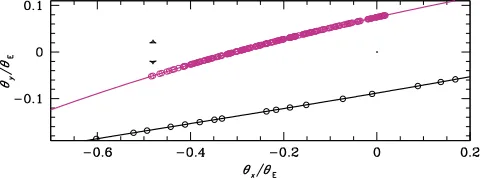
[image:11.612.49.290.53.142.2]Zoccali, M., Hill, V., Lecureur, A., et al. 2008,A&A,486, 177Z Figure 8.Source trajectory as seen fromSpitzer(violet)and the Earth(black).
The central caustic is located at(q qx, y)=(0, 0)and two triangular planetary
caustics are atq qx E= -s 1 s» -0.48. The circles indicate apparent source