Safe structural design for fatigue and creep using cyclic yield strength

SAFE STRUCTURAL DESIGN FOR FATIGUE AND CREEP USING

CYCLIC YIELD STRENGTH

Yevgen Gorash*_{and Donald MacKenzie}

Department of Mechanical and Aerospace Engineering, University of Strathclyde, Glasgow, Scotland, UK

ABSTRACT

This study proposes cyclic yield strength (CYS,σc

y) as a potential characteristic of safe design for structures operating under fatigue and creep conditions. CYS is defined on a cyclic stress-strain curve (SSC), while monotonic yield strength (MYS, σm

y) is defined on a monotonic SSC. Both values ofσc

yandσmy are identified using a 2-step fitting procedure of the experimental SSCs using Ramberg-Osgood and Chaboche material models. A typical S-N curve in stress-life approach for fatigue analysis has a distinctive minimum stress lower bound, the fatigue endurance limit (FEL,

σf

lim). Comparison ofσcy andσlimf reveals that they are approximately equal. Thus, safe fatigue design is guaranteed in the purely elastic domain defined by theσ_yc. A typical long-term strength (LTS) curve in time-to-failure approach for creep analysis has 2 inflections corresponding to theσ_yc

andσm_y. These inflections separate 3 sections on a LTS curve, which are characterised by different creep fracture modes and creep deformation mechanisms. Thus, safe creep design is guaranteed in the linear creep domain with brittle failure mode defined by the σc

y. These assumptions are confirmed using 3 structural steels for normal and high-temperature applications. The advantage of using σc

y for characterisation of fatigue and creep strength is a relatively quick experimental identification. The total duration of cyclic tests for a cyclic SSC identification is much less than the typical durations of fatigue and creep rupture tests at the stress levels around theσc

y. Keywords: Creep, Fatigue, Failure, Plasticity, Softening, Steel, Yield Strength.

INTRODUCTION

Characterisation of long-term strength of structural materials is an important engineering task for prevention of potential catastrophic failures of critical equipment. However, studies of this type are usually very long-lasting, technically challenging and involve expensive experimental work. Thus, the main scope of this study is the formulation of a simple way to predict characteristics of the long-term material behaviour (creep and fatigue, in the first instance) using basic material properties.

Based upon the extensive availability of experimental material data, a significant progress to-ward this challenge has been achieved so far and may be observed in the literature. Comparative study by Kimet al. [1] evaluated seven basic methods for estimating uniaxial fatigue properties (includingσf

lim) from tensile properties or hardness. This study was based upon the fatigue test data for eight ductile steels under axial and torsional loading. Three of the evaluated methods were able to predict over 93% of test cases within a factor of 3 compared with observed lives. The formulas forσf

limprediction included mechanical properties such as elasticity modulusE, ultimate tensile strengthσu and true fracture ductility εf. Among the variety of empirical formulations forσflim prediction with different combinations of aforementioned mechanical properties, the simplest are based onσu: σflim = 1.9018σu(Universal slopes method);σlimf = 1.5σu(Uniform material law); andσf

lim=σu+ 345MPa (Mitchell’s method), which shown an accuracy ofR2= 0.88. Another simple method in this comparison, proposed by Roessle & Fatemi [2], used a Brinnell hardness

HBfor prediction asσf_lim= 4.25HB+ 225MPa. This approach showed a reasonable accuracy ofR2= 0.86for experimental data fit.

The study by Casagrandeet al.[3] investigated a relationship betweenσf

limand Vickers hardness

HV in steels and developed a method to predictσf

lim. A good correlation was observed betweenHV andσf

limfor for four kinds of steels in different metallurgical states. However, the proposed empirical method is not straightforward and involves a number of parameters and equations to achieve a reasonable of accuracy ofσf

lim predictions. Recently, Bandaraet al. [4] proposed a formula for predictingσf

limof steels in the gigacycle regime. It uses a combination ofσuandHV as material parameters and was verified using the experimental results for 45 steels.

A different approach was developed by Liet al. [5], who estimated theoreticallyσc

yandσflim using test data for 27 alloy steels. One formula expressesσc

yby two conventional mechanical per-formance parameters –σ_u and the reduction in areaψ. The other formula expresses the FEL by the CYS with a reasonable accuracy ofR2 _{= 0.883as σ}f

lim = 1.13 (σyc)0.9. Despite the relative simplicity, the proposed relation can’t be considered as mathematically elegant, most probably be-cause of the conventional assumption of0.2% plastic strain offset forσc

yandσmy. Nevertheless, this formula by Liet al.[5] demonstrated the tendency thatσf

limis not too much different fromσyc. Less progress has been achieved in methods for creep rupture strength evaluation, but recently an important observation was discovered by Kimura [6]. The creep strength of ferritic and austenitic steels has been investigated in [6] through the correlation between creep rupture curve, presenting stress vs. creep rupture life, and 50% of 0.2% offset yield stress (half yield) at a wide range of temperatures. The inflection of the creep rupture curve at half yield was recognised for ferritic creep resistant steels with martensitic or bainitic microstructure, e.g. T91, T92 and T122. This was explained in terms of different mechanisms of microstructural evolution during creep at high- and low-stress regimes. The purpose of this study was to point out a significant risk of overestimation of long-term creep rupture strength by extrapolating the data for martensitic and bainitic steels (e.g. ASTM T91/P91) in high-stress regime to low-stress regime, which are separated by half yield.

A similar problem with particular application to ASTM P91 steel was investigated and discussed by Gorashet al. [7, 8] for the purpose of a creep constitutive model development. In these works, apart from inflection of creep rupture curve, the simultaneous inflection of the minimum creep rate curve, presenting minimum creep rate vs. stress, was recognised. Alternation of minimum creep rate slope was explained in terms of different creep deformation mechanism (linear creep for low stress and power-law for high stress), while alternation of creep rupture life slope was explained in terms of different damage accumulation modes (brittle fracture for low stress and ductile for high stress). The inflection of both curves was characterised by the same valueσ0called transition stress,

which had the meaning of material parameter in the developed “double-power-law” creep model. However,σ0was identified in [7, 8] using minimum creep rate data, and no relation ofσ0to basic

mechanical properties of ASTM P91 steel was recognised.

The principal aim of the present study is to investigate a link in characterisation of long-term strength of structural steel by finding a similar quantative feature in available experimental data. This establishes a straight relation between characteristics of creep and fatigue behaviour on one hand and yield strength as a basic material property and characteristic of plasticity on other hand.

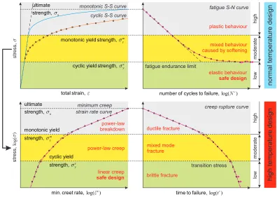
CONCEPT OF THE SAFE STRUCTURAL DESIGN

Definition of the yield strength

Dowling [9] discusses several methods to characterise the yield strengthσy. The first is the propor-tional limitσyp, which is the stress where the first departure from linearity occurs. The second is the elastic limitσel

y, which is the highest stress that does not cause plastic deformation. The third is the offset yield strengthσ0.2%

fatigue S-N curve

log( ) number of cycles to failure, N*

monotonic S-S curve

cyclic S-S curve

elastic behaviour safe design

total strain,e

stress,

s

mixed behaviour caused by softening

c y

cyclic yield strength,s _{fatigue endurance limit}

m y

monotonic yield strength,s

log( )t

time to failure, *

minimum creep strain rate curve

c log(&) min. creet rate, e

linear creep safe design power-law creep

creep rupture curve

brittle fracture mixed mode fracture

transition stress

plastic behaviour

ductile fracture

stress,

log(

)

s

power-law breakdown

normal temperature design

high temperature design

m y

monotonic yield strength,s

c y

cyclic yield strength,s

u

ultimate strength,s

u

ultimate strength,s

low

moderate

high

low

moderate

high

Figure 1: Concept of the safe structural design for fatigue and creep using cyclic yield strength

of defining the yielding event for engineering metals. Therefore,σ0.2%

y is usually meant to define the yield strengthσy in the literature. However, here theelastic limitσyel, defined in the scope of unified Chaboche model [10, 11], is used as the yield strengthσy.

This study proposesσc

yas a key characteristic for the definition of safe design for engineering structures operating under fatigue and creep conditions, as illustrated in Fig. 1. It is conventionally defined in context of a cyclic stress-strain curve (SSC), which is obtained from results of cyclic tests for a number of different strain ranges. Each cyclic test produces a stabilised stress response, which is effected either by hardening or by softening depending on the type of steel. In the case of steels with a cyclic softening effect,σc_y separates the low stress range of purely elastic behaviour from moderate stress range of mixed elasto-plastic behaviour. Monotonic yield strengthσm

y, which is conventionally defined in context of a monotonic SSC, separates the moderate stress range of mixed elasto-plastic behaviour from the high stress range of purely plastic behaviour. Both values ofσm y andσc

yare identified using a 2-steps fitting procedure of the experimental S-S curves. The first step applies the Ramberg-Osgood material model, which produces basic smoothing and extrapolation, to the both monotonic and cyclic SSCs separately. The second step of fitting involves a typical rate-independent form of the Chaboche material model with 3 kinematic backstresses. Fitting the Chaboche model with two separate sets of material constants sequentially to the both SSCs provides the values ofσm

y andσycwith minimum offset from the elastic line as elastic limits.

Stress-strain curves fitting procedure

0 50 100 150 200 250 300 350 400 450

0 0.0025 0.005 0.0075 0.01 0.0125 0.015 0.0175 0.02 0.0225

S tre s s ( M P a ) Total strain elastic mono. data mono. fit cyclic data R-O cyclic Ch. cyclic σy cyclic

Figure 2: Fitting of monotonic and cyclic SSCs of ASTM A36 steel from [12] at RT

0 100 200 300 400 500 600 700 800 900

0 0.01 0.02 0.03 0.04 0.05 0.06 0.07 0.08 0.09

Stres s (M Pa ) Total strain elastic mono. data Ch. mono σy mono cyclic data R-O cyclic Ch. mono

σy cyclic

Figure 3: Fitting of monotonic and cyclic SSCs of AISI 4340 steel from [13] at RT

0 50 100 150 200 250 300 350 400

0 0.002 0.004 0.006 0.008 0.01

S tre s s (M P a ) Total strain elastic R-O mono Ch. mono

σy mono

cyclic data

R-O cyclic

Ch. cyclic

σy cyclic

Figure 4: Fitting of monotonic and cyclic SSCs of ASTM P91 steel from [14] at 550◦C

0 50 100 150 200 250 300

0 0.002 0.004 0.006 0.008 0.01

Stres s (M Pa ) Total strain elastic R-O mono Ch. mono

σy mono

cyclic data

R-O cyclic

Ch. cyclic

σy cyclic

Figure 5: Fitting of monotonic and cyclic SSCs of ASTM P91 steel from [14] at 600◦C

non-linear relationship between stress and strain in materials near their yield point. It is particularly useful for metals that harden or soften with plastic deformation showing a smooth elastic-plastic transition. The equations for the monotonic and cyclic SSCs are:

εtot= σ

E +

(_σ B

)1/β

and ∆ε tot

2 = ∆σ

2E + (

∆σ

2B )1/β

, (1)

where∆ε_tot is the total strain range and ∆σis the total stress range (MPa) for each cyclic test respectively; Bandβ are the R-O material parameters; and Young’s modulusE in MPa. Using the value ofE, the total strainεtot_{in the experimental curves is decomposed into elastic and plastic} strain. Then the plastic componentεp _{of strain is fitted using the the least squares method by the} following power-law relations, which are derived from the Eq. (1):

σ=B (εp)β and ∆σ 2 =B

(

∆εp

2

)β

Table 1: Fitting parameters of the Ramberg-Osgood model (1) for different steels and temperatures

Type of plastic Elasto-plastic constants

material response E(MPa) B(MPa) β σy(MPa) ASTM A36 RT cycl. 189606 1015.61 0.2362 – AISI 4340 RT cycl.∗ 193053 1897.94 0.5175 320 ASTM P91 RT mono.

215000 710 0.047 –

ASTM P91 RT cycl. 1180 0.155 –

ASTM P91 500◦C m.

180000 594 0.066 –

ASTM P91 500◦C c. 763 0.15 –

ASTM P91 550◦C m.

172000 482 0.054 –

ASTM P91 550◦C c. 613 0.144 –

ASTM P91 600◦C m.

158000 330 0.042 –

ASTM P91 600◦C c. 446 0.123 –

ASTM P91 650◦C m.

140000 269 0.071 –

ASTM P91 650◦C c. 343 0.125 –

∗_{Extended version of the R-O model (6) is used for data fitting.}

The resultant R-O fits for monotonic and cyclic curves are then used to identify the parameters for the Chaboche material model. The range of applicability for the R-O fit is usually quite narrow not exceeding 1% ofεtotdepending on the grade of curvature grade for a SSC.

The basic variant of the rate-independent Chaboche model [10, 11] is presented as a combination of nonlinear kinematic hardening and nonlinear isotropic hardening models. The model allows the superposition of several independent backstress tensors and can be combined with any of the available isotropic hardening models. Since in this study monotonic and cyclic SSCs are fitted separately only for the identification ofσ_y, only the kinematic hardening component is considered:

X =

N

∑

i=1

Xi, with X˙i=Ciε˙p−γiXip,˙ (3)

whereε˙p_{is the plastic strain rate, andp˙is its magnitude. The total backstressXin Eq. (3) is given} by the superposition of a numberN of kinematic backstressesXi with a corresponding evolution

equation initially proposed by Armstrong & Frederick [16] forX˙i, whereCiandγiare kinematic

material constants. Chabocheet al. [10] recommendedN = 3in order to provide a good fit of experimental SSCs, which include large strain areas. Therefore, three backstresses are considered in this study providing an excellent match of the R-O fit (1) for a whole range of strains.

The kinematic hardening constants (Ci,γi) andσy, which define the size of the yield surface, are identified as recommended in [11]. The cyclic SSC is fitted by the following relation:

∆σ

2 =σ c y+

N

∑

i=1 Ci

γi

tanh

( γi

∆εp

2

)

, (4)

which is obtained in [11] by integrating Eq. (3) and consideringεp _{≈const at the peak stresses for} strain-controlled cyclic loading. Relation (4) is valid for the cyclic curve after stabilisation of the hardening or softening effects. Constants (Ci,γiand cyclicσ_yc) are identified by automatic fitting

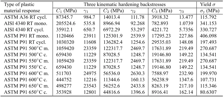
Table 2: Fitting parameters of the Chaboche model (3)-(5) for different steels and temperatures

Type of plastic Three kinematic hardening backstresses Yieldσ

material response C1(MPa) γ1 C2(MPa) γ2 C3(MPa) γ3 σy(MPa) ASTM A36 RT cycl. 87345.7 984.7 14013.4 111.78 3918.32 13.477 115.792 AISI 4340 RT mono. 205524.6 535.8 8966.94 92.268 782.893 1.0739 341.153 AISI 4340 RT cycl. 35912.1 650.7 6972.29 53.297 4221.72 5.7356 330.727 ASTM P91 RT mono. 1120466 23911 125301.9 2539.9 17295.23 227.86 406.098 ASTM P91 RT cycl. 1030320 11608 136282.4 1254.6 29535.03 148.08 197.493 ASTM P91 500◦C m. 1059420 23359 122317.7 2469.7 17631.89 219.49 270.687 ASTM P91 500◦C c. 659430 11229 87028.5 1248.7 19146.80 149.22 134.541 ASTM P91 550◦C m. 1059420 23359 122317.7 2469.7 17631.89 219.49 270.687 ASTM P91 550◦C c. 659430 11229 87028.5 1248.7 19146.80 149.22 134.541 ASTM P91 600◦C m. 511703 24975 56536.0 2630.3 7588.97 232.90 199.970 ASTM P91 600◦C c. 444752 12216 11344.6 160.13 56238.9 1347.6 107.731 ASTM P91 650◦C m. 498277 23543 56252.6 2433.8 8263.19 217.10 115.346 ASTM P91 650◦C c. 353928 12801 44816.6 1396.6 8916.41 162.14 80.6307

the decision variable cells containing material constants (Ci,γi andσcy) in order to minimise the value in the objective cell. This cell contains an average value of the absolute difference between columns containing ∆σ

2 calculated by Eq. (2) and Eq. (4) correspondingly in a particular range of

∆εp_{. Applying this approach, an excellent match of Eqs (2) and (4) is achieved.} The monotonic SSC is fitted by the different relation in the following form [11]:

σ=σ_ym+

N

∑

i=1 Ci

γi

[1−exp(−γiεp)], (5)

which contains the monotonicσm

y and different values of kinematic hardening constants (Ci,γi).

These constants are identified by fitting Eq. (5) to the R-O extrapolation (2) with “monotonic” values of the R-O parametersBandβ. The identification procedure is implemented in Microsoft Excel using an add-in Solver [17] in the same way as for cyclic SSC. An advanced step-by-step guideline for the estimation of the Chaboche viscoplasticity model parameters with their further optimisation was developed by Hydeet al.[18].

Application to three structural steels

The above described fitting procedure is applied to SSCs of three structural steels for the purpose of σm

y andσyc identification. The first is ASTM A36 steel, with mechanical properties reported in [19, 12], which is a standard low carbon steel, without advanced alloying and is a principal carbon steel employed for bridges, buildings, and many other structural uses. The monotonic SSC for this steel shown in Fig. 2 exhibits perfectly plastic behaviour when reaching the stress of36ksi= 248.211MPa in average, which is considered asσm

y. The perfectly plastic yielding lasts for approximately ofεp _{= 1(%) of strain plateau, which is followed by the strain hardening area,} then gradually approaching failure atεtot _{= 30(%). The cyclic SSC for this steel shown in Fig. 2} from [12] is fitted by the 2-step procedure, and the obtained material parameters for the R-O (1) and Chaboche (3)-(5) models are listed in Tables 1 and 2 correspondingly.

wider strain range than for the ASTM A36 steel. Therefore, the R-O model (1) is not able to provide an accurate fit of the cyclic SSC. In this case, the following modification of the R-O equation (1) is used for fitting analysis:

εtot= σ

E +

( σ−σy

B )1/β

and ∆ε tot

2 = ∆σ

2E + (

∆σ−σy 2B

)1/β

, (6)

Compared to Eq. (1), this notation contains an additional parameter of the yield strengthσ_yin the meaning ofσel

y, and can be applied for an accurate fitting of much wider strain range than Eq. (1). Thus, the cyclic SSC is fitted by the 2-step procedure. The obtained material parameters for the modified R-O (6) and Chaboche (3)-(5) models are listed in Tables 1 and 2 correspondingly.

The third material is ASTM P91 (modified 9Cr-1Mo) steel [20, 14], an advanced ferritic steel with martensitic microstructure, which has already been widely used over the last 2 decades as tubes/pipes for heat exchangers, plates for pressure vessels, and other forged, rolled and cast com-ponents for high temperature services. Both monotonic and cyclic SSCs shown in Figs 4 and 5 and mechanical properties at room temperature (RT), 500◦C, 550◦C, 600◦C and 650◦C are taken from [14]. Firstly, the monotonic SSCs are presented in [14] by the material parameters for the R-O model (1) listed in Table 1. The cyclic SSCs are presented in [14] by raw data, which is fitted by the R-O model (1) with material parameters listed in Table 1. Secondly, both monotonic and cyclic R-O extrapolations are fitted by the Chaboche model (3)-(5) with material parameters listed in Table 2.

RELATION IN MECHANICAL CHARACTERISTICS

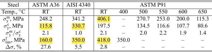
The next step is a check for possible correlations between the obtained yield strength values (σ_ym

andσ_yc) for ASTM A36, AISI 4340 and ASTM P91 steels and their fatigue and creep behaviour. This identifies a clear similarity for characteristic transition stresses in S-N fatigue, minimum creep strain rate and creep rupture curves, as explained below.

Fatigue behaviour at normal temperature

Engineering structures operating under cyclic loading conditions at normal temperature are usually designed against fatigue failure using the conventional stress-life approach. This approach involves experimental fatigue S-N curves with number of cycles to failureN∗vs. stress. A typical S-N curve is a straight line in double logarithmic coordinates with a distinctive minimum stress lower bound, which is called a fatigue endurance limit (FEL,σ_limf ). Referring to [9, 18],σ_limf is observed for a number of structural steels in benign environmental conditions and represents a stress level below which the material does not fail and can be cycled infinitely without fatigue damage. Comparison ofσc

ydefined as material constant and experimentally observedσlimf reveals that they are close. This assumption is confirmed by high-cycle fatigue (HCF) experimental data for ASTM A36 [21] and AISI 4340 [22, 23, 24] steels shown in Fig. 6. Comparison ofσf

limwithσycsummarised in Table 3 for ASTM A36 steel gives 27.6% accuracy and 5.5% accuracy for AISI 4340 steel. These observations indicate that safe fatigue design is guaranteed in the purely elastic domain defined byσc

y. Creep behaviour at elevated temperature

150 200 250 300 350 400 450 500 550 600 650

10000 100000 1000000 10000000

A

lterna

ting

s

tre

s

s

(

M

P

a

)

Number of cycles to failure

exp., Atlas of Fatigue Curves exp., Dowling (2004) exp., Ragab et al. (1989) exp., did not fail

4340 fatigue fit (σ_lim = 350MPa)

exp., Wang et al. (2010) traditional exp., Wang et al. (2010) energy

A36 fatigue fit (σ__{lim = 160MPa)}

Figure 6: S-N curve fits of ASTM A36 steel based on HCF data by Wanget al.[21] and AISI 4340 steel based on HCF data from Atlas of Fatigue Curves [22], Dowling [23] and Ragabet al.[24]

on the minimum creep rate curve, presenting minimum creep strain rate vs. stress, which is also a trilinear smoothed curve in double logarithmic coordinates. The deformations mechanism (linear creep, power-law creep and power-law breakdown) are separated by the same two inflections.

This assumption is confirmed by experimental observations for ASTM P91 steel at elevated temperatures. Data for creep rupture shown in Fig. 7 is all taken from the recent study by Kimura [6]. The inflections of corresponding curves were well observed at 600 and 650◦C and explained in terms of half monotonic yield (σ0_y.2%/2). In contrast to [6], in current study,σm_y andσ_ycfrom Table 2 are used in combination with test data [6] to provide a basic polylinear fitting. Data for min. creep strain rate shown in Fig. 8 is taken from studies by Skleničkaet al. [25], Kloc & Fiala [26] and Kimura [20]. The inflections of corresponding curves were observed at 550, 600 and 650◦C and explained in terms of transition between different creep deformation mechanisms. As in the case of creep rupture, here the sameσm

y andσycfrom Table 2 are used in combination with test data [20, 26, 25] to provide a basic polylinear fitting. Since the inflections are captured reasonably well on both types of data in Figs 7 and 8, the correspondence of transition stresses on creep rupture and min. creep rate curves proposed by Gorashet al. [7, 8] is proved by relating them toσm

y andσyc. It should be noted that Dimmleret al.[27] associated these inflections with microstructurally determined threshold stresses (back-stress concept). The applicability of this concept was shown using the experimental minimum creep rate and creep rupture curves for several 9-12%Cr heat resistant steels (P91, GX12, NF616, X20 and B2). Dimmleret al.[27] emphasised that the knowledge of these threshold stresses limits the range of experimentally based predictions, thus preventing from overestimation of long-term creep rate and creep strength from extrapolated short-term creep data. Therefore, these observations arise a consideration that the most safe creep design is guaranteed in linear creep domain with brittle failure mode, which is also defined by theσc

y.

10 100

100 1000 10000 100000

S

tre

s

s

(

M

P

a

)

Time to failure (h) exp., 500°C, Kimura (2013)

stress-based data fit, 500°C

exp., 550°C, Kimura (2013)

stress-based data fit, 550°C

exp., 600°C, Kimura (2013)

stress-based data fit, 600°C

exp., 650°C, Kimura (2013)

stress-based data fit, 650°C

cyclic yield σyc, all temperatures

monotonic yield σym, all temp.

Figure 7: Stress vs. creep rupture life of ASTM P91 steel based on the data by Kimura [6]

1.0E-09 1.0E-08 1.0E-07 1.0E-06 1.0E-05 1.0E-04 1.0E-03 1.0E-02 1.0E-01 1.0E+00 1.0E+01

1 10 100

Minimum

c

re

e

p

s

tra

in

ra

te

(1/

h)

Stress (MPa)

exp., 550°C, Kimura et al. (2009)

exp., 550°C, Sklenicka et al. (1994)

stress-based data fit, 550°C

exp., 600°C, Kloc & Fiala (2005)

stress-based data fit, 600°C

exp., 650°C, Kloc & Fiala (2005)

stress-based data fit, 650°C

cyclic yield σyc, all temperatures

monotonic yield σym, all temperatures

200 250 300 350 400 450 500 550

10000 100000 1000000 10000000 100000000

A

lterna

ting

s

tre

s

s

(

M

P

a

)

Number of cycles to failure exp., RT

exp., 400°C

exp., 550°C

exp., did not fail

RT fit (σ__{lim = 418MPa)}

400°_{C fit (}σ__{lim = 350MPa)}

550°_{C fit (no} σ__{lim exists)}

Figure 9: S-N curve fits of ASTM P91 steel based on HCF data by Matsumoriet al.[28]

From these data, it can be concluded that at elevated temperatures heat-resistant steels don’t exhibit

σf

limon S-N fatigue curves, which is usually observed at normal temperature. The reason for this is the elimination of purely elastic behaviour at high temperature, since there is always some amount of inelastic strain, which is caused by creep. Therefore, there is always a permanent accumulation of creep damage, even at low stress levels and high-strain rate, which leads to inevitable failure. This fact is confirmed by experimental observations [28], which demonstrated the extinction ofσf

limat 550◦C for over108_{loading cycles. However, a good match ofσ}f

limwithσmy with accuracy of 2.8% is observed at RT for this steel as shown in Table 3, which makes advanced martensitic steels different from simple ferritic steels is σf

lim prediction. This effect can be explained by the assumption of Terent’ev [29], who recognised two types of the fatigue endurance limitσf

lim– standard in HCF range (N = 102_-107_{cycles) and ultrahigh in gigacycle fatigue (GCF) range (N = 10}7_-1011_{cycles). The}

existence of ultrahighσ_limf was proved by the experimental data for high-strength steels (50CrV4, 54SiCrV6 and 54SiCr6), which demonstrated two inflections of the fatigue curves followed by horizontal plateaus – first in HCF area (N ≈105-106), second in GCF area (N ≈108-109). The correspondence ofσc_ywith ultrahighσf_limfor ASTM P91 steel is expected to be found atN >108 cycles, but no experimental data is available for this range.

CONCLUSIONS

Kimura’s [6] assumption of half monotonic yield (σ0.2%

y /2) agrees very well with the outcomes of the current study. According to Table 3, the relationσc

y≈σmy/2is valid for all temperatures except the highest 650◦C. This assumption is not relevant to AISI 4340 steel, which exhibitsσc

y≈σym. The principal advantage of theσc_yapplication to the characterisation of fatigue and creep long-term strength is the relatively fast experimental identification. The total duration of all cyclic tests, which are required to reach the stabilised stress response for the construction of cyclic SSC is much less than the typical durations of fatigue and creep rupture tests at stress levels aroundσc

Table 3: Comparison ofσm

y,σycandσflimfor ASTM A36, AISI 4340 and ASTM P91 steels

Steel ASTM A36 AISI 4340 ASTM P91

Temp.,◦C RT RT RT 400 500 550 600 650

σm_y, MPa 248.2 341.2 406.1 – 270.7 253.0 200.0 115.3

σc

y, MPa 115.8 330.7 197.5 – 134.5 116.6 107.7 80.6

σm

y/σyc 2.1 1.0 2.1 – 2.0 2.2 1.9 1.4

σf

lim, MPa 160.0 350.0 418.0 350.0 – – – –

∆σ, % 27.6 5.5 2.8 – – – – –

The critical point in the work presented here is an application of the advanced material model (i.e. Chaboche model [10, 11]) to the estimation of a single value of elastic limitσ_yel, which may seem to be complected. However, this approach is effective in typical cases when experimental SSCs are unavailable in explicit form, but available in the form of R-O [15] fittings (1). In other cases, when all necessary experimental SSCs are available in form of raw data, the modified form (6) of the R-O model may reduce the fitting procedure just to one step. Since Eq. (6) containsσ_yas a material parameter, the application of Chaboche model equations (3)-(5) is no longer needed.

REFERENCES

[1] Kim, K. S.et al.“Estimation methods for fatigue properties of steels under axial and torsional loading.” Int. J. Fatigue, vol. 24, no. 7, (2002), pp. 783–793.

[2] Roessle, M. L. and Fatemi, A. “Strain-controlled fatigue properties of steels and some simple approximations.” Int. J. Fatigue, vol. 22, no. 6, (2000), pp. 495–511.

[3] Casagrande, A. et al. “Relationship between fatigue limit and Vickers hardness in steels.”

Mater. Sci. & Eng. A, vol. 528, no. 9, (2011), pp. 3468–3473.

[4] Bandara, C. S. et al. “Fatigue Strength Prediction Formulae for Steels and Alloys in the Gigacycle Regime.”Int. J. Mater., Mech. & Manufacturing, vol. 1, no. 3, (2013), pp. 256–260. [5] Li, J. et al. “Theoretical estimation to the cyclic yield strength and fatigue limit for alloy

steels.”Mechanics Research Communications, vol. 36, no. 3, (2009), pp. 316–321.

[6] Kimura, K. “Creep rupture strength evaluation with region splitting by half yield.” Proc. ASME 2013 PVP Conf.PVP2013-97819, ASME, Paris, France (Jul. 14-18, 2013), pp. 1–8. [7] Gorash, Y. Development of a creep-damage model for non-isothermal long-term strength

analysis of high-temperature components operating in a wide stress range. PhD thesis, Martin-Luther-University Halle-Wittenberg, Halle (Saale), Germany (Jul. 21, 2008).

[8] Altenbach, H.et al. “Steady-state creep of a pressurized thick cylinder in both the linear and the power law ranges.”Acta Mechanica, vol. 195, no. 1-4, (2008), pp. 263–274.

[9] Dowling, N. E. Mechanical Behavior of Materials: Engineering Methods for Deformation, Fracture, and Fatigue. Pearson Education Limited, Harlow, UK, 4th ed. (2013).

[10] Chaboche, J.-L.et al. “Modelization of the strain memory effect on the cyclic hardening of 316 stainless steel.”Trans. 5th Int. Conf. on Structural Mechanics in Reactor Technology, no. L11/3 in SMiRT5, IASMiRT, Berlin, Germany (Aug. 1979), pp. 1–10.

[12] Higashida, Y. and Lawrence, F. V. Strain controlled fatigue behavior of weld metal and heat-affected base metal in A36 and A514 steel welds. FCP Report No. 22, University of Illinois, Urbana, Illinois, USA (Aug. 1976).

[13] Smith, R. W.et al.Fatigue behavior of materials under strain cycling in low and intermediate life range.Technical Note No. D-1574, NASA, Cleveland, Ohio, USA (Jan. 1963).

[14] Data sheets on elevated-temperature, time-dependent low-cycle fatigue properties of ASTM A387 Grade 91 (9Cr-1Mo) steel plate for pressure vessels. NRIM Fatigue Data Sheet No. 78, National Research Institute for Metals, Tokyo, Japan (Dec. 25, 1993).

[15] Ramberg, W. and Osgood, W. R. Description of stress-strain curves by three parameters.

Technical Note No. 902, NASA, Washington DC, USA (Jul. 1943).

[16] Armstrong, P. J. and Frederick, C. O. A mathematical representation of the multiaxial Bauschinger effect. Report No. RD/B/N731, CEGB, Berkeley, UK (Dec. 1966).

[17] MicrosoftrOffice Professional Plus. Excel Help System // Analyzing data // What-if analysis // Define and solve a problem by using Solver. Microsoft Corp., Release 2010 ed. (2009). [18] Hyde, T.et al.Applied Creep Mechanics. McGraw-Hill Education, New York, USA (2004). [19] ASTM Standard. Standard Specification for Carbon Structural Steel. A36/A36M – 08, West

Conshohocken, USA (2008).

[20] Kimura, K.et al.“Long-term creep deformation property of modified 9Cr-1Mo steel.”Mater. Sci. & Eng. A, vol. 510-511, (2009), pp. 58–63.

[21] Wang, X. G.et al. “Quantitative Thermographic Methodology for Fatigue Assessment and Stress Measurement.” Int. J. of Fatigue, vol. 32, no. 12, (2010), pp. 1970–1976.

[22] Boyer, H. E. Atlas of Fatigue Curves. ASM International, Materials Park, Ohio, USA (1986). [23] Dowling, N. E. “Mean Stress Effects in Stress-Life and Strain-Life Fatigue.” SAE Technical

Paper, , no. 2004-01-2227, (2004), pp. 1–14.

[24] Ragab, A.et al. “Corrosion Fatigue of Steel in Various Aqueous Environments.” Fatigue Fract. Engng Mater. & Struct., vol. 12, no. 6, (1989), pp. 469–479.

[25] Sklenička, V.et al. “Creep Behaviour and Microstructure of a 9Cr Steel.” D. Coutsouradis

et al., ed.,Proc. Conf. Materials far Advanced Power Engineering 1994. Part I, Kluwer Aca-demic Publishers, Liège, Belgium (Nov. 3-6, 1994), pp. 435–444.

[26] Kloc, L. and Fiala, J. “Viscous creep in metals at intermediate temperatures.”Kovové Mater-iály, vol. 43, no. 2, (2005), pp. 105–112.

[27] Dimmler, G. et al. “Extrapolation of short-term creep rupture data – The potential risk of over-estimation.” Int. J. of Pressure Vessels & Piping, vol. 85, (2008), pp. 55–62.

[28] Matsumori, Y.et al. “High Cycle Fatigue Properties of Modified 9Cr-1Mo Steel at Ele-vated Temperatures.”Proc. ASME 2012 Int. Mechanical Engineering Congress & Exposition. IMECE2012-87329, ASME, Houston, Texas, USA (Nov. 9-15, 2012), pp. 85–89.