A Study of recent classification algorithms and a novel approach for biosignal data classification

Theses Thesis/Dissertation Collections

2010

A Study of recent classification algorithms and a

novel approach for biosignal data classification

Eyup Cinar

Follow this and additional works at:http://scholarworks.rit.edu/theses

This Thesis is brought to you for free and open access by the Thesis/Dissertation Collections at RIT Scholar Works. It has been accepted for inclusion in Theses by an authorized administrator of RIT Scholar Works. For more information, please [email protected].

Recommended Citation

A STUDY OF RECENT CLASSIFICATION ALGORITHMS AND A NOVEL

APPROACH FOR BIOSIGNAL DATA CLASSIFICATION

By

EYUP CINAR

Thesis Submitted to the Faculty of Rochester Institute of Technology in partial fulfillment of the

requirements for the degree of

MASTER OF SCIENCE

IN

ELECTRICAL ENGINEERING

Approved by

Thesis Advisor Dr. Ferat Sahin _____________________

Thesis Committee Dr. Daniel Phillips _____________________

Thesis Committee Dr. Athimoottil Mathew _____________________

Department Head Dr. Sohail A. Dianat _____________________

ROCHESTER INSTITUTE OF TECHNOLOGY

KATE GLEASON COLLEGE OF ENGINEERING

DEPARTMENT OF ELECTRICAL AND MICROELECTRONICS ENGINEERING,

ROCHESTER, NEW YORK

A STUDY OF RECENT CLASSIFICATION ALGORITHMS AND A NOVEL

APPROACH FOR BIOSIGNAL DATA CLASSIFICATION

I, Eyup Cinar, hereby grant the permission to the Wallace Library of the Rochester Institute of

Technology to reproduce my thesis in whole or in part. Any reproduction will not be for

commercial use or profit

Acknowledgments

I am very grateful to my advisor Dr. Ferat Sahin for his generous support in my research and

academic life as well as the friendship developed over the past two years at RIT. I am thankful

to Dr. Daniel Phillips and Dr. Athimoottil Mathew for accepting to be a member of my thesis

committee and for their significant reviews and ideas for my thesis. I owe many thanks to my

family members for their endless motivation and encouragement throughout my studies abroad. I

am also very thankful to my colleagues Ryan Bowen, Ticiano Torres-Peralta, and Vince Baier

for their support for my research and their close friendships throughout my student life at RIT.

Last but not least I acknowledge the Fulbright commission of Turkey for providing me all the

List of Publications

Below is the list of publications resulted from this thesis work.

[1] E. Cinar and F. Sahin, “A Study of Recent Classification Algorithms and a Novel Approach

for EEG Data Classification,” in IEEE 2010 International Conference on Systems, Man and

Cybernetics, October 2010.

[2] E. Cinar and F. Sahin, “EOG Controlled Mobile Robot Using Radial Basis Function

Networks,” in IEEE Fifth International Conference on Soft Computing, Computing with Words

and Perceptions in System Analysis, Decision and Control (ICSCCW 2009), September 2009.

[3] R. Bowen, E. Cinar, and F. Sahin, “System of Systems Approach to a Human Tracking

Problem with Mobile Robots using a Single Security Camera,”in IEEE Fifth International

Conference on Soft Computing, Computing with Words and Perceptions in System Analysis,

Abstract

Analyzing and understanding human biosignals have been important research areas that have

many practical applications in everyday life. For example, Brain Computer Interface is a

research area that studies the connection between the human brain and external systems by

processing and learning the brain signals called Electroenceplograhpy (EEG) signals. Similarly,

various assistive robotics applications are being developed to interpret eye or muscle signals in

humans in order to provide control inputs for external devices. The efficiency for all of these

applications depends heavily on being able to process and classify human biosignals. Therefore

many techniques from Signal Processing and Machine Learning fields are applied in order to

understand human biosignals better and increase the efficiency and success of these applications.

This thesis proposes a new classifier for biosignal data classification utilizing Particle Swarm

Optimization Clustering and Radial Basis Function Networks (RBFN). The performance of the

proposed classifier together with several variations in the technique is analyzed by utilizing

comparisons with the state of the art classifiers such as Fuzzy Functions Support Vector

Machines (FFSVM), Improved Fuzzy Functions Support Vector Machines (IFFSVM). These

classifiers are implemented on the classification of same biological signals in order to evaluate

the proposed technique. Several clustering algorithms, which are used in these classifiers, such as

K-means, Fuzzy c-means, and Particle Swarm Optimization (PSO), are studied and compared

with each other based on clustering abilities. The effects of the analyzed clustering algorithms in

the performance of Radial Basis Functions Networks classifier are investigated. Strengths and

weaknesses are analyzed on various standard and EEG datasets. Results show that the proposed

classifier that combines PSO clustering with RBFN classifier can reach or exceed the

applied to a real-time system application where a mobile robot is controlled based on person‟s

Table of Contents

Acknowledgments... ii

List of Publications ... iii

Abstract ... iv

Table of Contents ... vi

List of Figures ... ix

List of Tables ... xi

1. Introduction ... 1

1.1 Motivation ... 1

1.2 Biological Signals and Their Characteristics: ... 4

1.2.1 Electroocculogram (EOG) Signals ... 4

1.2.2 Electroencephalogram (EEG) Signals: ... 6

1.3 Preprocessing ... 10

1.4 Feature Extraction ... 11

2. Clustering and Classification ... 14

2.1. Clustering Algorithms ... 15

2.1.1 K-means Clustering Algorithm ... 16

2.1.2 Fuzzy C-means Clustering Algorithm ... 17

2.1.3.1 Inertia Particle Swarm Optimization ... 22

2.1.3.2. Constriction Particle Swarm Optimization ... 23

2.1.3.3 PSO Clustering... 24

2.2. Classification Algorithms ... 26

2.2.1 Radial Basis Function Networks ... 26

2.2.2 Fuzzy Functions Support Vector Classifiers (FFSVC) ... 31

2.2.3 Improved Fuzzy C-Means Algorithm and Improved FFSVC (IFFSVC) ... 33

3. Results and Comparisons ... 35

3.1 Standard Datasets and Feature Extraction Method for EEG Datasets ... 35

3.2 Comparison of Clustering Methods ... 38

3.2 Comparison of Classification Methods ... 45

3.2.2 Results of FFSVC and IFFSVC Algorithms ... 46

3.2.3.1 Exhaustive PSO-RBFN ... 49

3.2.3.3 Hybrid PSO-RBFN ... 53

3.2.3.3 Pure PSO-RBFN ... 58

3.2.3.4 PSO Fuzzy Functions Support Vector Classifier ... 60

4. Applications and Experiments ... 64

4.1 Electroocculogram Controlled Mobile Robot ... 64

4.1.1 Training of the System and Decision Making ... 70

4.2 MediTrack Software ... 76

4.3 Real-Time Brain Computer Interface Application ... 80

4.3.1 The Emotiv Epoc Headsets ... 81

4.3.2. Hardware Specifications of the Headset ... 84

4.3.3 Software Development Kit (SDK) Libraries ... 85

4.3.5 Real Time Training, Testing, and the GUI Design ... 86

4.3.6. Robot Control with the Designed BCI ... 90

5. Conclusions ... 92

List of Figures

Figure 1 Components of Processing Biosignals ... 3

Figure 2 Polarization of the Eye Ball and an Example Electrode Placement for EOG Signal Collection [8] ... 5

Figure 3 Raw EOG data collected by Clevemed BioRadio 150 Data Acquisition Device as a Result of Repeated Rye Movement in a Left/Right Fashion by a Volunteer ... 6

Figure 4 (A) International 10-20 EEG Electrode Placement System. (B) Two EEG Traces Example with a Burst of Epileptiform Activity on the Posterior Right Side. P8-FCz represents subtraction of the signal FCz from electrode P8 [9] . ... 7

Figure 5 Mu Rhythm, Event Related Desynchronization, and Synchronization [11] ... 9

Figure 6 The Effect of Overlapping in Clustering Depending on the Fuzzification Constant m, x-y Axis represents the Cartesian Coordinates of Randomly Generated Data Points [33] ... 19

Figure 7 Radial Basis Function Networks Structure, Xn represents the nth Feature of Data, represents the ith Hidden Layer Kernel, Wm represents the weight of the mth link between Hidden and Output Layer, y represents the output of RBFN network ... 27

Figure 8 (A) Inputs Patterns in x-y coordinate system that form the XOR Problem (B) The Transformed Input Patterns into space using two Gaussian Kernels ... 28

Figure 9 Fuzzy Functions Support Vector Classifier Schematic [49] ... 32

Figure 10 Informative timing schematic for signal collection in the EEG dataset ... 37

Figure 11 Quantization Error Plot for EEG O3VR Dataset ... 39

Figure 13 Fuzzy C Means versus PSO Clustering on Standard non-EEG Datasets ... 42

Figure 14 Fuzzy C-Means versus PSO Clustering Other Datasets ... 43

Figure 15 Radial Basis Function Networks Parameter Selection and Training Flowchart ... 52

Figure 16 EOG signal data collected from the same person at different times. The movements tested by the subject includes looking at center, left, center, right and center in turn [61] ... 65

Figure 17 Electrode Placement for EOG Data Signal Collection [8] ... 66

Figure 18 Raw EOG Data and Low Passed Filtered Data ... 68

Figure 19 Part of the EOG Signal after Linear Regression ... 69

Figure 20 Structural Schematic for EOG RBFN Classifier ... 70

Figure 21 Determining Centers for the Hidden Layer Kernels by K-Means Clustering, dots represent the data points in the dataset and circles represent the cluster centers generated by K-Means Clustering ... 72

Figure 22 System GUI to Train and Control the Amigobot Robot, the crosses represent the moment that the decision has been made for the EOG signal [61] ... 73

Figure 23 Control Setup of the Mobile Robot ... 75

Figure 24 MediTrack Software GUI ... 79

Figure 25 The Emotiv Headset Control Panel ... 81

Figure 26 The TestBench Software Screen Capture ... 82

Figure 27 Electrode Positions of the Emotiv Headset ... 83

Figure 28 Software GUI Designed for Real Time System Training and Robot Control ... 86

Figure 29 Visual Stimuli by using the EmoCube ... 88

List of Tables

Table 1 Specific EEG Signal Frequency Ranges and Associated Real World Actions ... 8

Table 2 Specification of the Hidden Functions for XOR Problem ... 29

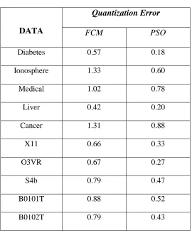
Table 3 Data and Quantization Errors ... 45

Table 4 Dataset Names and Corresponding Train, Validation, and Test Data ratios ... 47

Table 5 Fuzzy Function Support Vector Classifier Results ... 47

Table 6 Improved Fuzzy Functions Support Vector Classifier Results ... 48

Table 7 Exhaustive PSO-RBFN versus Exhaustive FCM-RBFN Classification Results ... 50

Table 8 Classification Performance for Hybrid PSO-RBFN with Quantization Error and RBF-Training Performance, µ: mean, Max: Maximum Performance Value, σ: Standard Deviation, Constriction Coefficient ... 55

Table 9 Classification Performance for Hybrid PSO with Quantization Error and RBF Training and Validation Performance (0.9T + 0.1V), µ: mean, Max: Maximum Performance Value, σ: Standard Deviation, Constriction Coefficient ... 55

Table 10 Performance Comparison of Different PSO Cost Functions ... 57

Table 11 Classification Results for Pure PSO-RBFN... 59

Table 12 PSO Fuzzy Functions Support Vector Classifier Results ... 61

Table 13 Best Performances of All the Classification Algorithms ... 63

Table 14 Classification of Network Outputs ... 71

Table 15 Patient Attributes ... 76

1. Introduction

1.1 Motivation

The human body generates several electrical signals that can be studied and analyzed to infer

some meaningful information for various applications. For example, human eyes generate a

signal called Electroocculogram (EOG) that could be used to determine the position of the

eyeball. The firing of many neurons due to neurological activities in the brain generates

Electroencephalogram (EEG) signals that might be helpful to decipher human thoughts or

intents. Similarly, the contraction of body muscles generates Electromyogram (EMG) signals

that could be used for the development of assistive devices.

With the advances in biomedical engineering and sensor technology, the analysis of human

bio-potential signals became a crucial research area. Researchers have been studying to understand

and classify human biosignals in order to provide various opportunities to people as in

developing assistive technologies for disabled people or obtaining more accurate diagnosis of

diseases.

For example, Greene et al. [1] uses the EOG signal measurements of schizophrenic patients and

tries to detect the disease utilizing saccade motions of the patients against a visual stimulus.

According to [1], these saccade motions of the eye can help detect the Schizophrenia disease in

humans. Suetsugu et al. [2] utilize the EOG signals in order to control a disabled person‟s

forearm by applying electrical stimulus to the arm muscles. Another study discusses generating

control inputs for a wheelchair by analyzing the human EOG signals and extracting the

directional information from the eyes so that the mobility of the severely disabled people might

In addition to EOG signals, examining the EEG signals might also help people by developing

assistive technologies for disabled people or obtaining more accurate diagnosis of brain related

abnormal activities. Lotte et al. surveys over 80 papers in terms of EEG classification techniques

for Brain Computer Interface applications [4]. In addition, Yuge et al. [5] studies the effects of

alcoholism on the EEG signals by extracting the power spectrum characteristics of the EEG

signal collected from the alcoholics in order to detect alcoholism on the patients.

As these studies [1-5] imply, the biological signals in human body might be effectively used to

make the human life easier through several applications. These types of studies have contributed

to new and rapidly developing scientific areas such as Cybernetics and Biorobotics [6].

According to Wiener, “Cybernetics is the science of control and communication in the animal

and the machine.” It merges humans and machines by utilizing intelligent tools in order to build

new systems that might make the human life easier [6]. On the other hand, Biorobotics is a field

that studies biological beings and how to mimic them to design new mechanical devices [7]. The

term is also defined as a subfield of robotics that studies biological beings to be a part of robots.

Considering the latter definition of Biorobotics and the definition of Cybernetics, we can

conclude that the main focus of these two fields is to develop a technology that might produce

inputs for the control of external devices and provide the interface between machines and the

human body.

In order to understand biological signals so that they could be used as inputs for the external

devices, one should go through several processes and make important considerations on several

components as shown in Figure 1. These components can be grouped into three main categories:

the data in order to remove undesired components in the signal that might be considered as

artifacts such as the eye blinks for the EEG signal. The second component is the Feature

Extraction that is extracting the features from the signal that might be discrimitive enough for the

human or machine to differentiate the signal into the different classes. The third component is

classifying the extracted features and determining the behavior, action, or thought which causes

the generation of the biopotential signal.

Biosignal Preprocessing Feature Extraction Classification

Figure 1 Components of Processing Biosignals

The main focus of this study is to contribute to the fields of Biorobotics and Cybernetics by

analyzing the strengths and weaknesses of the current state of the art classification and feature

extraction techniques, developing new and efficient ones that might increase the performance of

robust decision making, and applying these into the real world applications.

The following section includes a brief introduction on theoretical topics. It explains the nature of

the main biological signals examined in this study such as EOG and EEG and the important

1.2 Biological Signals and Their Characteristics:

Various electrical activities occurring in human body generate several signals called human

biopotentials. These signals can be recorded by utilizing special data acquisition devices and

interpreted by various processing and classification techniques to infer meaningful information.

In a very small scale, a biological ionic current is created by different polarization of specific

ions in a nerve cell such as sodium, potassium, and chloride. Considering the resistance of cell

membranes, the ionic current creates the electrical potential called a biopotential. There are four

types of human biopotential signals that have been studied by researchers. These are

Electrooculogram (EOG), Electromygram (EMG), Electrocardiogram (EKG), and

Electroencephalogram (EEG). The next two sections describe the EOG and EEG signals as they

are used in the applications described in this thesis.

1.2.1 Electroocculogram (EOG) Signals

The EOG signals are the biopotential signals generated by human eyes. Although there are many

theories about how the EOG signal is generated, the highly accepted theory is cornea-retinal

dipole theory [8]. According to this theory, the eye ball is polarized like a dipole as illustrated in

Figure 2 Polarization of the Eye Ball and an Example Electrode Placement for EOG Signal Collection [8]

Movement of the eye ball by the eye muscles changes the orientation of this dipole and generates

the EOG signal. This signal can be measured by the special electrodes placed on the specific

locations shown in Figure 2. While measuring the EOG signal, one electrode should act as

reference for the rest of the electrodes. This is usually selected away from the eyes and on the

forehead such as the location B in Figure 2.

In this study we use a data acquisition instrument called Bioradio 150 by Clevemed (Cleveland,

Ohio) ® for EOG signal collection. Figure 3 shows the raw EOG signal collected by this device

Figure 3 Raw EOG data collected by Clevemed BioRadio 150 Data Acquisition Device as a Result of Repeated Rye Movement in a Left/Right Fashion by a Volunteer

1.2.2 Electroencephalogram (EEG) Signals:

EEG signals are biopotentials recorded on the scalp, generated by the firing of the neurons in the

brain. It has been known that specific tasks in the human body are controlled by specific parts of

the brain and generated neurologic electrical activity is enough to be measured by the electrodes

placed on these specific parts of the brain [9], [10]. The recorded EEG signal by this method is

within 1-100 µV amplitude range and may contain useful information to decipher human

thoughts or intents. This information can be converted into control inputs for various systems

such as BCI-based assistive devices or detection systems for brain-related abnormal activities

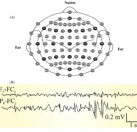
In order to collect EEG signals, electrodes are placed according to the standard International

10-20 system shown in Figure 4 (A). Each electrode is named with a letter to identify the brain

region and a number to identify the hemispheric location. For example, the letter F indicates that

the electrode corresponds to the Front region of the brain. The odd numbers refer to the left

hemisphere and even numbers refer to the right hemisphere of the brain [9].

(A)

(B)

Figure 4 (A) International 10-20 EEG Electrode Placement System. (B) Two EEG Traces Example with a Burst of Epileptiform Activity on the Posterior Right Side. P8-FCz represents

subtraction of the signal FCz from electrode P8 [9] .

Nasion

Figure 4 (B) represents an example of two EEG traces recorded from the human scalp for a 10

second epoch. It includes a burst of epileptiform activity at the end of the trace within the signal

recorded between P8 and FCz.

Certain frequency ranges of EEG signals have specific biological significance [10]. These typical

frequency ranges are named with Greek letter band names such as Alpha, Beta, Delta, and Theta.

It is known that some of the tasks controlled by the brain are more evident within specific

frequency bands [10]-[12]. Table 1 includes these standard frequency ranges of EEG signals,

their names, and examples of the bands in which specific actions are known to be more evident.

Table 1 Specific EEG Signal Frequency Ranges and Associated Real World Actions

Frequency Bands Evident Actions

Delta [0.5-4 Hz] Sleep waves in adults

Theta [4-8 Hz] consciousness slips towards drowsiness, deep mediation

Alpha [8-13Hz] Relaxed awareness without any attention and concentration

Beta [13-30 Hz] Active thinking, attention

Another important phenomenon with the EEG signals is known to be Mu rhythm or Event

Figure 5 Mu Rhythm, Event Related Desynchronization, and Synchronization [11]

This event is a characteristic attenuation in the power of EEG signal in certain frequency ranges

due to motor action preparation by the sensorimotor cortex area of the brain [11]. The

Sensorimotor cortex area is located in the central lobe of the brain and manages motor actions of

the body such as moving the arms or legs. Although this rhythm is observed in the planning stage

of physical movements, it has been discovered by Pfurtscheller [11] that it might also appear

when the human is shown a visual stimulus as a mental preparation of physical actions. This

visual stimulus is called Motor Imaginary. After an instant power decrease, the EEG signal

power increases again and this event is called Event Related Synchronization (ERS) as shown in

Considering the fact that particular parts of the sensorimotor cortex area in the brain control

different parts of the body, this phenomenon might help to detect and decipher human thoughts

regarding motor action intent in the brain.

As mentioned before, although there are other major types of human biopotential signals such as

EKG and EMG, their detailed explanations are not provided because their origin is not

considered as a relevant aspect of this study.

1.3 Preprocessing

The raw biosignal data collected from human body is usually contaminated with various noise

sources and artifacts. These undesired components might impact the efficiency of biological

signal processing techniques. Therefore various techniques are applied to the raw signal in order

to get rid of them and increase the efficiency of the Feature Extraction and Classification steps.

For example, the EOG signals created by eye blinks, Electrocardiogram, or Electromyography

signals from the facial muscles might all interfere with EEG signals. In addition to these

artifacts, various noise sources coming from the nearby electronic devices might also affect the

EEG signal.

The simplest but efficient technique in order to remove these undesired components is using

basic filtering. For instance, the most informative frequency range of EEG signal is within 0 Hz

and 30 Hz [10] thus the frequencies above 30Hz can simply be removed by a low pass filter. In

addition to these basic filtering, it is also possible to eliminate the noise from the original signal

using several different computational techniques such as Independent Competent Analysis (ICA)

or Principal Component Analysis (PCA) [9], [10].

In the Independent Component Analysis technique, the multisource signal is separated into

independent sub-components by considering the individual signals are statistically independent

[14]. In this way, assuming the noise source and the original data are independent, we can

separate the original signal from the noise. Vorobyov and Cichocki [15] apply ICA to separate

the EEG signal into independent components, and after filtering the noise they reconstruct the

clean EEG signal again.

Principal Component Analysis is one of the other computational techniques that could be used to

eliminate the noise and artifacts from the biosignal. PCA tries to reduce the dimensionality of the

signal into a smaller subspace which consists of orthogonal components that might enable the

separation of the original signal from its noise components [10]. Jung et al. [16] studied the

removal of artifacts from EEG signals by using and comparing both ICA and PCA techniques.

Depending on the nature of the signal and possible noise sources, one should select the best

preprocessing technique and apply it before the feature extraction phase. The following section

explains the feature extraction process and several techniques that are widely used in the

literature.

1.4 Feature Extraction

The second component of biological signal processing is to extract distinctive features that could

be a representation of the signal, discriminative enough to generate some meaningful

information. One of the common feature extraction techniques is employed by transforming the

original signal into frequency domain using Fourier Transform of the signal. For example, due

the time axis [17] and certain EEG frequency bands that have critical importance as mentioned,

the signal is transformed into the frequency domain. The Fast Fourier Transform (FFT) is

employed in order to generate the frequency domain representation of the signal and several

features are extracted after this transform. Nakayama et al. [17] uses the amplitude of FFT taken

EEG signals in order to generate the features. Felzer and Freisleben [18] uses FFT coefficients

between 5-15 Hz in order to obtain features for classification of EEG signals.

Principle Component Analysis is also used for feature extraction as well as it is used for noise

removing [19]. Since PCA downsamples the signal into principle components by utilizing its

eigenvectors, the eigenvalues associated with these eigenvectors can give useful information

about the signal. Lee et al. [19] uses PCA generated eigenvalues in order to train two different

classifiers for EEG signals.

In addition to FFT and PCA, the power of the signal in certain frequency ranges which is called

bandpower (BP) might also be used as features in the classification of biosignal. As mentioned

before for the EEG signals, certain events such as ERD cause the attenuation of the biosignal in

certain frequency ranges. This causes decreasing of the signal power in certain frequency ranges

[11] and could effectively be used in feature extraction as demonstrated by the researchers [4],

[20]-[23]. Bandpowers might also be used in obtaining features for the EOG signals. Estrada et

al. [24] studies classification of sleep stages and use bandpower of the EOG signal as features

since the Rapid Eye Movement (REM) activity is heavily concentrated on the frequency range

between 0.1 Hz and 0.3 Hz.

Depending on the requirements of the applications, it is possible to increase the number of

feature extraction methods for the biosignals. One should decide on the best feature extraction

method depending on the characteristics of the signal and the specific tasks or signals that are

studied. In this study, we have used the mean bandpower features within alpha and beta bands

for the EEG signals. These values are obtained by band-pass filtering the signal within specific

frequency ranges, squaring them and then taking the average. The reason to select BP values as

features for this study is the successful applications in the literature in classification of the EEG

signals [10-14] and the relevance of the technique for the events such as ERD that could be

detected by looking at the bandpower.

The next section gives detailed information about the third component in biological signal

processing called Classification. The theory and the literature review related to the classification

and clustering methods covered in this study are presented in section 2. Then, we discuss results

and comparisons in section 3. Finally, the applications and experiments are presented in section

2. Clustering and Classification

According to Alpaydin, “Machine learning is programming the computers to optimize a

performance criterion using example data or past experience” [24]. The software (or more

generally called the agent) analyzes the available data and tries to predict meaningful

information for the unseen data or extracts a description for the analyzed data. Machine learning

has been applied to the problems where there is no human expertise needed or unable to obtain

but still intelligent decisions can be made. For example, today‟s computers can recognize

spoken speech with a high success rate by utilizing Machine Learning techniques [26], [27].

Recognizing spoken speech is a difficult problem due to the highly varying nature of the signal

itself due to different accents, gender, and age. In this case, we cannot program the computers

directly to solve this problem. Some intelligent techniques are needed in order to understand

these signals and map them to the specific outputs. In summary, Machine Learning techniques

are applied to the most problems in order to develop systems that could make intelligent

decisions [24].

Machine learning techniques can be grouped into Supervised Learning, Unsupervised Learning

and Reinforcement Learning techniques [24]. Supervised Learning is learning a pattern from its

positive and negative examples and creating a mapping between the characteristic features of the

data into classes they belong. Unsupervised learning is used to model the data itself based on

only the input data without any supervisor. As a result of unsupervised learning, the obtained

model can give some idea about the organization of the data. For example, clustering algorithms

are considered within the group of unsupervised learning. They group the similar type of data

into clusters so that a model representing the structure of the data can be obtained.

environment and receives reward or penalty for its actions. First, all actions are equally important

for the agent and these actions are performed with the same priority in random selections. After

an action is performed, according to the type of the action, whether it is a desired or an

undesired, a reward or penalty is assigned to each action. Thus, the agent is reinforced to perform

a better action so that it may learn to behave in a more desirable fashion.

Throughout this study, several supervised and unsupervised learning methods have been

analyzed. In some cases these two learning methods have been combined to create hybrid

learning structures. Regarding the unsupervised techniques, the detailed analysis of clustering

algorithms has been made. The most frequently used clustering algorithms in the literature such

as Fuzzy C-Means, K-means, and Particle Swarm Optimization algorithms have been compared

based on their clustering abilities. After analyzing the strengths and weaknesses of these learning

techniques, they are used in the classification step and their effects on the classification accuracy

have been investigated.

The following sections explain the machine learning techniques (both clustering and

classification) analyzed or designed throughout this study.

2.1. Clustering Algorithms

In this section, we will study several clustering algorithms as methods of unsupervised learning.

The studied algorithms are K-means, Fuzzy C-means, and Particle Swarm Optimization

Clustering algorithms. The theory and literature related to these algorithms are presented, their

2.1.1 K-means Clustering Algorithm

K-means is one of the most common unsupervised learning methods that clusters the data

according to the centroids calculated as means of clusters. Each data member is assigned to the

nearest clusters by utilizing the Euclidean distance between the data and the cluster centroid. The

algorithm iteratively calculates the centroids of the clusters by minimizing the following

objective function

∑ ∑ ‖ ‖ (1)

which is a minimization of the sum of squared error distance from each data point to its cluster

centroid. In equation (1), represents the kth data point, represents the ith cluster centroid, n

is the total number of data points in the set, and c is the number of clusters that the data is desired

to be partitioned. The algorithm terminates when there is no change in the centroid locations or

equivalently in the objective function value.

The K-means algorithm pseudo code is as follows [24]

Assign c number of initial centroids for the clusters

While the change of centorid locations is greater than some epsilon value

Assign each data into the clusters using the minimum distance measures

For i=1 to c

Calculate the new centroid locations with the mean of all of the samples in the

cluster i

end While

Although K-means algorithm is simple and rapidly converging algorithm, it has a major

drawback. The algorithm might be trapped in local minima depending on the initial cluster

centroids which might avoid the algorithm to cluster the data well enough [28], [29], [30].

The authors in [28] propose a stochastic approach for K-means in order to alleviate the local

minima problem for the algorithm. The study in [29] similarly investigates the local minima

problem and proposes a technique by combining K-means clustering with Particle Swarm

Optimization (PSO) Clustering. They initially run the PSO clustering over the data and stop the

algorithm at some point according to the objective function value and let the K-means algorithm

run. However, deciding the specific value that the PSO algorithm should stop might be another

problem since it might highly vary according to the data being clustered. The authors in [30]

study the same drawback of K-means algorithm by initializing the centroids utilizing Genetic

Algorithms and apply this modification of the algorithm to an online shopping market

application.

2.1.2 Fuzzy C-means Clustering Algorithm

The aforementioned K-means clustering algorithm is known as a crisp clustering since portioning

of the dataset is performed according to the minimal distance calculation and each data is

classified into single cluster. However in Fuzzy C-means (FCM) clustering algorithm which is

first proposed by Dunn [31] and later developed by Bezdek [32], the data is partitioned into the

clusters according to their membership values. These values change between zero and one and

represent the degree of how close the data to each cluster center. In FCM algorithm, the data can

The Fuzzy C-means objective function is very similar to the K-means but it includes an

additional fuzzy term. The equation (2) represents the objective function of FCM algorithm,

∑ ∑ ‖ ‖ (2)

where represents the kth data entry in the dataset, represents the membership matrix, c is

the number of clusters, n is the number of data in the dataset, and is the ith cluster center.

According to [32], the following and formulas will minimize the above objective function.

∑ ⁄ (3)

∑

∑

where ‖ ‖ and represents the distance between the kth data entry and the ith cluster

center. The algorithm updates the cluster centers according to equation (4) and calculates the

membership matrix based on the new cluster centers. It terminates when ‖ ‖ that is

the cluster centroids do not change any more. The parameter m is called the fuzzification

constant. It adjusts the overlapping of the clusters [33] and is always greater than one. More crisp

clustering is obtained when m gets closer to one. As m gets larger, the overlapping of the clusters

is also increased. The effect of the fuzzification constant m on clustering is illustrated in Figure

Although FCM has advantages in clustering, such as the fast convergence and degree of

memberships which makes the clustering more realistic rather than crisp clustering, it also

suffers from various limitations. Cox [33] and Thomas et al. [34] explain several problems with

the algorithm. One of the limitations is that since the membership values depend on the other

cluster data points (partial membership), the cluster centers tend to move towards the center of

all the data points in order to increase the fuzziness. This is not a desired effect for the clustering

as explained by Wang et al. [35]. They explain that in order to obtain good partitioning of the

dataset, the fuzziness should be minimized as much as possible and the objective function of the

clustering algorithm should converge. The same problem with cluster centers in FCM algorithm

is also explained by [36] that proper location of the cluster centers is not the important focus of

FCM algorithm since the centers are moved according to the membership values of the data. In

addition, similar to the K-means algorithm converging to local minima based on different center

initializations may also exist with FCM algorithm as studied in [37].

Recently, Particle Swarm Optimization is being used for clustering by researchers based on its

performance in finding global solutions of optimization problems. The next section describes

PSO in detail and presents the state of the art PSO algorithm.

2.1.3 Particle Swarm Optimization (PSO) and PSO Clustering

Particle Swarm Optimization is an optimization technique inspired by social behaviors of bird

flocking and fish schooling developed by Kennedy and Eberhart [38]. Each particle in the swarm

is a potential solution to an optimization problem and has an associated fitness value calculated

by the fitness function to be evaluated. In every iteration of the algorithm, each particle is

allowed to update its position in the search space evaluating its own fitness and the fitnesses of

iterations is reached or there is no improvement in the global best solution of the swarm. The

particle which has the best fitness is selected as global solution at the end of the last iteration. For

each particle k in dimension d, velocity and position of particles are updated based on equations

(5) and (6).

( ) (5)

(6)

where;

current velocity of particle k

current position of particle k

best position of particle k

global best position of the swarm

cognitive weight

social weight

random number (0,1)

Below is a simple pseudo code of PSO algorithm [39]

Initialize Parameters

Initialize swarm

Find best particle

Find global best

Update velocity

Update position

end While

The random number term, r, in equation (5) causes the algorithm to explore the search space

continuously and thus help prevent the swarm from converging to a local solution. These

constant values in equation (5) together with the social and cognitive weights adjust the tension

in the swarm. The high values result in fast movements toward to the global solution passing

through the local solutions quickly [40]. Having random factors in the velocity update formula

might cause the swarm to explode and particles not to be able to converge to the global solution.

In order to avoid this situation, a maximum value for the velocity, vmax, is usually defined [38],

[39].

There have been several improvements and modifications to the standard PSO algorithm such as

Inertia PSO and Constriction PSO. The next two sections introduce these two types of PSO

modifications.

2.1.3.1 Inertia Particle Swarm Optimization

In the Inertia PSO, the current velocity of the particle is weighted with a constant Inertia Factor

w when the velocity is calculated for the next iteration [41]. Adding the Inertia Factor limits the

velocity of the particles so that an explosion effect can be prevented. Thus, The equation (5)

( ) (7)

This inertia factor might be a constant value throughout the algorithm or it might dynamically

decrease as the algorithm continues.

2.1.3.2. Constriction Particle Swarm Optimization

The other modification to the original PSO algorithm is the Constriction PSO [42] that we have

also utilized in this study. The Constriction PSO is a way to guarantee the convergence in the

system through the assignment of eigenvalues with a constriction coefficient determined by

cognitive and social acceleration coefficients. The velocity and position updates for this type of

PSO algorithm are shown in equations (8), (9) and (10)

( ) (8)

(9)

| √ | (10)

where;

Constriction constant

In equation (8), and are the cognitive and social constants as explained earlier. The

parameter, , is the parameter that determines the constriction constant . In [42], in order to

, (uniformly distributed random number between one and four) and

. The greater the constriction factor than 0.729, the faster the algorithm converges

however the probability of explosion might also increase.

Eberhart and Shi [42] proved that the Constriction PSO gives better results compared to the

Inertia PSO according to the experimental results obtained by examining five different objective

functions:. spherical, Rosenbrock, Rastrigin, Griewank, and Schalffer’s f6 function on sample

datasets. For our clustering implementation in this study, we have decided to use Constriction

PSO method. The next section introduces the application of PSO algorithm into the clustering.

2.1.3.3 PSO Clustering

Application of PSO into clustering was first proposed by Merwe and Engelbrecht in [43]. Each

particle in the swarm represents a potential solution for the clustering prototypes (centers) and

has a fitness value calculated by the objective function. In [43], the objective function is chosen

as the quantization error given in equation (11)

∑ ∑ | |

where | | represents the number of data vectors belonging to cluster j that is the frequency of

that cluster, represents the centroid of cluster j and is the pth data vector in the dataset and

is the number of clusters that the data will be partitioned.

When the quantization error formula in equation (11) is analyzed, it can be seen that the

quantization error is a measure of how close the centroid locations are to the data members in

each cluster. Since it makes the intra-cluster distances decrease and inter-cluster distances

[43]. Therefore, throughout this study, the clustering abilities of the algorithms are compared by

analyzing their abilities in reducing the quantization error in the dataset.

2.2. Classification Algorithms

In this section, the classification algorithms such as Radial Basis Function Networks, Fuzzy

Functions Support Vector Machines, and Improved Fuzzy Functions Support Vector Machines

that have been utilized throughout this study are presented.

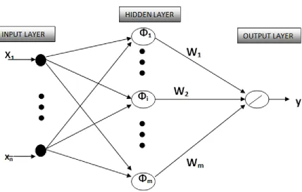
2.2.1 Radial Basis Function Networks

A Radial Basis Function Networks (RBFN) is a type of feed-forward Neural Network which

consists of three layers: input layer, hidden layer, and output layer as shown in Figure 7. The

input layer contains n dimensional feature vectors entering the network. The hidden layer is

composed of radially symmetric Gaussian kernel functions shown in equation (12)

‖ ‖

where and being the number of kernels, represents the ithkernel centroid in

the hidden layer, represents the feature vector in the dataset and values are calculated for

each data vector with kernel centroids determined by any clustering technique [44]. Note that,

the closer is to the higher the influence it will have in the hidden layer outputs since

Figure 7 Radial Basis Function Networks Structure, Xn represents the nthFeature of Data,

represents the ith Hidden Layer Kernel, Wm represents the weight of the mth link between Hidden

and Output Layer, y represents the output of RBFN network

By the help of the hidden layer, feature vectors which are in are mapped to a higher

dimensional space, , so that the data can more likely become linearly separable according to

Cover‟s theorem on the separability of random patterns [45].

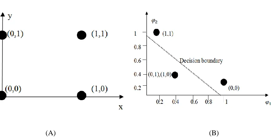
The most famous example that demonstrates the separability of patterns in higher dimensions is

the XOR problem [44]. The problem is constructing a classifier with the input patterns (1,1),

(0,1), (0,0), and (1,0) so that the classifier will give a binary output 0 when the input patterns are

(1,1) or (0,0) and the binary output 1 when the input patterns are (1,0) or (0,1). The input pattern

Figure 8.

(A) (B)

Figure 8 (A) Inputs Patterns in x-y coordinate system that form the XOR Problem (B) The Transformed Input Patterns into space using two Gaussian Kernels

As it can be seen from

Figure 8 (A), the input patterns (1, 1) and (0, 0) are not linearly separable from the other two

patterns. If the input patterns are mapped into another dimensional space by using two Gaussian

kernels, the input patterns turn out to be linearly separable as depicted in

Figure 8 (B). Table 2 shows the values of mapped input patterns in space where

Table 2 Specification of the Hidden Functions for XOR Problem

Input Pattern x Hidden Function Hidden Function

(1,1) 1 0.1353

(0,1) 0.3678 0.3678

(0,0) 0.1353 1

(1,0) 0.3678 0.3678

Thus, we may conclude that input patterns that are not linearly separable in their current space

might be transformed to a different or a higher input space by using kernel functions so that the

input pattern might become linearly separable.

As can be seen from Figure 7, in RBFN the outputs of the hidden layer are connected to the

output layer by weighted links. The output node of RBFN is a linear summation described in

equation (13)

∑ (13)

where Wj represents the weights of the links between hidden and output layers and is the

output of the mapping.

Let represent the value of the jth basis function, , for the ith data in the dataset. If there are

m inputs and m basis function units, the matrix form can be written in equation (14) to represent

[

] [ ] [ ] (14)

W Y

The weight matrix W can be calculated using the inverse of as stated in equation (15).

₍₁₅₎

When the number of inputs is greater than the number of hidden units, we can still find the

weight matrix utilizing the pseudo-inverse of the matrix. The pseudo inverse is calculated by

_.

During the testing phase of the data with RBFN, outputs are found by using the weights

obtained in the training phase and values calculated using only the test data. The outputs are

thresholded at the end in order to generate binary class label outputs.

In employing RBFN for a classification problem, finding the appropriate centers for kernel

functions has critical importance on the generalization capability of the classifier [46], [47].

K-means clustering algorithms have been widely used to determine the cluster centers for the

RBFN [44], [46], [47]. Although selecting these centers has critical importance, surprisingly not

many extensive studies do exist in the literature examining the importance of the clustering

algorithms on the classification performance [48].

Hongyang et al. [48] only studied the variation of K-means clustering using a dynamic K-means

According to the experimental results by [48], a better selection of the centers increases the

classification performance.

In this thesis document, two clustering algorithms on the classification performance of the RBFN

are explored and compared. In the next section, another classifier called Fuzzy Function Support

Vector Classifiers is introduced.

2.2.2 Fuzzy Functions Support Vector Classifiers (FFSVC)

The Fuzzy Functions Support Vector Classifier is a new classifier design proposed by

Celikyilmaz et al. [49]. It combines the Fuzzy C-Means Clustering Algorithm with any

classification methods to desig a new efficient classifier. With the conventional classifiers the

dataset, which has possible multi-model structure, is classified using a single classifier. This

might be a possible drawback for the classification tasks. The novel classifier approach captures

the hidden partitions in the dataset using FCM clustering and applies one classifier for each

partitions found by the clustering method.

Another important property of the technique is that the membership values found by FCM

clustering augment the original training feature set as a new dimension per each data. This helps

by increasing the dimensionality of the input space so that the data might more likely become

linearly separable. In addition, the data points that stay close to each other with opposite class

labels in the input space might move away from each other. Since the features of the data are

represented with one more additional feature, the identification of the data is also enhanced in the

The general structure of the classifier is represented in Figure 9. Let represent the membership

value of the input data in the training set belonging to the ith cluster and represents the jth

feature of the data vector where . Here, represents the feature dimension of

the dataset. After the FCM clustering is performed on the training data, a one dimensional input

matrix is created for each cluster partitioned by FCM. Here,

represents the augmented input vector that includes the membership value belonging to the ith

cluster. This input matrix is created for all clusters that the dataset is partitioned into.

Figure 9 Fuzzy Functions Support Vector Classifier Schematic [49]

Depending on the dataset, the transformation of these membership values might also be added as

additional feature in the input matrix together with the original membership values, e.g.

After the input matrices are created, one classifier for each cluster in the dataset is built.

Depending on the system, this classifier may take the form of a linear classifier such as a Logistic

Regression or a nonlinear classifier such as Support Vector Machine (SVM) [24]. These

classifiers that take the input matrix and generate a prediction for these input vectors are

called Fuzzy Classifier Functions (FCF). If a SVM is selected as the FCF, the output of these

Fuzzy Classifier Functions is the probability estimate of the class labels generated by Platt’s

probability approximation [51] represented by ̂ in Figure 9. Since this part of the FFSVC

method corresponds to the fuzzy if-then rules section in a Fuzzy Inference System (FIS) [52],

these functions are named Fuzzy Classifier Functions and the novelty of the classifier comes

from the property that the classifier can learn the fuzzy if-then rules from the data automatically.

The outputs of the FCFs are multiplied with the membership values in order to find a crisp

output as a result of the classifier. This part also corresponds to the defuzzification phase of

standard FIS. The result of the probability output is thresholded by 0.5 in order to generate

binary class outputs.

2.2.3 Improved Fuzzy C-Means Algorithm and Improved FFSVC (IFFSVC)

As we mentioned earlier, the membership values obtained from FCM clustering algorithm can be

used as additional predictors for the data during the classification. Celikyilmaz et al. [50]

proposed a modification to the standard FCM objective function by including the difference

between the class labels and a probability estimation coming from the Fuzzy Functions Classifier

to be minimized. This helps the FCM algorithm to optimize the membership values which could

better enhance the prediction for each dataset as discussed in the previous section. The modified

∑ ∑ ‖ ‖ ∑ ∑ ‖ ‖ | (16)

where the first term is the same as the objective function of the standard FCM and the second

term is the squared error of the difference between the actual class label and the probability

output of the ith Fuzzy Classifier Function (FCF) on the kth data, , as introduced in the

previous section. | represents the probability of the class output being equal to

one for the ith Fuzzy Classifier Function on the kth data in the dataset. The

| term in the objective function is called the error term.

It was proven in [50] that the membership update formula in equation (17) is the Lagrangian

multiplier of the objective function that can minimize the objective function in equation (16).

∑

where represents the Euclidean distance between the ith cluster center and the kth data vector.

Since the error term of the objective function in equation (16) does not include the cluster center

term, , the center update formula of the standard FCM stays the same.

Note that, in order to obtain the probability values for the membership update function, only the

initial membership values are used as feature vectors excluding the original data features for

the FCF. The probability estimates are performed according to the initial membership values.

These initial memberships can be obtained by running either the standard FCM or a crisp

The Improved Fuzzy Functions Support Vector Classifier (IFFSVC) uses this improved FCM

clustering algorithm in order to generate improved membership values for the data and classifies

them in the same way as FFSVC does.

3. Results and Comparisons

In this section, a comparison of different clustering and classification techniques, their

performance analysis, and a novel classification approach based on Particle Swarm Optimization

Clustering and Radial Basis Function Networks is presented.

3.1 Standard Datasets and Feature Extraction Method for EEG Datasets

There are two types of datasets used throughout this study for classification. The first type of

datasets is the standard datasets obtained from UCI Machine Learning Repository [53] such as

ionosphere, diabetes, liver, and cancer. These are two-class datasets that include various features

and a binary class label that refers the class of corresponding feature vector. The other type of

datasets is the standard EEG datasets such as X11, O3V, and S4b that include the EEG data for

different subjects. These are obtained from the BCI Competition IIIb [54]. The datasets B0101T

and B0102T also include the EEG data from the BCI Competition IV dataset 2b [55]. The

collection methods and the feature extraction method used to create these datasets are also

explained in detail later in this section. The Medical dataset contains statistical data related to

patients coming to the clinic provided by Bellevue Hospital in New York. In this dataset, there

are 19 features that include demographical attributes of each patient such as ethnicity, sex,

current diseases and additional binary class label representing whether the patient came to the

The EEG data used in this study is collected from different subjects at multiple sessions

including several runs each. The electrodes are placed according to International 10-20 system.

The positions placed on the scalp of subjects for each datasets are C3, C4 and Cz. The EEG

signal in datasets named X11, S4b and O3VR is sampled with 125 Hz and filtered between 0.5Hz

and 30Hz using a Notch Filter. These dataset names represent different subjects that the EEG

signal is collected. On the other hand, the EEG signal in the datasets B0101T and B0102T has a

sampling frequency of 250 Hz and filtered between 0.5 Hz and 100 Hz using a Notch Filter. The

data are collected according to motor imaginary pictures shown as cues.

Timing intervals for the collection of datasets is shown in Figure 10. One trial contains eight

seconds of recording. Shortly after a fixation cross is displayed on the screen, a short cue beep is

generated as a warning to the subject indicating that one of two visual cue images will be

Figure 10 Informative timing schematic for signal collection in the EEG dataset

Cue images displayed to the subjects on the screen are either left arrow or right arrow indicating

left thinking or right thinking. After the visual cue is displayed, through a virtual reality

experiment, feedback is given to the subject such as moving a ball to the left or right.

In order to extract features from these standard datasets, band power (BP) values of the signal are

used. The BP values extracted within alpha [8-13] Hz and beta [13-30] Hz frequency ranges as

suggested in [55] and [56]. The BP values are obtained by band-pass filtering the signal within

specific frequency ranges, squaring them and then taking the average. After generating BP

values, the mean band power value of the signal is calculated within the time interval of

feedback display. As a result of feature extraction, a four dimensional feature vector is obtained

within the alpha band from the electrode . Similarly represents the mean bandpower

value within the beta band from the electrode .

While the subject thinks left and right, due to different intensive neurological activity on the left

and right side of the brain, the band powers of the EEG signals measured from C3 and C4

electrodes also differ [57]. This can be discriminative enough to classify the left and right

thinking for the subjects.

3.2 Comparison of Clustering Methods

In the previous section, some drawbacks related to K-means and Fuzzy C-means algorithms were

discussed. In this section, experimental results are presented and algorithms are compared with

PSO clustering for their abilities to cluster the data using several standard datasets.

The reason that clustering algorithms are explored in terms of their abilities to do better

clustering is the critical importance of finding good cluster centers for the RBFN classifier as

proposed by Wettschereck et al. [58]. According to Wettschereck, learning the center locations

for RBFN hidden layer can better increase the generalization capability of RBFN classifier

therefore the chosen clustering algorithm may have high importance [58].

Three clustering algorithms are evaluated in their abilities to minimize the quantization error

given in equation (11). As it is discussed in the first section, minimizing the quantization error

can result more compact and better clustering in terms of the final clusters center locations.

Therefore the three algorithms are run on different standard datasets and their convergence plots

on these datasets are presented.

Figure 10 and Figure 11 show the convergence plots of the three clustering algorithms for their

obtained from [54]. The x-axis is the number of fitness evaluations, namely the evaluation of the

objective function.

Figure 11 Quantization Error Plot for EEG O3VR Dataset

0 100 200 300 400 500 600 700 800 900 1000

0 0.1 0.2 0.3 0.4 0.5 0.6 0.7 0.8 0.9 Q u a n ti z a ti o n e rr o r

Figure 12 Quantization Error Plot for EEG B0101T dataset

In these plots, the PSO algorithm is comprised of 100 iterations with 10 particles. In order to

make an objective comparison, since we know that the each particle evaluates the objective

function (quantization error in our case) one time in a single PSO step, the swarm with 10

particles in the PSO algorithm makes 10 fitness evaluations in one iteration. Therefore 100 steps

of the PSO algorithm means 100x10=1000 fitness evaluations per run. On the other hand, for the

FCM algorithm, since the membership and centroid update formulas are the Lagrangian

multipliers of the objective function and always try to minimize it, one iteration of FCM

0 100 200 300 400 500 600 700 800 900 1000

0 0.1 0.2 0.3 0.4 0.5 0.6 0.7 0.8 0.9 1 B0101T EEG

# Fitness Eval

corresponds to one time evaluation of the objective function. Therefore FCM and in the same

manner K-means algorithm are run 1000 fitness evaluations per run.

Plots in Figure 10 and Figure 11 verify that the PSO Clustering algorithm stops at a significantly

better location in terms of quantization error calculation than both the FCM and K-means

algorithms and converges to better minima for the analyzed datasets.

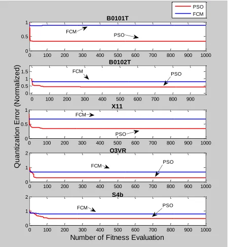
In addition to these, the performances of FCM and PSO clustering are also studied on the other

datasets. It is similarly shown in Figure 13 and Figure 14 that the PSO clustering algorithm

performs better clustering on the other datasets considering the 1000 fitness evaluations of both

Figure 13 Fuzzy C Means versus PSO Clustering on Standard non-EEG Datasets

0 100 200 300 400 500 600 700 800 900 1000

0 2

4 Medical

0 100 200 300 400 500 600 700 800 900 1000

0 0.5

1 Liver

0 100 200 300 400 500 600 700 800 900 1000

0.5 1

1.5 Cancer

0 100 200 300 400 500 600 700 800 900 1000

0 0.5

1 Diabetes

Number of Fitness Evaluation

Q

u

a

n

ti

z

a

ti

o

n

E

rr

o

r

(N

o

rm

a

liz

e

d

)

0 100 200 300 400 500 600 700 800 900 1000

Figure 14 Fuzzy C-Means versus PSO Clustering Other Datasets

Figure 13 and Figure 14 present important results on the compared clustering algorithms. The

first result that we can observe is due to the local minima problems of the FCM algorithm, no

matter how long we keep the algorithm running, there is no improvement in terms of clustering

0 100 200 300 400 500 600 700 800 900 1000

0 0.5

1 X11

0 100 200 300 400 500 600 700 800 900 1000

0 1

2 O3VR

0 100 200 300 400 500 600 700 800 900 1000

0 1

2 S4b

Number of Fitness Evaluation

Q

u

a

n

ti

z

a

ti

o

n

E

rr

o

r

(N

o

rm

a

liz

e

d

)

0 100 200 300 400 500 600 700 800 900 1000

0 0.5

1 B0101T

0 100 200 300 400 500 600 700 800 900