Dirichlet Bridge Sampling for the Variance Gamma Process: Pricing Path-Dependent Options.

City, University of London Institutional Repository

Citation

: Kaishev, V. K. and Dimitrova, D. S. (2009). Dirichlet Bridge Sampling for the

This is the accepted version of the paper.

This version of the publication may differ from the final published

version.

Permanent repository link:

Link to published version

: http://dx.doi.org/10.1287/mnsc.1080.0953

Copyright and reuse:

City Research Online aims to make research

outputs of City, University of London available to a wider audience.

Copyright and Moral Rights remain with the author(s) and/or copyright

holders. URLs from City Research Online may be freely distributed and

linked to.

City Research Online: http://openaccess.city.ac.uk/ [email protected]

process: pricing path-dependent options

Vladimir K. Kaishev, Dimitrina S. Dimitrova

Faculty of Actuarial Science and Insurance, Cass Business School, 106 Bunhill Row, London, EC1Y 8TZ, United Kingdom, [email protected], [email protected]

The authors develop a new Monte Carlo based method for pricing path-dependent options under the variance

gamma (VG) model. The gamma bridge sampling method due to Avramidis et al. (2003) and Ribeiro

and Webber (2004), is generalized to a multivariate (Dirichlet) construction, bridging ’simultaneously’ over

all time partition points of the trajectory of a gamma process. The generation of the increments of the

gamma process, given its value at the terminal point, is interpreted as a Dirichlet partition of the unit

interval. The increments are generated in a decreasing stochastic order and, under the Kingman limit, have

a known distribution. Thus, simulation of a trajectory from the gamma process requires generating only

a small number of uniforms, avoiding the expensive simulation of beta variates via numerical probability

integral inversion. The proposed method is then applied in simulating the trajectory of a VG process using

its difference-of-gammas representation. It has been implemented both in plain Monte Carlo and

Quasi-Monte Carlo environments. It is tested in pricing lookback, barrier and Asian options and shown to provide

consistent efficiency gains, compared to the sequential method and the difference-of-gammas bridge sampling

due to Avramidis and L’Ecuyer (2006).

Key words: option pricing; gamma bridge; Variance Gamma process; Dirichlet partitions; quasi-Monte Carlo; Kingman limit

1.

Introduction

Pricing path-dependent options whose underlying financial asset is driven by the so-called Variance Gamma (VG) process, introduced by Madan and Seneta (1990), has recently been considered by Ribeiro and Webber (2004), Avramidis et al. (2003) and Avramidis and L’Ecuyer (2006). These authors develop bridge methods for sampling from Gamma and Variance Gamma processes in Monte Carlo (MC) and Randomized Quasi-Monte Carlo (RQMC) environments, which demon-strate very good efficiency in estimating exotic option values. Developing such methods and

ing further their efficiency is of considerable practical importance, since different types of new and existing exotic derivatives are actively traded in the over-the-counter market and their fast and accurate pricing under the VG model has proved to be crucial. There are several advantages in assuming that a VG process is the driver of the underlying asset price. The VG process represents a pure jump L´evy process, constructed by randomly changing the time in a Brownian motion, following a gamma process with unit mean rate and certain variance rate. Such a random time change allows for modelling the flow of economically relevant time, reflecting the random speedups and slowdowns in real time economic and business activity. Choosing unit mean rate of the gamma subordinator guarantees the unbiasness of the random transformation of the time unit.

Another advantage of the VG process, pointed out by Madan et al. (1998), is that it offers much more flexibility in modelling skewness and kurtosis of the asset returns, compared to Brownian motion. As shown by the authors, once calibrated to market prices, the VG model captures volatility smile and fat-tailness of the asset return distribution. The modelling power and flexibility of the VG process has recently been emphasized by Carr et al. (2007). As they point out, the random change in time of the rate at which business news on stocks arrive, has a direct impact on the movement of their prices, hence on the volatility of the related option prices. Carr et al. (2007) highlight the ability of the VG process to successfully capture upward and downward jumps as well as infinitesimally small movements (jitters) in the underlying stock price.

The nice properties of the VG model have led to its recent implementation in the Bloomberg system, through the function SKEW. It allows for contrasting VG against Black-Scholes in pricing options, based on market data. No doubt, this important step will boost further the popularity of the VG model among financial analysts, traders and other practitioners. The importance of the VG model has been highlighted also in the growing number of publications devoted to its empirical and theoretical properties, computational methods and various financial applications. Among these are recent contributions by Yor (2007), Fu (2007), Carr et al. (2007), Daal and Madan (2005), Carr et al. (2002), to name only a few. All this suggests that exploring the VG model further and developing efficient methods for option pricing under VG becomes more and more relevant both from the practical and theoretical point of view.

Along with the above mentioned advantages, a difficulty in using a VG process, and more generaly a L´evy process, as driver of the price of the underlying asset is that they require more sophisticated stochastic analysis and in the case of path-dependent option pricing do not lead to closed-form solutions. Thus, in the latter case it has proved essential to develop efficient Monte Carlo based valuation methods. However, in general, a well known drawback of the plain Monte Carlo methods is their slow convergence, which can make the estimation process very time consuming if a precise estimator is required. Various techniques, among which control and antithetic variates, stratified sampling and QMC methods, have recently been used for efficiency improvement over the plain Monte Carlo. A detailed account on these techniques is to be found in Glasserman (2004). For a recent overview of Monte Carlo methods for sampling from the VG process see Fu (2007).

Sampling (BGBS). The same bridge technique for sampling from the VG process has been inde-pendently developed by Ribeiro and Webber (2004). Avramidis et al. (2003) and Avramidis and L’Ecuyer (2006) have also applied gamma bridge sampling to develop the Difference-of-Gamma Bridge Sampling (DGBS) method, based on the representation of the VG process as a difference of two independent gamma processes (see Madan et al. 1998). Both the BGBS and the DGBS methods utilize the fact that the gamma bridge sampling improves the efficiency of the QMC by concentrating the variance at the first few simulated random numbers, thus reducing the effective dimension of the valuation problem. However, these methods involve generating computationally expensive beta random variables via numerical probability integral inversion.

Our aim in this paper is to develop a new efficient Monte Carlo method for pricing path-dependent options, when the underlying asset is driven by a Variance Gamma process, which requires generation of uniform variates only. It is called Dirichlet bridge sampling (DirBS) and incorporates a multivariate (Dirichlet) generalization of the gamma bridge sampling. Our approach can be interpreted as a multivariate bridging ’simultaneously’ over all the partition points of the trajectory of a gamma process. It is based on the fact that the beta distribution defined by the two increments of the gamma bridge, generalizes to a Dirichlet distribution of the increments at all time partition points, of the gamma process, given its terminal value (see e.g. Wilks 1962 and Kotz et al. 2000, chapter 49). Furthermore, we view this Dirichlet distributed random vector of increments as a Dirichlet partition of the unit interval. Hence, the simulation of a trajectory of a gamma process is interpreted as a Dirichlet division of the unit interval. This important observation has allowed us to exploit the properties of the so-called size-biased permutation of the Dirichlet fragments of the unit interval, which represents a size-biased Dirichlet fragment selection procedure (see section 3.2). Thus, following this procedure, we generate the increments of a gamma process in a decreasing stochastic order.

L’Ecuyer (2006), in terms of efficiency in pricing Asian, barrier and lookback options. Comments and conclusions are provided in section 5.

2.

Pricing path-dependent options under the Variance Gamma model

2.1. Background

Assume the dynamics of the price of a financial asset is described by the risk neutral asset price process{S(t), t≥0},

S(t) =S(0) exp{(ω+r)t+X(t)}, (1) where X(t) =X(t;ϑ, σ, κ),t≥0 is a Variance Gamma (VG) process, r >0 is the risk free rate of interest and the constant ω= [ln (1−ϑκ−(σ2_{κ)/2)]/κ is chosen so that} E_{(S(t)) =S(0) exp}{rt}_,

i.e. the process exp{X(t)} is a martingale, which imposes the requirement (ϑ+σ2_{/2)κ <1 on the}

parameters of the VG process.

The VG process was first introduced by Madan and Seneta (1990) and developed further by Madan and Milne (1991) and Madan et al. (1998). It represents a Brownian motion W(t) =

W(t;ϑ, σ) with drift parameter ϑ∈R and variance parameter σ >0, in which the time variable is replaced by an independent gamma process G(t;α, λ) with parameters α >0 and λ >0, and density at tgiven by

fG(t;α,λ)(x) =

λαt

Γ (αt)x

αt₋1

e−λx, x >0,

where Γ (·) denotes the gamma function. The parameter αof a gamma process G(t;α, λ) controls the intensity of the jumps of all sizes simultaneously, whilstλcaptures the decay rate of big jumps. In the case of the VG processα=λ= 1/κ, so that the variance rate of the gamma subordinator is

κ >0 and its mean rate is unity.

It can be shown (see Madan et al. 1998) that the VG process can also be expressed as a difference of two independent gamma processes

X(t) =G0(t;α, λ0)−G1(t;α, λ1), (2)

with a common shape parameter α= 1/κand scale parameters

λ0 =

2

κ

(√

ϑ2₊2σ2

κ +ϑ

λ1 =

2

κ

(√

ϑ2₊2σ2

κ −ϑ

).

A recent overview of the properties of gamma processes, which appear as building blocks for the VG process, can be found in Yor (2007). In the sequel, we assume that a Variance Gamma model has been fitted to financial data and therefore, the values of the parameters of the VG process,

X(t;ϑ, σ, κ), have been determined (see e.g. Chan 1999, Seneta 2004 and Madan et al. 1998 for further details and ideas on how this can be done).

Now, consider the problem of pricing a contingent claim, such as an option contract, with payoff at maturity, T, given by

CT =f({S(t),0≤t≤T}),

wheref is some function of the stock price process (1). Then, the price at inception of the contract is

C0= ˆE

(

˜

CT )

,

where ˆE denotes the expectation under some risk neutral martingale measure ˆP, and ˜CT denotes

the terminal payoff discounted at the (possibly stochastic) risk free interest rate.

In reality, the process S(t) is observed at some fixed points in time 0 =t0< t1<· · ·< tN =T,

(or the payoff may depend on the value ofS(t) at a finite number of time epochs), therefore

CT=f(S(t1), . . . , S(tN)).

In order to estimateC0, the processS(t) is sampled at the time points 0 =t0< t1<· · ·< tN =T,

using Monte Carlo methods. By generatingM >0 sample paths,M values of the discounted payoff function, ˜cm

T,m= 1, . . . , M, can be calculated. The Monte Carlo estimate,c0, of the contract price

can then be obtained as

c0=

∑M

m=1˜c

m T

M . (3)

2.2. Bridge sampling of Gamma and VG processes

As described in the introduction, there are two bridge approaches to the construction of a sample trajectory X(t1), . . . , X(tN) of the VG process X(t), namely the BGBS method, which is based

on the representation of the process as a subordinated Brownian motion, and the DGBS method, which utilizes the representation (2) of the VG process. The core part of both approaches is the bridge sampling of a gamma processG(t;α, λ) which can be summarized as follows.

Given any three time points 0≤ti< tj< tk≤T and the values of the gamma process,G(ti;α, λ)

and G(tk;α, λ), atti and tk, respectively, consider the problem of generatingG(tj;α, λ). Let Y1=

G(tj;α, λ)−G(ti;α, λ) andY2=G(tk;α, λ)−G(tj;α, λ). Hence,Y1 and Y2 are mutually

indepen-dent, andY1∼Gamma(g1, λ),Y2∼Gamma(g2, λ), whereg1= (tj−ti)αand g2= (tk−tj)α.

Fur-thermore,Z=Y1+Y2=G(tk;α, λ)−G(ti;α, λ) isGamma(gZ, λ) distributed withgZ= (tk−ti)α.

It can be shown that the conditional density ofY1, given Z=z, is

fY_1|Z(y1|z) =

1

B(g1, g2)

(_y

1

z

)g1−1(

1−y1

z

)g2−1 z−1,

which implies that

G(tj;α, λ) =G(ti;α, λ) +bt_jz,

where btj∼Beta(g1, g2) and B(a, b) denotes the beta function.

Ribeiro and Webber (2004) show that the BGBS method, when combined with stratification at certain time points, leads to substantial efficiency gains, relative to plain Monte Carlo, despite the time-consuming generation of the beta random variables btj∼Beta(g1, g2) using the inverse

transform method. Avramidis et al. (2003) compare different algorithms for sampling from the VG process in Monte Carlo (MC) and Quasi-Monte Carlo (QMC) environment and show that generally, DGBS gives the maximal variance reduction, but BGBS often leads to higher efficiency gains. The latter is again due to the expensive simulation ofbt_j∼Beta(g1, g2), based on the inverse

transform method, compared to generating normal or gamma variates.

variables btj ∼Beta(g, g) with the Fast Beta Generator of L’Ecuyer and Simard (2006). They

also find a lower and an upper bound for the resulting estimator and illustrate how in an RQMC environment the sampling procedure can be truncated and combined with bias extrapolation. The numerical results presented in Avramidis et al. (2003) and Avramidis and L’Ecuyer (2006) show that the DGBS method is very competitive for the pricing of Asian, barrier and lookback options.

3.

Dirichlet Bridge Sampling for Gamma and VG processes

As described in the previous section, the gamma bridge involves three time points from the chosen time partition of [0, T]. Given the values of the process at the two end points, it samples the gamma process at the intermediate (bridge) point by generating a Beta(g1, g2) random variable.

This bridge technique is applied sequentially until all the points in the partition are exhausted. A possible way to generalize this bridge construction is to base the bridge on all intermediate time points in the partition of [0, T] simultaneously and observe that the joint distribution of the increments of the gamma process at the bridge points generalizes fromBeta(g1, g2) to the Dirichlet

distribution,D(g1, . . . , gN) (see, e.g., Wilks 1962 or Kotz et al. 2000, chapter 49).

A significant enhancement of this Dirichlet generalization of the gamma bridge, is achieved by considering its large sample (asymptotic) properties. This asymptotic approach is well justified, noting that accurate valuation of path-dependent contracts, such as Asian, barrier and lookback options, requires more frequent monitoring of the trajectory of the underlying asset and hence a larger number of observations, N (see, e.g. Fu 2007). However, it should be mentioned that such frequent price monitoring is not always needed and in such cases, it is more appropriate to use the basic Dirichlet bridge sampling algorithm described in section 3.1.

3.1. The Dirichlet Bridge

The generalized bridge sampling method, which we introduce in this section, is applied to generate trajectories of the VG process, X(t), using its representation as a difference of two independent gamma processes,X(t) =G0(t;α, λ0)−G1(t;α, λ1),given by (2).

The following proposition establishes that the appropriately normalized increments ofGi(t;α, λi)

have a joint Dirichlet distribution. We recall that the random variables θ1, . . . , θn have a Dirichlet

distributionD(g1, . . . , gn) with (real) parameters g1>0, . . . , gn>0, i.e., (θ1, . . . , θn)∼ D(g1, . . . , gn),

if θn= 1− ∑n₋1

j=1θj and the joint probability density of θ1, . . . , θn with respect to the Lebesgue

measure is

fθ1,...,θn(y1, . . . , yn−1)

=

{

Γ(_∏g1+···+gn)

n

i=1Γ(gi) y

g1−1

1 · · ·y

gn−1−1

n−1 (1−y1− · · · −yn−1)

gn−1

,ifyi≥0, ∑n−1

i=1 yi≤1

0 otherwise.

Proposition 1. Define the random variablesθj=Yj/Z,j= 1, . . . , N, whereYj=Gi(tj;α, λi)−

Gi(tj₋1;α, λi), j= 1, . . . , N are the increments of Gi(t;α, λi), at the points 0< t1<· · ·< tN =

T, with Gi(t0;α, λi) = 0 and Z =Gi(tN;α, λi) =

∑N

j=1Yj, i.e. Z is the value of the process at

the terminal time T. The joint distribution of the random variables (θ1, . . . , θN) is Dirichlet with

parameters gj= (tj−tj−1)α, gj>0, j= 1, . . . , N, i.e.(θ1, . . . , θN)∼ D(g1, . . . , gN).

Proof of Proposition 1. Since the increments Yj of Gi(tj;α, λi) are independent and Yj ∼

Gamma(gj, λi), j = 1, . . . , N, we can apply a well known result according to which the r.v.s

Yj/

∑N

j=1Yj have the stated joint Dirichlet distribution (see e.g. Wilks 1962).

Although the result of Proposition 1 has first been noticed in the probabilistic literature by Kingman (1975), somewhat surprisingly, to the best of our knowledge, it has not been exploited for the development of simulation methods for the Gamma process based on the Dirichlet distribution and its (asymptotic) properties. Proposition 1 motivates the following straightforward algorithm for generating a sample path fromGi(t;α, λi),i= 0,1.

1. Generate Z∼Gamma(αtN, λi), which represents a sample value of the process Gi(t, α, λi)

at the terminal time tN=T.

2. Generate Yj∼Gamma(gj,1),j= 1, . . . , N

3. Calculate the value of the process Gi(tj;α, λi) at tj as

Gi(tj;α, λi) =Gi(tj−1;α, λi) +

Yj

∑N

j=1Yj

Note that, at step 2, there is no need to generate Yj∼Gamma(gj, λi), j= 1, . . . , N since when

the ratio Yj/

∑N

j=1Yj is evaluated, the parameter λi cancels out, due to the rescaling property of

the gamma distribution.

The above algorithm for Dirichlet bridge sampling of the trajectory of a gamma process is a generalization of the gamma bridge sampling method developed by Ribeiro and Webber (2004) and Avramidis et al. (2003). It is easy to implement, given that a fast and reliable gamma generator is available. Unfortunately, standard fast gamma generators, e.g. those of Ahrens and Dieter (1974) and Best (1983), are unstable for (very) small values ofgj, which is the case in financial applications

as the ones considered in this paper. Therefore, one has to use the inverse transform method based on the Newton algorithm when simulating the increments Yj. Our numerical experiments show

that the Dirichlet bridge algorithm based on Proposition 1 does not provide substantial efficiency gain in simulating a gamma process, compared to the existing methods.

3.2. Asymptotic Dirichlet Bridge: the DirBS method

Despite the fact that Proposition 1 does not directly lead to substantial efficiency gains, it is an important generalization which, in conjunction with some asymptotic arguments with respect to the number of time points N, allows us to enhance the Dirichlet bridge sampling technique and refer to it as the DirBS method. For the purpose of developing DirBS, let us consider equidistant points, 0 =t0< t1<· · ·< tN =T, with constant mesh size ∆ = (tj−tj−1) =T /N, j= 1, . . . , N, as

has also been assumed in other bridge sampling methods (see e.g. Avramidis and L’Ecuyer 2006). In this case, g1=· · ·=gN =g= ∆α= ∆/κ and the distribution of (θ1, . . . , θN) simplifies to an

exchangeable Dirichlet, DN(g). Therefore, the random vector (θ1, . . . , θN)∼ DN(g) has density on

the simplex

fθ1,...,θN(y1, . . . , yN) =

Γ (N g) Γ (g)N

N ∏

j=1

yjg−11{yi≥0,∑Ni=1yi=1},

where 1_{A_} is the indicator function of the event A.

Note that (θ1, . . . , θN)∼ DN(g) can be interpreted as N fragments of a partition of the interval

into the way in which the probability mass of the Dirichlet distribution redistributes as the param-eter g varies. Thus, the larger the parameter g, the more homogeneous are the fragments’ sizes

θj,j= 1, . . . , N. In this case, the exchangeable Dirichlet distribution DN(g) concentrates mass at

the center of the simplex

{

yi≥0,

∑N

i=1yi= 1 }

. On the other hand, the smaller the value ofg, the more disparate are the sizes of the fragmentsθj,j= 1, . . . , N and the difference between the largest

and the smallest fragments increases as g decreases. In the latter case, the distribution DN(g)

concentrates closer to the boundaries of the simplex

{

yi≥0,

∑N

i=1yi= 1 }

.

In order to achieve sufficient accuracy in the Monte Carlo estimation of the price of a contingent claim, such as a general path-dependent option, whose payoff is a function of the entire continuous-time sample path, the number of points,N, should be sufficiently large, which causes the mesh size ∆ =T /N to decrease. In the limit, ∆, and henceg, converge to zero asN goes to infinity, while at the same time the product

gN=∆

κN=

T

κ =β >0

remains constant. This important observation motivates the next stage in developing the DirBS algorithm at which we take an asymptotic point of view. More precisely, we look at the asymptotic distribution of the random vector (θ1, . . . , θN)∼ DN(g) as N ↑ ∞, g↓0 while gN =β >0. As

it has first been noted by Kingman (1975), this asymptotic distribution has a degenerate weak limit (with each θj converging to zero almost surely, as N ↑ ∞), which implies that its direct

manipulation is impossible. However, useful results have been obtained for the decreasing order statistics (θ(1), . . . , θ(N)

)

of (θ1, . . . , θN), in the limit N ↑ ∞, g↓0 while gN =β >0, known as

the Kingman limit. In particular, in the Kingman limit, (θ(1), . . . , θ(N)

)

converges in law to a distribution known as the Poisson-Dirichlet distribution (see Kingman 1993, Section 9.3, pages 93-94). We will exploit this fact in developing the DirBS algorithm. In order to do so, it is useful to recall once again that, given the value, Z, of the process at the terminal time T, the vector (θ1, . . . , θN) completely describes a sample path from the Gamma subordinatorGi(t;α, λi). On the

partition of the unit interval [0,1]. Thus, given Z, one can view the simulation of a path from

Gi(t;α, λi) as a Dirichlet division of the unit interval and utilize the properties of the so-called

size-biased permutation of Dirichlet fragments. The size bias comes from the fact that the Dirichlet fragments are picked up with probabilities proportional to their sizes. This size-biased permutation equivalently arises also from partitioning the unit interval and the subsequent residual subintervals, following an appropriate beta distribution. This partitioning scheme, known as Residual Allocation Model (RAM), generates the stochastically ordered Dirichlet fragments which arise in the size-biased permutation procedure. In order to use this interpretation, we need to introduce some additional notation.

DenoteV1, . . . , VN₋1 a sample of independent beta random variables withVm∼Beta(1 +g,(N−

m)g), m= 1, . . . , N−1. Let

Lm = m∏−1

j=1

(1−Vj)Vm, m= 1, . . . , N−1, (4)

LN = 1− N∑−1

m=1

Lm= N∏−1

j=1

(1−Vj). (5)

The random variables, Lm, m= 1, . . . , N, are stochastically ordered, i.e. L1 <· · ·<LN, and

correspond to a scheme of sequential partitioning of the unit interval, known as RAM. The random variables Lm, m= 1, . . . , N, arising from RAM, naturally arise also as a result of the following

size-biased sampling scheme of Dirichlet partitions (θ1, . . . , θN)∼ DN(g). Given a random Dirichlet

partition (θ1, . . . , θN) of the interval [0,1], select a fragment θI1 at random so that the probability

P(I1=i1|θ1, . . . , θN) =θi1, and denote the size of the fragment chosen first asL1:=θI1, noting that, L1∼Beta(1 +g,(N−1)g). Rearrange the fragments as (L1, θ1, . . . , θI1−1, θI1+1, . . . , θN), which may

equivalently be written as

(

L1,(1−L1)(θ (1) 1 , . . . , θ

(1)

I₁₋1, θ (1)

I₁+1, . . . , θ (1)

N )

)

, where

(

θ1(1), . . . , θ (1)

I1−1, θ

(1)

I1+1, . . . , θ

(1)

N )

= (θ1, . . . , θI1−1, θI1+1, . . . , θN)/(1−L1)

is DN₋1(g) distributed, independent of (1−L1) (see e.g., Wilks 1962). Next, select at random a

fragment from

(

θ1(1), . . . , θ (1)

I₁₋1, θ (1)

I₁+1, . . . , θ (1)

N )

asV2 and note thatV2∼Beta(1 +g,(N−2)g). The size of the second fragment isL2= (1−V1)V2,

where V1=L1. Iterating until all fragments have been picked up avoiding already selected ones,

will finally yield the size biased permutation of fragments (L1, . . . , LN). For further details on size

biased permutation, see (Kingman 1993, Section 9.6).

Denote by (π1, π2, . . . , πN) one of the N! equally probable random permutations of the

num-bers (1,2, . . . , N). The following proposition is a direct consequence of the exchangeability of the Dirichlet distribution.

Proposition 2. The random vectors (Lπ1, . . . , LπN) and (θ1, . . . , θN) coincide in distribution,

i.e. (Lπ1, . . . , LπN)

d

= (θ1, . . . , θN)∼ DN(g).

Proof of Proposition 2. Follows by noting that (L1, . . . , LN) are obtained as a result of the

size-biased permutation of the exchangeable Dirichlet partitions (θ1, . . . , θN).

Remark 1. Note that, in the Kingman limit, Proposition 2 does not hold since, as noted

by Kingman (1975), there is no exchangeable distribution on the infinite dimensional simplex

{yi≥0,

∑_∞

i=1yi= 1}. However, the following proposition (see Kingman 1993, Chapter 9) establishes

the Kingman asymptotics of the variables Lm,m= 1, . . . , N, which are central in developing the

DirBS algorithm.

Proposition 3. When m =o(N), in the Kingman limit, (L1, . . . , LN) d

→ (_L˜_{1, . . . ,L}˜_{m, . . .})_,

where

˜

Lm= m∏₋1

j=1

(

1−V˜j )

˜

Vm, m= 1,2, . . . (6)

and V˜m are independent random variables, V˜m∼Beta(1, β), withβ=gN.

Proof of Proposition 3. Follows from equations (4) and (5), noting that, in the Kingman limit,

Vm d

→_V˜_{m∼Beta(1, β).}

Note that ˜Vm,m= 1,2, . . . are independent, identically distributed random variables with generic

distribution ˜Vm∼Beta(1, β), hence the asymptotic distribution of (L1, . . . , LN) no longer depends

N. Furthermore, the variables ˜L1, . . . ,L˜m, . . ., are stochastically ordered, i.e., ˜L1<· · ·<L˜m<. . .,

which is due to the size-biased character of their underlying RAM, given by (6). Their distribution is known as the Griffiths-Engen-McCloskey or GEM(β) distribution.

Proposition 3 suggests that, under the Kingman limit, for large enough fixedN, the distribution of (L1, . . . , LN) can be well approximated with that of the random vector

(

˜

L1, . . . ,L˜N )

. However, from Proposition 2, by randomly permuting the elements of

(

˜

L1, . . . ,L˜N )

, one obtains a random vector which is approximately Dirichlet distributed, i.e.,

(

˜

Lπ₁, . . . ,L˜πN

) _d

≃(θ1, . . . , θN)∼ DN(g).

In the latter approximate equality, the higher the valueN, the better the quality of the approxi-mation. Based on this, we conclude that, in order to simulate from (θ1, . . . , θN)∼ DN(g), it is

suffi-cient to simulateN variates

(

˜

L1, . . . ,L˜N )

, from theGEM(β) distribution, following the RAM given by (6), and then randomly permute the elements of

(

˜

L1, . . . ,L˜N )

, in order to obtain the required (approximately)DN(g) distributed random vector

(

˜

Lπ₁, . . . ,L˜πN

)

. The considerable advantage of this approach over the algorithm which follows from Proposition 1, is that generating

(

˜

L1, . . . ,L˜N )

requires generation of the Beta(1, β) variates, ˜Vm, for which the inverse distribution function is

F_Beta−1 _(1,β)(u) = 1−u1/β_{. Therefore, one needs only to generate uniform variates,U(0,1), and raise}

them to the power 1/β in order to sample from a Gamma process, which considerably speeds up the simulation procedure.

To summarize, instead of simulating (θ1, . . . , θN)∼ DN(g), the elements of the random vector (

˜

L1, . . . ,L˜N )

can be simulated and then randomly permuted. It has to be noted that the mean value of any of the fragments (θ1, . . . , θN) is E[θj] = 1/N,j= 1, . . . , N, but it can be proved that

asymptotically the smallest one decreases like N−(g+1)/g _{while the largest is of order}

1

N gln

(

N(lnN)g−1)

(see e.g. Barrera et al. 2005). As revealed by the RAM in (6), ˜L1<· · ·<L˜N forms a scheme of

first, say, k∗ elements in the list

(

˜

L1, . . . ,L˜N )

are significantly different from zero. Therefore, one may generate only the firstk∗-largest increments which affect the price of the underlying contingent payment, and need not generate the insignificant, nearly zero increments, whose generation sub-stantially increases the computational burden without improving the quality of the price estimate. This is more formally described in the following section.

3.3. Refining the DirBS method: cutting out ’small’ jumps

Formally, we are interested in determining the valuek∗∈Nsuch that P

(

Z∑∞_m=k∗+1L˜m≤ϵ )

≥p, for some p close to 1, where Z∼Gamma(αtN, λi) andϵ >0 is a preliminary fixed small number.

Obviously, the random variable V =Z∑∞_m=k∗+1L˜m represents the remaining fraction of the total

increase Gi(T;α, λi)−Gi(0;α, λi), i.e. the sum of the increments of size ’nearly zero’ which need

not be generated. In order to find k∗, one needs to know the distribution of the random variable

V and in particular its cumulative distribution function,FV(x), and find the solution of

min

k_∈NFV(k;ϵ)≥p. (7)

Next we give a proposition which allows for the exact calculation of k∗ and also present two alternative simpler ways of estimating it. This gives rise to a further refinement of the DirBS method which makes it an elegant, simple and efficient algorithm for simulating a sample path from a Gamma processGi(t;α, λi) and hence, from a VG process.

In the following proposition, an explicit expression for FV(x) is derived and as a byproduct,

the distribution of the sum of the remaining normalized increments, W =∑∞_m=k∗+1L˜m, is also

obtained.

Proposition 4. Let (

˜

L1,L˜2, . . .

)

be defined as in (6) and Z∼Gamma(αtN, λi). The

cumula-tive distribution function, FV(x), of the random variable V =Z

∑∞

m=k∗+1L˜m is given by

FV(x) =

λi β

Γ (β)

βk∗

Γ (k∗)

∫ x

0

vβ−1

∫ ∞

v

e−λiu

u

(

lnu

v

)k∗₋1

dudv. (8)

Proof of Proposition 4. Consider the random variable

W=

∞

∑

m=k∗+1

˜

Lm= 1− k∗ ∑

m=1

˜

where, from (6), (1−V˜m) are independentBeta(β,1) distributed random variables. Hence,

lnW=

k∗ ∑

m=1

ln(1−V˜m) =− k∗ ∑

m=1

(

−ln(1−V˜m) )

and it is not difficult to see that

(

−ln(1−V˜m) )

∼Exp(β) and that (−lnW)∼Gamma(k∗, β) as a sum of k∗ exponentially distributed random variables. Therefore, W =d e−W˜_{, where ˜W} ∼

Gamma(k∗, β), andFW(w) = 1−F_W˜(−lnw) =

∑k∗₋1

j=0 w

β(₋βlnw)j

j! , forw >0 andk

∗_{= 1,2, . . .. Now,}

note thatαtN=gN=β and that Z∼Gamma(αtN, λi) and ˜W are independent random variables

with a joint density function fZ(z)f_W˜( ˜w). Performing the change of variables, V =Ze− ˜

W _and

U=Z, for the cumulative distribution function,FV(x),x >0, we obtain

FV(x) =

∫ x

0

∫ _∞

v

fZ(u)f_W˜(−ln

v u) det ( −1 v 1 u 0 1 ) dudv

= λi

β

Γ (β)

βk∗

Γ (k∗)

∫ x

0

vβ−1

∫ ∞

v

e−λ_iu

u

(

lnu

v

)k∗₋1

dudv,

which completes the proof.

Although expression (8) does not facilitate the analytical solution of problem (7), the latter can be solved numerically by using an appropriate numerical method (see e.g. the built-in function FindRoot in Mathematica which takes a couple of seconds to find a solution). However, a simpler way of estimating k∗, which avoids the evaluation of (8) and may serve as a practical alternative to it, as demonstrated in section 4, is given next.

Using the fact that

E[ ˜Lm] = (

β

1 +β

)m₋1

1 1 +β

(see for example Barrera et al. 2005) with ∑∞_m=1E[ ˜Lm] = 1 as the sum of a geometric series, one

can find, ˆk∗, such that

zp

∞

∑

m=ˆk∗+1

E[ ˜Lm] =zp 

1−

ˆ

k∗ ∑

m=1

E[ ˜Lm]  =zp

(

β

1 +β

)ˆ_k∗

≤ϵ,

wherezp is the 100p-th percentile of theGamma(β, λi) distribution, i.e.zp=F_Gamma−1 _(β,λ

i)(p). From

the last inequality, it follows that

ˆ

k∗≥ ln (zp/ϵ)

Clearly, ˆk∗ gives an estimate of the number of stochastically ordered elements in the list

(

˜

L1,L˜2, . . .

)

which determine the ‘large’ increments in the path ofGi(t;α, λi). A slightly different

approach of estimatingk∗, can be described as follows. Assume ϵ >0 and consider the number,k′, of increments ofGi(t;α, λi) such that zpL˜m> ϵ,m= 1, . . . , k′, i.e. ˜Lm> ϵ′,m= 1, . . . , k′,ϵ′=ϵ/zp.

Denote by Mϵ′ =

∑_∞

m=11{L˜m>ϵ′} the random number of fragments ˜Lm greater than ϵ

′_{. Following}

Hirth (1997), the random variable Mϵ′ is approximately P oisson(δ) distributed, asymptotically

for ϵ′↓0, where δ=E[Mϵ′] = ∫1

ϵ′ β

y(1−y)

β−1_{dy. Therefore, having fixed ϵ >0, one may calculate}

δ=E[Mϵ′] and the estimate ˆk′ can be set to be (greater then or) equal to the 100p-th percentile of

P oisson(δ) distribution, i.e.

ˆ

k′≥F_{P oisson}−1 _(δ)(p). (10)

Obviously, as an estimate of k∗, it is natural to take the smallest integer which satisfies either (9) or (10). Our empirical tests show that both (9) and (10) yield reasonably close estimates ofk∗, (10) giving slightly higher values than (9) (see section 4). Thus, for a fixed number of time points

N, bothN−kˆ∗and N−kˆ′ represent good approximations to the number of jumps,N−k∗, of the Gamma processesGi(t;α, λi),i= 0,1, which need not be generated as being ‘nearly zero’, without

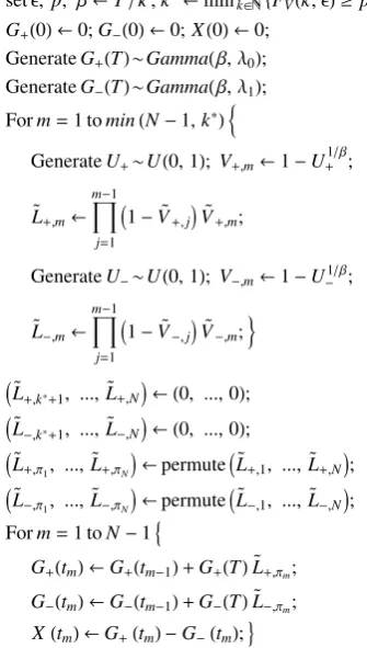
this having an effect on the final estimated price. Proposition 4 (or its alternatives given by (9) and (10)), lead to a refinement of the DirBS method which results in its further substantial speed up as will be shown in the next section. The pseudocode of the proposed Dirichlet Bridge method for sampling of a VG process is given in Figure 1. Note that, in permuting the elements of the random vector

(

˜

L1, . . . ,L˜k∗,0, . . . ,0 )

in order to obtain

(

˜

Lπ

1, . . . ,

˜

Lπ_N )

, there is no need to permute the zero values. Different methods, which could be used in implementing this random permutation, are to be found in Devroye (1986), Chapter 12, and Knuth (1997), p. 145 and p. 148.

4.

Numerical study

set Ε, p; Β ¬TΚ;k*¬minkÎN8FVHk;ΕL³p<; G+H0L¬0;G-H0L¬0;XH0L¬0;

GenerateG+HTL~GammaHΒ,Λ0L; GenerateG-HTL~GammaHΒ,Λ1L; Form=1tominHN-1,k*L:

GenerateU+~UH0, 1L; V+,m¬1-U+

1Β

;

LŽ+,m¬ä j=1

m-1

I1-VŽ+,jMV Ž

+,m;

GenerateU-~UH0, 1L; V-,m¬1-U-1 Β

;

LŽ-,m¬ä j=1

m-1

I1-VŽ-,jMV Ž

-,m;>

ILŽ+,k*₊₁, ...,L Ž

+,NM¬H0, ..., 0L;

ILŽ-,k*₊₁, ...,L Ž

-,NM¬H0, ..., 0L;

ILŽ+,Π1, ...,L Ž

+,ΠNM¬ permuteIL Ž

+,1, ...,L

Ž

+,NM;

ILŽ-,Π1, ...,L Ž

-,ΠNM¬ permuteIL Ž

-,1, ...,L

Ž

-,NM;

Form=1toN-19

G+HtmL¬G+Htm-1L+G+HTLL

Ž

+,Πm;

G-HtmL¬G-Htm-1L+G-HTLL

Ž

-,Πm;

XHtmL¬G+HtmL-G-HtmL;=

Figure 1 Dirichlet Bridge Sampling of a VG Process X(t)with parameters (1, κ, ϑ, σ)at a (finite) sequence of

equidistant time points0 =t0< t1<· · ·< tN=T, (all generated variates are independent).

sampling of VG paths, based on Gamma Sequential Sampling (GSS). The reference set of parame-ters, we use throughout this section,S(0) = 100,ϑ=−0.2859, σ= 0.1927,κ= 0.2505, T= 0.40504,

r= 0.0548, is taken from Hirsa and Madan (2004) and is the one used also by Avramidis and L’Ecuyer (2006).

simulation estimate. As is well known, methods which are characterized by a lower dimension are more RQMC friendly in the sense that generally, they result in smaller errors in the estimate.

The dimension of the problem under the DGBS method is equal to twice the number of time partition points at which values of VG paths are generated, i.e. d= 2N. However, the effective dimension is relatively low, i.e. DGBS is highly QMC friendly, due to the fact that it concentrates the variance on the first few sites of the dyadic partition, used by Avramidis and L’Ecuyer (2006) to produce the gamma bridge points (for a formal definition of effective dimension and further discussions see e.g. Caflisch et al. 1997).

In order to estimate the problem dimension under the DirBS method, we shall use (8) to find the number of increments which need to be generated for each of the two gamma processes,Gi(t;α, λi),

i= 0,1, and therefore, the number of uniforms needed to simulate a trajectory from Gi(t;α, λi),

i= 0,1, (i.e., the r.v.s, ˜Vm in (6)). For the chosen parameter set (κ, ϑ, σ),ϵ= 10−6 andp= 0.99998,

we have solved problem (7) and obtainedk∗=⌈38.7357⌉= 39. One can check that the alternative estimates (9) and (10) give ˆk∗= 39 and ˆk′= 42 forϵ= 10−6 _{and p= 0.99, and for p= 0.99998, (9)}

and (10) give 41 and 55, respectively. Bearing in mind that there are two gamma trajectories per one VG path, each of them requiring 39 uniforms in order to generate the k∗-largest jumps, plus another 39 uniforms to randomly locate them over theN time partition points, plus one uniform used to simulate the terminal value of each gamma process, we arrive atd= 158 (or less ifN <39). The uniform variates, required for the GSS method and in the plain MC versions of DirBS and DGBS, have been generated using the 64-bit universal random number generator of Marsaglia and Tsang (2004). This generator provides numbers with a 1061_{period which pass all the tests developed}

The gamma random variables, required to generate the terminal value of the VG process, have been generated by inversion, based on the Newton algorithm. In the implementation of the DGBS method, the fast generator of symmetrical beta random variables developed by L’Ecuyer and Simard (2006) is employed.

In what follows, the DirBS method is tested and compared with the GSS and the DGBS methods in terms of efficiency. The efficiency ratio is defined as

EA|B=

tBσB2

tAσA2

, (11)

where σ2 _{is the variance of the estimate obtained in time t for the corresponding method. When}

EA_|B>1 we say that methodAis more efficient than (or should be preferred over) methodB and

vice versa if EA_|B<1 (see e.g., Hammersley and Handscomb 1964). Since in our case there is an

estimation bias, in computing the efficiency ratio we have replaced variance by mean square error. For a deeper study of efficiency we refer the interested reader to Glynn and Whitt (1992).

As in Avramidis and L’Ecuyer (2006), we consider the following three options. A floating strike lookback call option with payoff

CT = [

S(T)− inf

0_≤t_≤TS(t) ]

.

A barrier option of the typeup-and-in callwith a payoff

CT = (S(T)−K)

+ 1_{sup

0≤t≤TS(t)>b},

where b > S(0) is the activating barrier and K is the strike price of the European call option underlying the barrier feature. Specifically, we fixK=S(0) = 100 andb= 120. And an Asian option with a payoff

CT = (

1

T

∫ T

0

S(t)dt−K

)+

,

where K is the given strike price. In this case, we consider K=S(0) = 100.

following (3), and an estimate of its variance, we run 100 independent replications (randomizations of the corresponding d-dimensional Sobol’ point sets) with M= 250,000 sample paths.

Both DirBS and DGBS are tested in plain MC environment and also with different number of time points, n≤N, where stratification is applied using a QMC sequence. The results presented here are for the following three cases: n= 0, i.e. the plain MC case; n= 2, when a (randomized) 2-dimensional Sobol’ sequence is used to stratify the terminal values of the two gamma processes,

Gi(tN;α, λi), i= 0,1; and n=nmax, when a (randomized) nmax-dimensional Sobol’ sequence is

used for all (possible) uniforms. This means that, in the case of DGBS,nmax= 2min(N,29), due to

the upper bound of 1111 for the dimension of the Sobol’ sequence used, and in the case of DirBS,

nmax= 158.

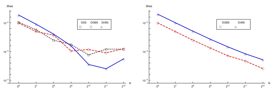
In Figures 2, 3 and 4, the estimated absolute bias for different number of time points, for the lookback, the barrier and the Asian options, respectively is presented in log-log scale. To calculate the bias, we use the estimated exact values, with 95% confidence, of 9.39805±0.00015, 2.1575± 0.0010 and 3.68538±0.000048 for the lookback, the barrier and the Asian options, respectively, obtained by Avramidis and L’Ecuyer (2006), using extrapolation. As can be seen from the left panels of Figures 2, 3 and 4, without stratification the bias of the DirBS method is greater than that for the GSS and the DGBS methods for small number of time points, e.g. N = 26_,27_,28_.

However, for more refined partitions of [0, T], e.g. N = 210_,211_,212_{, DirBS has smaller bias which}

can be explained with the asymptotic nature of the method. In the case of full stratification, the bias decreases with N at the same rate for both DirBS and DGBS, with DirBS behaving more stably, as illustrated in the right panels of Figures 2, 3 and 4.

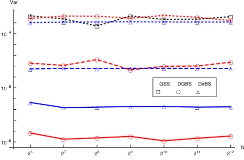
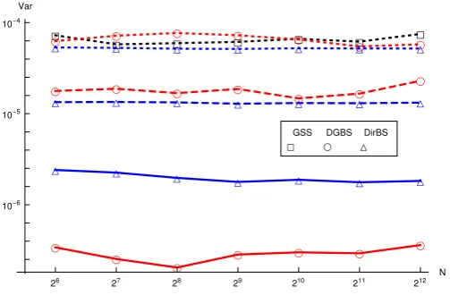
The variance reduction achieved by using the DirBS method compared to the GSS and the DGBS method is illustrated in Figures 5, 6 and 7 in log-log scale for the lookback, the barrier and the Asian options, respectively. We see that stratifying the DirBS and the DGBS method at the terminal time, tN =T, only, leads to similar reduction in the variance for both estimators, with

á á á á á á á ç ç ç ç ç ç ç ó ó ó ó ó ó ó 26 27 28 29 210 211 212

N 10-3

10-2 10-1

 Bias¤

á GSS ç DGBS ó DirBS ç ç ç ç ç ç ç ó ó ó ó ó ó ó

26 27 28 29 210 211 212 N 10-3

10-2 10-1

 Bias¤

ç

DGBS

ó

DirBS

Figure 2 Lookback option example. Estimated absolute bias: n= 0, plain MC (left panel); n=nmax, RQMC

points used for all uniforms (right panel).

á á á á á á á ç ç ç ç ç ç ç ó ó ó ó ó ó ó

26 ₂7 ₂8 ₂9 ₂10 ₂11 ₂12 N 10-3

10-2

 Bias¤

á GSS ç DGBS ó DirBS ç ç ç ç ç ç ç ó ó ó ó ó ó ó

26 ₂7 ₂8 ₂9 ₂10 ₂11 ₂12 N 10-3

10-2

 Bias¤

ç

DGBS

ó

DirBS

Figure 3 Barrier option example. Estimated absolute bias:n= 0, plain MC (left panel);n=nmax, RQMC points

used for all uniforms (right panel).

á á á á á á á ç ç ç ç ç ç ç ó ó ó ó ó ó ó

26 27 28 29 210 211 212

N 10-4

10-3

10-2

 Bias¤

á GSS ç DGBS ó DirBS ç ç ç ç ç ç ç ó ó ó ó ó ó ó

26 27 28 29 210 211 212

N 10-4

10-3

10-2

 Bias¤

ç

DGBS

ó

DirBS

Figure 4 Asian option example. Estimated absolute bias:n= 0, plain MC (left panel);n=nmax, RQMC points

á

á

á

á

á á á

ç ç ç ç ç ç

ç

ó ó ó ó ó ó ó

ç _ç ç

ç ç ç

ç

ó ó ó ó ó ó ó

ç

ç ç ç _ç ç ç

ó

ó ó ó ó ó ó

26 ₂7 ₂8 ₂9 ₂10 ₂11 ₂12

N 10-6

10-5

10-4

Var

á GSS

ç DGBS

ó DirBS

Figure 5 Lookback option example. The variance of the GSS, DGBS and DirBS estimators: n= 0, plain MC

(dotted lines); n= 2, RQMC points used to generate Gi(T, α, λi), i= 0,1 (dashed lines); n=nmax,

RQMC points used for all uniforms (solid lines).

reason for this is because, in DGBS, stratification is applied at a larger number of points than in DirBS. Thus, in the case of DGBS, the values of the two gamma processesGi(t;α, λi), i= 0,1

are stratified at the first nmax= 2min(N,29) time points of the dyadic partition used. Whereas,

for DirBS stratification is applied only in generating Gi(tN;α, λi), i= 0,1, and the sizes and the

positions of the ˆk∗= 39-largest increments of each of the two processesGi(t;α, λi), i= 0,1, which

leads to nmax= 158. However, it has to be noted that using a different low discrepancy sequence,

for example Korobov lattice rules, may lead to different variance reduction factors for the DirBS and DGBS methods. For the DGBS method this has been illustrated in Table 1 of Avramidis et al. (2003).

á á _á á á á á ç ç ç ç ç _ç ç

ó ó ó ó ó ó ó

ç ç

ç _ç

ç

ç ç

ó _ó ó ó ó ó ó

ç

ç

ç ç ç ç

ç

ó _ó

ó ó ó ó ó

26 ₂7 ₂8 ₂9 ₂10 ₂11 ₂12

N 10-5

10-4 Var á GSS ç DGBS ó DirBS

Figure 6 Barrier option example. The variance of the GSS, DGBS and DirBS estimators:n= 0, plain MC (dotted

lines); n= 2, RQMC points used to generate Gi(T, α, λi), i= 0,1 (dashed lines); n=nmax, RQMC

points used for all uniforms (solid lines).

á

á á á á á á

ç ç ç ç ç

ç ç

ó ó ó ó ó ó ó

ç ç _ç ç

ç ç

ç

ó ó ó ó ó ó ó

ç

ç

ç

ç ç ç ç

ó ó _ó

ó ó ó ó

26 27 28 29 210 211 212 N 10-6

10-5

10-4

Var á GSS ç DGBS ó DirBS

Figure 7 Asian option example. The variance of the GSS, DGBS and DirBS estimators:n= 0, plain MC (dotted

lines); n= 2, RQMC points used to generate Gi(T, α, λi), i= 0,1 (dashed lines); n=nmax, RQMC

points used for all uniforms (solid lines).

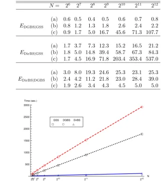
In Figure 8, we give the time for a single run with M= 250,000 sample paths for the lookback option example with full stratification for DirBS and DGBS (the PC used for the calculations has AMD Athlon64FX–55 processor, 2.61GHz and 2.00GB RAM). The computation times for the other two examples are very similar and therefore, are omitted. As can be seen from Figure 8, DirBS is much faster compared to GSS and DGBS. In particular, forN= 26_{, it finishes in 12.27 sec,}

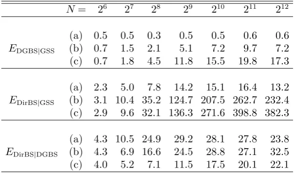
Table 1 Lookback option example. Efficiency gains: (a)n= 0, plain MC; (b)n= 2, RQMC points used to

generateGi(T, α, λi),i= 0,1for DirBS and DGBS; (c)n=nmax, RQMC points used for all uniforms for DirBS

and DGBS.

N= 26 ₂7 ₂8 ₂9 ₂10 ₂11 ₂12

(a) 0.5 0.5 0.4 0.5 0.5 0.5 0.7

EDGBS_|GSS (b) 0.5 0.5 0.6 1.3 2.5 3.6 4.0

(c) 0.5 0.5 0.7 1.4 4.0 14.3 44.1 (a) 1.6 2.5 4.1 8.2 13.6 16.0 19.7

EDirBS|GSS (b) 1.6 2.5 4.2 10.7 30.4 65.3 116.7

(c) 1.6 2.5 4.5 12.1 40.4 133.2 393.0 (a) 3.3 5.4 9.8 15.2 29.2 31.2 28.4

EDirBS|DGBS (b) 3.3 4.9 6.7 8.3 12.0 18.2 29.0

(c) 3.2 4.8 6.5 8.4 10.1 9.3 8.9

Table 2 Barrier option example. Efficiency gains: (a)n= 0, plain MC; (b)n= 2, RQMC points used to generate

Gi(T, α, λi),i= 0,1for DirBS and DGBS; (c)n=nmax, RQMC points used for all uniforms for DirBS and DGBS.

N= 26 ₂7 ₂8 ₂9 ₂10 ₂11 ₂12

(a) 0.5 0.5 0.3 0.5 0.5 0.6 0.6

EDGBS|GSS (b) 0.7 1.5 2.1 5.1 7.2 9.7 7.2

(c) 0.7 1.8 4.5 11.8 15.5 19.8 17.3 (a) 2.3 5.0 7.8 14.2 15.1 16.4 13.2

EDirBS|GSS (b) 3.1 10.4 35.2 124.7 207.5 262.7 232.4

(c) 2.9 9.6 32.1 136.3 271.6 398.8 382.3 (a) 4.3 10.5 24.9 29.2 28.1 27.8 23.8

EDirBS_|DGBS (b) 4.3 6.9 16.6 24.5 28.8 27.1 32.5

(c) 4.0 5.2 7.1 11.5 17.5 20.1 22.1

time is 115.95 sec, and it is 15.41 and 25.28 times faster than GSS and DGBS, respectively. The method becomes more time efficient as the number of time partition points increases. This makes it especially suitable for pricing contingent claims when observations over large (possibly infinite) number of time points are needed.

5.

Comments and conclusions

Table 3 Asian option example. Efficiency gains: (a)n= 0, plain MC; (b)n= 2, RQMC points used to generate

Gi(T, α, λi),i= 0,1for DirBS and DGBS; (c)n=nmax, RQMC points used for all uniforms for DirBS and DGBS.

N = 26 ₂7 ₂8 ₂9 ₂10 ₂11 ₂12

(a) 0.6 0.5 0.4 0.5 0.6 0.7 0.8

EDGBS|GSS (b) 0.8 1.2 1.3 1.8 2.6 2.4 2.2

(c) 0.9 1.7 5.0 16.7 45.6 71.3 107.7 (a) 1.7 3.7 7.3 12.3 15.2 16.5 21.2

EDirBS|GSS (b) 1.8 5.0 14.8 39.4 58.7 67.3 84.3

(c) 1.7 4.5 16.9 71.8 203.4 353.4 537.0 (a) 3.0 8.0 19.3 24.6 25.3 23.1 25.3

EDirBS|DGBS (b) 2.4 4.2 11.2 21.8 23.0 28.4 39.0

(c) 1.9 2.6 3.4 4.3 4.5 5.0 5.0

ááá á

á

á

á

çç ç

ç ç

ç

ç

óó ó ó ó ó ó

26 27

28 29

210

211

212 N 500

1000 1500 2000 2500 3000 TimeHsec.L

á

GSS

ç

DGBS

ó

DirBS

Figure 8 Lookback option example. Computation time for one estimate of the price based on M= 100,000

sample paths.

An interesting insight, which results from our work, is the enlightening interpretation of the generation of the increments of a gamma process at equally spaced time points, given its value at the terminal time, as partitioning of the unit interval into fragments, whose distribution, under the Kingman limit, is GEM(β). Based on this interpretation, we have developed a very efficient method, named DirBS, for simulating trajectories from a VG process, and estimating the price of path-dependent options under the VG model.

A nice feature of the DirBS method is that the related dimension is relatively low and does not increase with the number of time partition points, N. This and the observation that we can simulate ˜Lm by inverting analytically the cdf of ˜Vm (see (6) and Figure 1) makes DirBS very fast

and leads to consistent efficiency gains. The latter is due more to considerable computation time saving (of growing relevance asN increase) rather than to greater variance reduction.

A further direction of research would be to explore the performance of DirBS under alternative choices of low discrepancy sequences (e.g. Korobov lattice rules) and alternative ways of random-izing the QMC (e.g. affine linear scrambling). It would not be surprising to find out that there might be a combination of these alternatives which is more favorable to the performance of DirBS than the chosen Sobol’ sequence and a random shift as the QMC randomization algorithm.

Acknowledgments

The authors would like to thank Dr Laura Ballotta for her valuable contributions to the development of

the C++ code of GSS, DGBS and DirBS methods and for pointing to some relevant references. We also

thank Prof. Pierre L’Ecuyer and Richard Simard for kindly providing us with the C source code of their

Fast Symmetrical Beta generator, and Dr Paul Emms for helping us with various C/C++ implementation

issues. Early versions of this work have been presented at the QMF 2006 Conference, the Maxwell Institute

for Mathematical Sciences, the 14th _{Applied Probability Society of INFORMS Conference. The paper in}

its present form has been presented at the 12th _{International Congress on Insurance: Mathematics and}

Economics and the 3rd _{International Conference on Mathematics in Finance. The authors would like to}

thank the participants of these conferences for useful feedback. The authors would also like to thank the

departmental editor, associate editor, and two anonymous referees for their constructive comments and

References

Ahrens, J.H., U. Dieter. 1974. Computer methods for sampling from gamma, beta, Poisson and binomial

distributions.Computing12 223–246.

Avramidis, A., P. L’Ecuyer. 2006. Efficient Monte Carlo and Quasi-Monte Carlo option pricing under the

variance gamma model.Management Sci.52(30) 1930–1944.

Avramidis, A. N., P. L’Ecuyer, P.A. Tremblay. 2003. Efficient simulation of gamma and variance-gamma

processes.Proc. 2003 Winter Simulation Conf. IEEE Press, Piscataway, NJ, 319–326.

Barrera, J., T. Huillet, C. Paroissin. 2005. Size-biased permutation of Dirichlet partitions and search-cost

distribution.Probability in the Engineering and Informational Sciences1983–97.

Best, D.J. 1983. A note on gamma variate generators with shape parameter less than unity. Computing30

185–188.

Boyle, P., M. Broadie, P. Glasserman. 1997. Monte Carlo methods for security pricing.Journal of Economic

Dynamics and Control21(8-9) 1276–1321.

Bratley, P., B. Fox. 1988. ALGORITHM 659: implementing Sobol’s quasirandom sequence generator.ACM

Transactions on Mathematical Software (TOMS)14(1) 88–100.

Caflisch, R.E., W. Morokoff, A. Owen. 1997. Valuation of mortgage-backed securities using Brownian bridges

to reduce effective dimension.The Journal of Computational Finance1(1) 27–46.

Carr, P., H. Gman, D. Madan, M. Yor. 2002. The fine structure of asset returns:An empirical investigation.

Journal of Business4.

Carr, P., A. Hogan, H. Stein. 2007. Time for a change:The Variance-Gamma model and option pricing.

manuscript.

Chan, T. 1999. Pricing contingent claims on stocks driven by L´evy processes.Annals of Applied Probability

9504–528.

Devroye, L. 1986.Non-uniform Random Variate Generation. Springer.

Daal, E., D. Madan. 2005. An empirical examination of the Variance-Gamma Model for foreign currency

options.Journal of Business 78no 6.

Fiorani, F., E. Luciano. 2006. Credit risk in pure jump structural models.International Center for Economic

Research, Working Paper No. 6.

Fu, M. 2007. Variance-Gamma and Monte Carlo. In Advances in Mathematical Finance. M. C. Fu, R. A.

Jarrow, J.J. Yen, R. J. Elliott eds., Birkh¨auser, 21–35.

Glasserman, P. 2004.Monte Carlo methods in financial engineering. Springer.

Glynn, P.W., W. Whitt. 1992. The asymptotic efficiency of simulation estimators. Operations Research40

505–520.

Hammersley, J.M., D.C. Handscomb. 1964.Monte Carlo Methods.Methuen, London.

Hirsa, A., D. B. Madan. 2004. Pricing American options under variance gamma.The Journal of

Computa-tional Finance7(2) 63–80.

Hirth, U. M. 1997. A Poisson approximation for the Dirichlet law, the Ewens sampling formula and the

Griffiths-Engen-McCloskey law by the Stein-Chen coupling method.Bernoulli3(2) 225–232.

Hurd, T. R. 2007. Credit risk modelling using time-changed Brownian motion.manuscript.

Joe, S., F. Kuo. 2003. Remark on algorithm 659: Implementing Sobol’s quasirandom sequence generator.

ACM Transactions on Mathematical Software (TOMS)29(1) 49–57.

Johnson, N., S. Kotz, N. Balakrishnan. 1997.Discrete multivariate distributions.Wiley.

Kingman, J. F. C. 1975. Random discrete distributions.J. Roy. Statist. Soc. B371–22.

Kingman, J. F. C. 1993.Poisson Processes.Clarendon Press, Oxford.

Knuth, D. 1997. The Art of Computer Programmming, Volume 2:Seminumerical Algorithms, 3-rd edition

Addison Wesley, Oxford.

Kotz, S., N. Balakrishnan, N. Johnson. 2000.Continuous multivariate distributions.2nd ed., Wiley.

L’Ecuyer, P., R. Simard. 2006. Inverting the symmetrical beta distribution.ACM Transactions on

Mathe-matical Software32(4) 509–520.

L’Ecuyer, P., C. Lemieux. 2002. Recent advances in randomized Quasi-Monte Carlo methods. In Modeling

Uncertainty: An Examination of Stochastic Theory, Methods, and Applications.M. Dror, P. L’Ecuyer,

and F. Szidarovszki eds., Kluwer Academic Publishers, 419–474.

Madan, D. B., P. Carr, E. Chang. 1998. The variance gamma process and option pricing.European Finance