On the use of testability measures for dependability assessment

City, University of London Institutional Repository

Citation

:

Bertolino, A. and Strigini, L. (1996). On the use of testability measures for dependability assessment. IEEE Transactions on Software Engineering, 22(2), pp. 97-108. doi: 10.1109/32.485220

This is the unspecified version of the paper.

This version of the publication may differ from the final published

version.

Permanent repository link:

http://openaccess.city.ac.uk/260/

Link to published version

:

http://dx.doi.org/10.1109/32.485220

Copyright and reuse:

City Research Online aims to make research

outputs of City, University of London available to a wider audience.

Copyright and Moral Rights remain with the author(s) and/or copyright

holders. URLs from City Research Online may be freely distributed and

linked to.

On the use of testability measures for

dependability assessment

Antonia Bertolino, Lorenzo Strigini

IEI-CNR, Pisa, Italy

Centre for Software Reliability, City University, London, U.K.

ABSTRACT

Program "testability" is, informally, the probability that a program will fail under test, if it contains at

least one fault. When a dependability assessment has to be derived from the observation of a series of

failure-free test executions (a common need for software subject to "ultra-high reliability"

requirements), measures of testability can - in theory - be used to draw inferences on program

correctness (and hence on its probability of failure in operation). In this paper, we rigorously investigate

the concept of testability and its use in dependability assessment, criticising, and improving on,

previously published results.

We first give a general descriptive model of program execution and testing, on which the different

measures of interest can be defined. We propose a more precise definition of program testability than

that given by other authors, and discuss how to increase testing effectiveness without impairing

program reliability in operation. We then study the mathematics of using testability to estimate, from test

results: i) the probability of program correctness and ii) the probability of failures. To derive the

probability of program correctness, we use a Bayesian inference procedure and argue that this is more

useful than deriving a classical "confidence level". We also show that a high testability is not an

unconditionally desirable property for a program. In particular, for programs complex enough that they

are unlikely to be completely fault-free, increasing testability may produce a program which will be less

trustworthy, even after successful testing.

I. I

NTRODUCTION

This paper studies the relationship between the testability of a program, i.e., informally, the likelihood

that the program reveals its faults during testing, and the trust in failure-free operation that one can

derive for the program from successful testing.

Software testing has an obvious role in finding bugs (in order to remove them), and a less obvious role

in evaluating reliability. No (non-exhaustive) testing procedure can prove the absence of faults in a

program, and the process through which testers reach a belief about the future reliability of the program,

from observing the results of a finite series of tests, is often arbitrary. Specifying how this process

Solving this problem becomes especially difficult in the field of "ultra-high dependability" [18]. There

are applications for which the dependability requirements stated are so high that justifiably claiming,

before operation (as required by safety regulations), that they have been achieved is impossible. The

problem is the paucity of evidence on which the judgement can be based, compared to the extreme

requirements. However, one can hope to raise the levels that can be justifiably claimed, although not in

a dramatic way, by a more accurate interpretation of the evidence available.

For the evaluation of the reliability of software with such high reliability requirements, the normal

scenario is that the program to be evaluated is tested in its final configuration and no fault is found. If a

fault were found, the program would be fixed and testing would restart from scratch: one cannot be

confident that the fix is effective, and, although clearly testing and removing bugs tends on average to

increase reliability, nobody can tell that an individual fix on a certain program will improve its

reliability. So, the only testing session that will lead to the release of the software is one that starts after

the last change to the program and finds no faults. Sooner or later, the testers have to be satisfied that

the software is reliable enough: testing can be stopped and the software can be released.

However, after a long series of successful tests, can one infer that faults are absent, few or

unimportant, as would be desirable, or rather that the testing procedure is ineffective? The normal way

of answering this question is to try and make the testing situation as similar as possible to real operation

[22], and then use statistical inference to infer reliability in operation from the reliability observed in

testing [18], [21], [23]. There are several problems with this approach, not least the difficulty of

choosing a "realistic" test profile (or, worse, a "pessimistic" or "stressful" one).

Another way is to reason directly about the effectiveness of the used testing procedure in finding faults.

Howden and Huang [13], [14] called detectability of a testing method the conditional probability that it

will detect faults, if present, and used this to evaluate a program's trustability, which is a measure of the

confidence in the program being fault-free. Voas and co-authors in [11], [28] introduced a probabilistic

definition of testability , measuring the likelihood of a program to fail, if it is faulty, and suggested that,

by interpreting the results of testing in the light of one's knowledge of the testability of a program, one

could obtain more favourable predictions than allowed by "black-box" based inference alone. These

papers, and more recently [27] and [30], thus propose a method for deriving a confidence in the

program being fault-free using testability estimates. The outline of the reasoning used is: suppose that I

believe that my program, if faulty, is very likely to fail a certain series of tests. Then, if that series is

performed and the program does not fail, it makes sense that the program is likely to be fault-free.

We agree with Voas and co-authors that the concept of testability may shed some light on the question

"How likely is the program to be perfect, if it passed the tests?". However, in this paper we improve on

what we perceive to be serious limitations of the above-quoted papers:

1) their definition of testability does not capture the intuitive notion of "likelihood that testing finds

the faults in a program", and is thus an inappropriate measure, such that using it may lead one to

2) they use a 'classical' inference procedure, producing a 'level of confidence' in the conjecture

that a program is fault-free. This measure is not a sufficient basis for judgement, since programs

may exist that rank equally on this measure, while the degrees to which one can rationally trust

them to be fault-free are clearly different;

3) [11] and [30] claim that a high testability - as they define it - is a desirable property for a

program. This is counter-intuitive: most programs contain bugs, and they are the more useful

the less often these bugs produce failures. It is true that after a series of successful tests a high

testability implies a high probability that the program has no residual faults. But it also implies a

high probability of failure if faults do remain.

We offer therefore the following contributions. In Section II, we give a rigorous conceptual model of

the testing process, with a sound definition of "testability"; in Section III, we discuss how developers

could - through decisions during development and testing - increase the testability of a program (and

hence their ability to assess how reliable it is), without impairing the very reliability that they are trying

to evaluate. In Section IV, we discuss inference from failure-free testing, argue the merits of a Bayesian

approach vs. the "classical" approach of estimating confidence levels and derive the probability of a

program being fault-free, given that its passes testing. Last (Section V), we give a first characterisation

of the conditions under which it is desirable for a software developer to try and improve testability

through changes to programs. Section VI contains our conclusions.

II. G

ENERAL

C

ONCEPTS AND

D

EFINITIONS

A. A Model of Program Execution and Testing

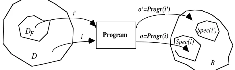
The life of a program is a series of invocations. During each invocation, the program interacts with the

rest of the world, receiving inputs and, as a result, producing outputs. We consider all the information

received by a program during an invocation as one item, called the input for that invocation1_.

The specification of a program unambiguously decides whether the program's output is correct, given

the input that the program received. The specification is a function mapping each input from an input

domain, D, into a set of outputs that are acceptable (given that input), belonging to an output domain,

1 _{More precisely, for a "batch" program, which reads a vector of values once and runs until it terminates producing}

a vector of result values, input and output will designate these two vectors. For a program with memory, "an invocation"

may cover many iterations of reading data, modifying the program's internal state and producing outputs. In this case, we

can call "one invocation" a whole series of read-process-write iterations, an "input" the whole sequence of data read and an

"output" the whole sequence of data produced, possibly including their timing. As an alternative (depending on how the

R. Therefore we say that the program executes correctly on an individual input i, iff the output

produced on that input is compliant with the specification. A program may behave

non-deterministically, i.e., results may differ between executions with identical inputs: we say that the

program is correct on an input i iff it always executes correctly on it. If the program does not execute

correctly on i, we say that a failure took place and that i is a causing input. The set of

failure-causing inputs forms the failure domain D_F, which is a subset of D (see also Fig. 1). A program is

correct (with respect to its specification) iff it is correct on every input; otherwise the program is faulty.

D

D

_{F Program}

R i'

Spec(i)

Spec(i') o=Progr(i)

o'=Progr(i')

[image:5.595.91.500.205.328.2]

i

Fig. 1: Reference model of program execution: this program executes correctly on input i, and

incorrectly on input i'.

Using the definitions in [16], a failure occurs because the program enters an erroneous state. Thus, an

error is a value of [a part of] the system state that can lead to a failure. A fault is the cause (adjudged or

hypothesised) of an error. These definitions make the important distinction between different elements

in the cause-effect chain from "bugs" (faults) to failures. However, one cannot always identify the fault

that caused a failure (there are many ways of changing a program so that a certain input no longer

produces a wrong output), nor what the correct state would be. For our purposes, it will be sufficient to

call "error" any departure of the state of the program from what the programmer had intended it to be

(and call "fault" or "bug" whatever a programmer decides to change, if the change actually eliminates

the problem).

We are interested here in program testing. A test consists of observing the behaviour of the program by

executing it on a certain input. The testing activity requires a controlled environment in which we can

analyse program behaviour. Of course, the outcome of a test depends on many parameters of the

environment, such as the source code, the host on which the program runs, and so on. In the following

discussion, we suppose that all the influencing parameters remain fixed for the whole duration of the

testing exercise.

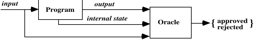
An oracle is any (human or mechanical) agent that decides whether the program behaved correctly on a

given test. The oracle decides about the test outcome by analysing the behaviour of the program against

its specification. In particular, an input/output (I/O) oracle only observes the input and the output of

approved otherwise. If the oracle outputs approved we also say that the test was successful, and

otherwise we say that the test failed.

A more general oracle than the I/O oracle can observe the contents of memory locations and registers in

addition to the program input and output values, and so can decide that a test is rejected as soon as it

detects that the program has entered an erroneous state. It can thus "raise the alarm" even during tests

that produce a correct output, if there are indications that the program is not working as intended by the

programmer. Such general oracles can be obtained by using debuggers or trace analysers as well as by

instrumenting the program with executable assertions for self-checking (a more thorough discussion of

this topic is in Section III-B).

More formally, an oracle implements the following function (see also Fig. 2):

Oracle : D×R ×(Sequences of Values of State Variables) →{approved, rejected}

(where "×" designates the Cartesian product between sets) and is specified to output rejected iff during a test it observes an erroneous value in the program outputs or in the state variables.

Program output

Oracle internal state

{

approved rejected input

[image:6.595.91.503.370.436.2]

}

Fig. 2: The Testing Context

We must consider that the oracle may not always judge correctly. So we introduce the coverage of an

oracle, defined as the probability that it rejects a test (on an input chosen at random from a given

probability distribution of inputs), given that it should reject it, i.e., that the observed -output or

state-variables are erroneous:

Coverage ∆= P(rejected | prob. distribution of inputs, error in observed variables)

The phrase "a probability distribution of the inputs" may require some comment. Of course, testing

requires a mechanism (deterministic or non-deterministic) for selecting inputs. We can usually describe

the series of inputs produced by this mechanism in terms of the probability that each input value (in our

generalised sense, see footnote 1) is chosen, and in most of our modelling we shall refer to a probability

distribution rather than to the specifics of the mechanism actually used.

Most authors assume a perfect oracle (coverage =1). This may be reasonable when considering a run of

comparatively few tests, where a human being examines every result. When many thousands or

millions of tests are required, the oracle must be automated. In most cases, an automated oracle can only

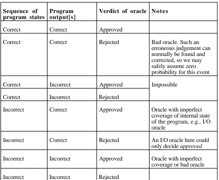
Sequence of program states

Program output[s]

Verdict of oracle N o t e s

Correct Correct Approved

Correct Correct Rejected Bad oracle. Such an

erroneous judgement can normally be found and corrected, so we may safely assume zero probability for this event

Correct Incorrect Approved Impossible

Correct Incorrect Rejected

Incorrect Correct Approved Oracle with imperfect

coverage of internal state of the program, e.g., I/O oracle

Incorrect Correct Rejected An I/O oracle here could

only decide approved

Incorrect Incorrect Approved Oracle with imperfect

coverage or bad oracle

Incorrect Incorrect Rejected

correctness. So incorrect executions may wrongly be accepted, i.e., the coverage is likely to be less

than 1. Considering that real oracles can be imperfect has important consequences. In particular, oracle

coverage affects the reliability level that one can infer from successful testing. [2], for example, explains

how to take account of imperfect oracles for predictions in the form of a one-sided confidence interval

for the program's reliability.

B. Events and Probabilities of Interest

For a probabilistic discussion of testing, we need first to define rigorously the experiment we consider,

its outcomes and the events (sets of outcomes) of interest. We first consider an experiment consisting of

an invocation of the given program, with an input taken from a chosen probability distribution of test

inputs. The outcomes of this experiment are described by the eight rows of Table 1. So the events of

interest may be "the output of the program (or the evolution of its internal state) was correct", or "the

[image:7.595.74.512.320.680.2]

verdict of the oracle was rejected", or any other set of outcomes.

Running T successive tests on the same program is a different experiment, where the space of outcomes

is the Cartesian product of the space of events in Table 1 times itself, T times. If one assigns

probabilities to the eight different outcomes in the single-test experiment, the probabilities of the 8T

outcomes for the T-tests experiment may be derived easily, provided that the tests are statistically

independent (a common hypothesis in testing theory).

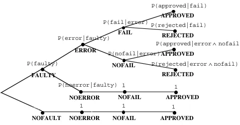
To take into account the knowledge that errors and failures are caused by faults in the program, we now

consider (see Fig. 3) a different experiment associated with the execution of a single test. We consider

that one first, by developing the program, "chooses one program" from a hypothetical population of

"possible" programs which one could develop, and then runs one test on it. Including in the experiment

the step "choice of a program" allows us to consider the two interesting events "the program is faulty"

and "the program has no faults". Fig. 3 is arranged as a tree, with the following meaning. A node in the

tree represents an event, while an arc (N, N’) means that N' ⊆N (N' is a sub-event of N). Nodes are

labelled with the following labels in uppercase characters:

FAULTY: the program is faulty (it has at least one fault).

NOFAULT: the program is correct.

ERROR: on execution, the program enters an erroneous state.

NOERROR: on execution, the program does not enter an erroneous state.

FAIL: on execution, a program failure occurs.

NOFAIL: on execution, no program failure occurs.

APPROVED: on execution, the verdict of the oracle is "approved".

REJECTED: on execution, the verdict of the oracle is "rejected".

A label next to N' indicates what additional property differentiates N' from its parent event N. For

example, if a program is faulty, then the possible sub-events are that either an error happens or not. The

leaf nodes represent the individual outcomes of the experiment. For instance, the top-right node in the

tree represents the event including the one outcome "a program is chosen which is faulty and an error

occurs and the program fails and the verdict of the oracle is approved" and its probability can be

computed by multiplying the probabilities listed in plain text along the path from the root to it. Notice

that all these probabilities are a function not only of the program chosen but of the test input distribution

and of the oracle as well.

To represent the experiment in which two tests are run on the same program, we can extend the tree in

Fig. 3 by attaching, at each of the five leaf nodes of this tree which are descendants of the node

FAULTY, a copy of the whole subtree rooted at FAULTY itself, and by attaching, at the leaf node

descendant from the NOFAULT node, a copy of the subtree rooted at the NOFAULT node itself. These

additional subtrees represent what may happen during the second test. The process can be repeated to

represent all the possible outcomes of running T tests on the same program. We will only be interested

approved for all T tests), the complementary events of these two, and the intersections of these four

events.

In the rest of the paper, we denote by θ the probability that the program will fail on an input drawn at random from a specified probability distribution of the inputs, i.e.:

θ ∆= P(fail | prob. distribution of inputs)

P(nofault)

P(faulty)

FAULTY

NOFAULT NOERROR NOFAIL APPROVED

1 1 ₁

NOERROR NOFAIL APPROVED

P(noerror|faulty) 1 ₁₁

ERROR

NOFAIL

APPROVED APPROVED

REJECTED

REJECTED P(fail|error)

P(fail|error)

FAIL

P(approved|fail)

P(rejected|fail)

P(approved|error nofail)

P(rejected|error nofail)

P(nofail|error)

P(nofail|error)

∧

∧

[image:9.595.47.529.166.417.2]

P(error|faulty)

Fig. 3: Events and Probabilities in the Testing Experiment (we omit impossible events and assume that the oracle will never decide REJECTED on events where NOERROR and NOFAIL hold, as explained in Table 1)

C. Definitions of Testability

We now introduce the notion of testability. We define it based on our model of the testing context,

depicted in Fig. 2. Our definition of testability as a conditional probability2 _{differs in some important}

details from that of Voas and co-authors: for the following discussion, it may be useful to distinguish

between Testab_ABS (our own definition) and Testab_HV (the definition in [11], [27], [28], [30]).

2 _{The word "testability” has also been used without a probabilistic interpretation to capture the intuitive notion of}

how easily a program can be tested, e.g. in [7]. In this sense, it is included for example in the list of quality attributes for

a software product in the standard ISO/IEC 9126 [15]. Alternatively, some authors [4] have defined a notion of

“testability” linked to the effort needed to accomplish the coverage required by various testing methods, e.g., branch

coverage. Even though it is a formal, measurable property of program structure, this notion of testability has no necessary

Definition: Testability (Testab_ABS):

The testability of a program is the probability that a test of the program on an input drawn

from a specified probability distribution of the inputs is rejected, given a specified oracle

and given that the program is faulty.

Testab_ABS ∆= P(rejected | prob. distribution of inputs, oracle, faulty)

Voas and co-authors instead define testability as the conditional probability that the program fails,

without taking into account that failures may go undetected due to an imperfect oracle and that faults can

be revealed (by observing errors) in the absence of failures:

Testab_HV ∆= P(fail | prob. distribution of inputs, faulty)

So, given an input distribution, if we choose a program at random for which we know the value of

Testab_HV and test it once, we have that if the program is faulty, then θ=Testab_HV.

We now briefly discuss the relationship between these two different definitions. We first note that

Testab_HV only depends on the program considered and on the probability distribution of the inputs, while Testab_{ABS depends on the oracle as well. "For a given oracle" and "for a given distribution of the} inputs", we can derive the following formulas (omitting the conditioning on the distribution of inputs

and on the oracle, as we will do in the rest of this paper).

From the definition:

Testab_ABS ∆= P(rejected | faulty)

We can separate, in the formula above, the factors depending on the program under test from those

depending on the oracle, obtaining:

(II.1) Testab_ABS = P(rejected | error) P(error | faulty)=Coverage P(error | faulty)

Since obviously:

(II.2) P(fail) = P(fail | error) P(error | faulty) P(faulty)

the definition of Testab_HV can be written as:

(II.3) Testab_HV ∆= P(fail | faulty)=P(fail | error)P(error | faulty)

Combining Equations II.1 and II.3, we obtain:

(II.4) Testab_ABS =Testab_HV Coverage

We observe that if the oracle is a perfect I/O oracle, then (for a given distribution of the inputs)

Testab_{ABS =TestabHV}.

III. R

ELATIONSHIP BETWEEN TESTABILITY

,

RELIABILITY

,

SOFTWARE DESIGN AND

TEST SET

-

UP

A. The Factors of Testability and Reliability

We now discuss the relationship between testability and other useful properties of a program, especially

reliability, or probability of execution without failure.

The goal of software testing may be (still in the terminology of [16]) fault removal, i.e., reducing the

presence of faults (debug testing), and/or fault forecasting, i.e., estimating the present number of faults

and their future incidence.

- In debug testing, a high testability is clearly desirable in that it reduces the debugging effort.

- In fault forecasting, there are two cases:

(a) testing with the (presumed) operational input distribution to directly measure reliability;

(b) testing with the goal of demonstrating the absence of faults, as normally done in the

industry when attempting a so-called "qualitative" software assessment.

With regard to (b), in [11], [27], [28], [30] Voas and co-authors have proposed a quantitative approach

which uses testability estimates to obtain statements on program correctness. We will discuss this

approach in detail in section IV. These papers also suggest that a high testability is a desirable property

for a program: if a series of tests on a certain program has not revealed failures, then the higher

Testab_HV was for that program, the less likely it is that the program has faults that have gone undetected in testing, that is, the more likely it is that the program is correct. This argument can be discussed from

two points of view: what are its operational implications? and is it true that a high Testab_{HV is}

desirable?

What are its operational implications? Obviously, one could measure Testab_{HV in developed programs}

and use the measured values for dependability evaluation. But, can one obtain higher values of

Testab_{HV through appropriate decisions in the development process? Actually, one can (we shall}

discuss later whether one should). Testab_HV depends on two factors: the structure of the program and the input profile. The structure of the program affects Testab_HV, e.g., through the probability of

executing the possibly faulty modules at each execution of the program, or through the characteristics of

the specified input-output mapping [5], [7]. So, to a limited extent, a developer can try to affect the

value of Testab_HV by choosing certain program structures rather than others (whether biasing the development process this way would be counterproductive would remain to be seen). As for the input

profile, one can, and usually does, vary it during testing to make faults easier to find (i.e., to increase

of little help. To exploit this fact one would have to try and insert only bugs that would be revealed by

some specific test profiles: clearly not a realistic proposition.

Having thus discussed within which limits one can control the value of Testab_{HV through the} development process, the second question is: is it true that a high Testab_{HV is desirable? We observe} that if a program does contain faults, then Testab_HV indicates the failure probability of the program. If, to build a program which has a high value of Testab_{HV during debugging, we make its operation more} vulnerable to its own internal errors, we are likely to end up with a program which is not robust in

operation. The high value of Testab_HV improves our chances of finding out that the program is faulty, but if we still do not find out, it leaves us with a more dangerous program than if Testab_HV had been lower. On the other hand, a program may be very reliable even if it contains many bugs [1]. For

complex programs, this seems to be the norm. Defective code exists, but it is seldom executed;

erroneous internal data are produced, but the errors do not propagate through further processing. One

would like to find and eliminate these bugs, but what ultimately matters is that the program does not fail

in operation, not that it contains no bugs. So, the advice to "design software that has a greater ability to

fail, when faults do exists " [30] can be dangerous.

The confusion arises in part from using Testab_{HV , which is defined as the conditional probability of}

failure, as an indication of the ease of detecting faults during testing. Referring to our description of the

testing context in section II, we can point out that testing can reveal faults even when the program does

not fail, by observing the internal state of the program, and this ability is measured by Testab_ABS. If we distinguish the probabilities of events during operation and during testing (using the superscripts "op"

and "debug", respectively), we can write (see Equations II.1 and II.3):

Pop(fail|faulty)

Testab_ABSdebug =

Pop(fail|error)

Coveragedebug

Pop(error|faulty) Pdebug

(error|faulty)

That is, to make the program reasonably reliable (Pop_{(fail | faulty) reasonably low) and yet reasonably}

well-testable ( Testab_ABSdebug reasonably high), since obviously the variables which are under the

developer's control affect both testability and robustness, the developer can try to: i) make the program

more robust (informally, reduce Pop_{(fail | error)); ii) increase Coverage}debug _{by improving the}

algorithm of the oracle or the observability of the internal state of the program, and/or iii) choose the

input distribution used in testing so as to increase Pdebug_{(error|faulty) (this is - re-phrased- the}

fundamental problem of debug testing, choosing an "effective" test strategy). Last, Pop_{(error|faulty)}

seems difficult to control (one can debug more those modules that are executed more often, but has no

guarantee on the error probabilities due to the residual bugs).

We observe that the ratio between the two factors in i) and ii), Pop_{(fail | error) and Coverage}debug_{, is}

equal to the ratio between Testab_HVopand Testab_ABSdebug (see Equation II.4). In other words, we have an

For the sake of completeness, we note that in [29] Voas and Miller point out the importance of

monitoring the internal state of a program during testing, in particular using assertion checking. In that

paper they "artificially" extend the notion of failure in testing to include failure of inserted assertions.

B. Software Design for Testability and Effects of the Test Set-up

Testability ( Testab_ABSdebug) could be improved by attempts at "design for testability", as used for hardware

[20], [31]. Two considerations apply here. One is that design for testability is based on assumed "fault

models". If one can prove high detectability of certain categories of faults, the problem remains of

deciding the probabilities of faults not belonging to those categories. A similar problem exists with the

estimation of software testability, on which we will return in Section III-D.

A second observation is that "design for testability" for hardware aims at making a system (e.g., a

chip) easier to diagnose as faulty during test, without raising at the same time its failure probability: this

typically involves improving the observability of the inside of the system (e.g. by additional pins,

scan-in-scan-out paths, etc.). This is a useful indication for software as well: one can put some effort into

observing more of the internal state of the software, rather than trying to make it more likely to fail.

Observing the internal state of a program is easy using debuggers, trace analysers and such common

tools. In addition, run-time checking of assertions, in particular of program invariants, at least during

testing, is recommended practice (e.g., [12], [17], [24]). It is a built-in feature in some languages and

easy to implement with any language. The real difficulty is in choosing what (which variables) to

observe, and specifying which conditions its values must satisfy. A concern with this practice is that if

such checks are then turned off for actual operation (typically by not producing the

corresponding object code), a different program is produced than the one tested. Possible solutions

include: using "safer" languages which make it less likely that faults (e.g., memory overwrites) are

masked by the code of the checks; leaving the checks in place in the operational version (a reasonable

practice in critical applications, unless performance limitations then make the application infeasible);

and, as a most general solution, testing the check-less, operational version back-to-back with the

version that contains the check: any discrepancy in behaviour is an event worthy of closer examination.

When debuggers or trace analysers are used, two practical problems exist: these tools are often built for

interactive use, so that they cannot be used to automatically run batches of large numbers of tests; and

they are often intrusive, e.g., because they depend on inserting additional code in the program under

test, or on interrupting its operation with frequent "traps". So, again, the program under test behaves

differently (with certain tools, it is a different program) from the program in normal operation. The

solution is in either using non-intrusive monitoring, for instance via a logic analyser (a solution which

will only be satisfactory for small programs, where few variables need to be monitored), or, as above,

leaving the monitoring software in place during normal operation. The most remarkable example of this

second approach - software design with a self-checking capability- is provided by software fault

tolerance, defensive programming and such (including, e.g., executable assertions with exception

audit programs), which improve both testability and robustness, and thus reliability. With N-version

programming [3], [19], for instance, if a program is built as a combination of three versions derived

from the same functional specifications (and a comparator-voter), any failure of only one of the versions

becomes an internal error of the program, easily detectable under test for the purpose of revealing faults

(high value of Testab_ABS) but not causing a failure of the program, because the voting detects and masks it.

C. A Description of the Debugging Process in Terms of Testability

Testability is a somewhat abstruse concept. For instance, the testability of a fault-free program is the

failure rate that it would exhibit if it were faulty: it describes the characteristics that faults which have not

been detected would have, if they were present. It is thus something which can be estimated, but not

measured with certainty until it is no longer of interest (i.e., after the faults have been found).

It is interesting to describe in terms of testability the different phases of a rational software testing

process aimed at removing faults:

1) we first perform debug testing using a profile expected to yield a high testability (Testab_ABS). 2) By fixing bugs, we change the program and increase its reliability (clearly if fixes are effective

and the faults removed had a non-zero probability of causing failures). Interestingly, we can

expect this debugging process to decrease testability. The faults that might be present are a

mixture of faults with different probabilities of causing failures (under the chosen input profile).

Testability is the average of these probabilities, weighted with each fault's probability of being

actually present in the program. By debugging, we tend to remove first those faults that have

higher probabilities of failure under the input profile we are using. This affects the mix of the

possible faults in the modified program and effectively reduces testability.

3) We then try other test profiles, such as to obtain a high testability again (i.e., profiles with a

high probability of detecting those faults that are more likely to be left in the program). This is

repeated until we are satisfied that the debugging phase may stop (this is often stated in terms of

a specified stopping rule being satisfied). An example of this kind of approach is the "constant

confidence failure-rate" approach in [13]: the input space is partitioned into regions with

different estimated probabilities of failure, and testing is concentrated on the partition with the

highest probability of failure, which changes as bugs are fixed.

4) We then proceed to testing under the operational profile (we may reasonably fear that some

faults have remained undetected), or to actual operation. In this phase, if faults are still found

and fixed, both a reliability improvement and a decrease in testability (for the operational input

D. Evaluating Testability

An open, fundamental problem is how one can evaluate program testability. [26] describes an

experimental technique based on "seeding" simple faults, affecting individual locations (statements or

fragments thereof) in the source code. However, for complex software, this approach is untrustworthy.

We do not know the characteristics and distribution of "authentic" faults, and the artificially seeded

faults can thus cause a wrong estimate of testability measures.

In general, estimating testability requires some knowledge (or assumptions) about the population of

faults and the effect of input distributions. Statistics about failure rates associated with individual faults

could be used directly; statistics of the type of faults observed could be used to drive fault-seeding from

which testability can be estimated. Such knowledge may come reasonably easily, from experience, in

the case of large, complex, buggy software where large populations of faults have been observed; but

for the small, simple, extremely good software products for which it makes sense to expect a high

confidence of freedom from faults, it seems arduous to imagine the behaviour of the population of faults

which might be there and have never been observed. Considerations on the class of program under

evaluation also help. For small procedures, it makes sense to believe that the faults that can be seeded

artificially (typically, simple alterations in one or few statements at a time) are representative of "real"

faults. In this case, the realism of fault-seeding could be enhanced by comparison with real observed

faults, or by trying to pre-filter those seeded faults which would be too obvious to a programmer. In

large, mature software systems, on the other hand, many failures are due to subtle faults, like

mismatches between module interfaces, or a module interfering with the state of another one, which

seem difficult to imitate in a statistically significant manner. Faults may also mask one another, so that

two programming errors, each of which would, by itself, produce failures with high probability, when

both present produce failures with a quite smaller probability: so, seeding individual faults would not

be sufficient.

Other considerations on the structure of the software and its platform are also relevant. For instance,

uninitialised variables make the occurrence of a failure dependent on the whole state of the machine,

thus effectively multiplying the size of the input space and making it possible to have faults with much

smaller failure probabilities: a compiler which prevents the use of uninitialised variables, or, even better,

an architecture which detects it (by defining a "no number" value for the contents of a memory

locations), would thus improve the chance of estimating useful lower bounds on testability. At least for

small programs, reasoning on the program structure, and how it affects the propagation of errors to the

variables checked by an oracle, could help, but it seems that such reasoning would have to be ad-hoc

IV. I

NFERENCE

F

ROM

S

UCCESSFUL

T

ESTING

A. Probability of Failure vs. Probability of Perfection

We now go back to the critical question in the assessment of software for ultra-high reliability: what

exactly can be inferred about the reliability of a software product from tests that reveal no faults? A way

of stating the problem describes testing as a series of independent trials with constant probability of failure (Bernoulli trials). Then, given that the probability of passing one test is (1-θ ), the probability of passing T tests is simply:

(IV.1) P(Tsuccessful tests)=(1-θ )T

On this basis, two different inference procedures are possible, "classical" (see, e.g., [23]) and Bayesian

(e.g., [18], [21]). The differences between the two approaches are discussed later in Section IV-C.

There are difficulties with both inference procedures, including the fact that the estimation of reliability

depends on how closely the input distribution used during testing approximates the operational

distribution in the environment of interest, which is difficult to state [9]. Hamlet suggested [8] [10] that,

rather than trying to estimate the reliability of the software (especially when "ultra-high reliability" is

sought), one may try to estimate the probability that the software is perfect. In any given run, the

probability of failure is obviously less than the probability that the software contains at least a fault (in

fact, faulty software does not usually fail at every execution!).

Attempting to predict absence of faults is of course aiming higher than attempting just to predict an

acceptable probability of failure. Its advantages are:

i) (perhaps obviously) knowledge can be brought to bear that is not otherwise used when

predicting failure rates, that is, the knowledge that without faults no failure is possible;

ii) the testing profile does not need to reproduce an operational distribution, which is difficult, and

it can be chosen so as to best detect faults (i.e., so as to have a high testability), which improves

the confidence that the software that passed all tests is correct ;

iii) if we knew (an upper bound on) the probability that our software is faulty, this would be an

upper bound on the probability of it ever failing. If instead we knew an upper bound of its probability of failure per execution, θ, the probability of its failing over T executions would be bounded by 1-(1-θ)T_{, which tends to 1 as T increases. So, for critical software that must never}

fail over a long period of operation, minuscule values of the probability of failure per execution

would be required to give an acceptable probability that the software will indeed never fail. If,

for instance, we want a 99% probability that a program will never fail over 10 years of operation

at 20 invocations per second, a 99% probability of it being perfect suffices, while the probability

of failure per demand would need to be less than a minuscule 10-11 (with statistical

independence among failures at successive executions, a pessimistic assumption but one for

B. Confidence Level for the Software Being Fault-free

Voas and co-authors [11] [28] proposed a classical "statistical confidence" measure, as follows.

Assume that one has determined a lower bound, h, on the testability (Testab_HV) of a certain program (for a certain distribution of inputs). If one now observes a series of T failure-free tests (on inputs

independently chosen from the appropriate input distribution), the "confidence" in the program being

fault-free is:

(IV.2) 1− (1 - h)T

This can be briefly explained as follows (the explanation in [11] and [28] is different from the

following). How probable is it that the program would pass T tests, if it were really faulty? We said

that, if the program is faulty, its failure rate must be at least h. Then, clearly, its probability of not failing in T tests (see Eq. IV.1) would be less than an upper bound α = (1 - h)T. An upper-bound result like this is normally stated as "there is a confidence (1-α)" that the program is perfect, on the basis of its passing T tests (and of our trust in the lower-bound estimate h for its testability).

More recently, [27] and [30] re-derived this result, with a corrective factor which takes into account the

effects of possible errors in evaluating h as a lower bound on testability.

C. Bayesian Inference and Probabilities vs. Classical Inference and Confidence Levels

The confidence level derived above is a useful measure. For instance, as we increase the number T of

tests, it grows, as does the probability that this particular program is indeed fault-free. However, it

should not be confused with this probability (a confusion which also appears in [11] and [28]). To

understand why, imagine we apply this method to a large number of programs, say, 10,000 programs, all such that our value for α is 0.05, that is, "we have a 95% confidence" that they are perfect. Suppose now that 200 of the 10,000 programs are indeed perfect, and will thus pass the T tests. Of the 9,800

faulty programs, approximately 0.05*9,800=490 will also pass the T tests (more precisely, 490 is the

expected value of the number of programs that will pass the test). If we now consider one program at

random among those that passed the test, the probability that it is fault-free is 200/(200+490)=0.29, not

0.95! So, in this problem, the probability that a program is fault-free, given that it passed T tests, is a

function not only of the "confidence level", characteristic of the test procedure, but also of the

probability that the program was perfect in the first place. Deriving the probability of an event (of the

software being fault-free, in this case) thus requires more information than deriving a confidence level,

but offers important advantages. Given the probabilities of certain events, we can combine them to

derive the probabilities of other events (obtained via set operations intersection, union, complement

-on the events with known probabilities), using a well-known calculus, for instance in the probabilistic

safety assessment of a system. The example above shows how using a confidence level as if it were a

The general formulation of the reasoning procedure given in the example above is Bayesian calculus. In

the Bayesian interpretation, a probability is seen as describing the strength of the belief which a subject

can justifiably hold that a certain event will take place. The subject, upon observing the outcome of an

"experiment" (i.e., the collection of data), updates the belief held before the experiment ("prior

probability") producing a "posterior" probability. In the above example, the prior probability that a

program is perfect was "200 in 10,000" (derived in this case from a knowledge of the proportion of

programs that are perfect). In general, deriving a prior probability for a single event is the difficult part

of Bayesian inference. To estimate the probability that a program is fault-free, one could derive a prior

belief from previous experience with comparable software products and from the static verification

procedures applied on the product to be evaluated (e.g., formal proofs, inspections), in the light of

previous experience with their effectiveness. The use of Bayesian analysis is still opposed by some

scholars, especially because of the need for a "prior belief". However, we think that the example above

is a convincing argument for its use in our case. For another argument, let us imagine that we are testing

two programs, one written by notorious incompetents and one by the best company in the field. After a

few successful tests, the confidence levels for the perfection of the two programs would be the same:

they would certainly not measure one's rationally based trust in the two programs.

D. Bayesian Inference from Failure-free Testing Considering Testability

We now apply the Bayesian approach to our problem. We suppose again that we know the testability of

our program, and that our prior belief in the perfection of our program is P_p. After observing no failures

or errors during testing, our posterior probability (i.e., our updated belief) of the software being correct

is:

(IV.3) P(nofault | T successful tests) =

= P(T successful tests|nofault)P(nofault)

P(T successful tests|nofault)P(nofault)+P(T successful tests|faulty)P(faulty) =

= 1* Pp

1* P_p +P(T successful tests|faulty)(1−P_p) =

P_p

P_p+(1−Testab_ABS)T(1−P_p)

where we have used:

P(T successful tests | faulty) = (1−Testab_ABS)T

from the definition of Testab_ABS.

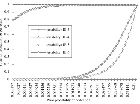
This analysis shows the importance of both the estimated testability and the prior belief in the perfection

of the software in shaping the posterior belief. This effect is shown in Fig. 4, for a fixed number of

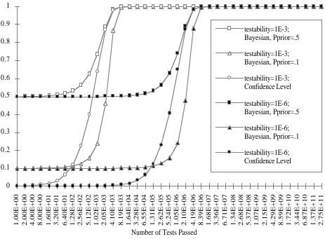
Fig. 5, instead, shows how the posterior probability of the software being fault-free improves with the

number of tests passed. To allow a comparison, the figure includes two curves of confidence levels as

well (for different values of testability). Clearly, these curves are independent of the prior probability

that the software is fault-free3_.

V. I

NFERENCE

A

BOUT

P

ROBABILITY OF

F

AILURE

: W

HEN IS A

H

IGH

V

ALUE OF

T

ESTABILITY

D

ESIRABLE

?

We may now ask ourselves what are the consequences of the above results on our estimate of the

probability of failure for a software product. We do this by considering the same simplified scenario

considered in [11] and [28]: testing with a perfect I/O oracle and under the same input distribution used

in actual operation. We recall that when using a perfect I/O oracle Testab_{ABS =TestabHV} (see Sec. II-C). Since Testab_HV was defined as the probability of failure on an invocation, conditional on the program being faulty, we can write, if we choose a program and then test it once:

θ =Testab_HV* P(faulty)

Given the assumption that we know the value of Testab_HV for the program under test, we can use this expression to update our estimate of θ as we update our estimate of P(nofault), or, accordingly, of P(faulty)=1-P(nofault). Before testing, we have:

θ =TestabHV* (1−Pp)

After the series of T successful tests, we can substitute for Pp the posterior probability of correctness

from Equation IV.3 (in which we have substituted Testab_HV for Testab_{ABS ) obtaining:}

(V.1) θ =Testab_HV* (1−P(no fault |T successful tests)) =

= TestabHV* (1−TestabHV)T(1−Pp)

P_p+(1−Testab_HV)T(1−P_p)

3 _{To underscore again that the confidence level is not a sufficient basis for decisions (e.g. for ranking different programs)}

one can try and quantify the error that using it as a probability would cause. Whenever the prior probability of perfection is

less than 50 % (a reasonable belief for the vast majority of software), using the confidence level as if it were a probability

would increase one's belief, as successful tests accumulate, more than is warranted (by Bayes' rule): after a certain number

of successful tests, the estimate would become too optimistic. As T tends to infinity, the confidence level tends to the

posterior probability for an observer whose prior probability is 50 %. If the testability is of the order of less than 0.1, any

time that Pp < testability, i.e., the prior belief that the software is fault-free is lower than the estimated probability that a

single test would reveal the presence of faults, the confidence level is always an over-optimistic estimate for the posterior probability. For instance, if the prior probability of perfection is 0.1, using the confidence level becomes overoptimistic

Posterior probability of perfection vs prior,

for different values of testability,

after 100,000 tests passed

Prior probability of perfection

Posterior probability of perfection

0 0.1 0.2 0.3 0.4 0.5 0.6 0.7 0.8 0.9 1

0.000177 0.00027 0.000411 0.000627 0.000955 0.001456 0.002219 0.003381 0.005154 0.007855 0.011973 0.018248 0.027813 0.042391 0.064611 0.098477 0.150095 0.228768 0.348678 0.531441

0.81

testability=1E-3

testability=1E-4

testability=1E-5

[image:20.595.71.529.152.494.2]

testability=1E-6

Fig. 4: Posterior probability of a program being fault-free, after passing 100,000 tests, as a

function of the prior probability, for different values of testability

Equation V.1 gives the expected probability of failure per execution, for a program which has passed T

tests and which we trusted correct with probability Pp. We shall now use this expression to answer

more precisely the question posed in Section III-A, i.e., whether it is right for a software developer to

Estimated probability of perfection vs. number of tests passed

Number of Tests Passed 0

0.1 0.2 0.3 0.4 0.5 0.6 0.7 0.8 0.9 1

1.00E+00 2.00E+00 4.00E+00 8.00E+00 1.60E+01 3.20E+01 6.40E+01 1.28E+02 2.56E+02 5.12E+02 1.02E+03 2.05E+03 4.10E+03 8.19E+03 1.64E+04 3.28E+04 6.55E+04 1.31E+05 2.62E+05 5.24E+05 1.05E+06 2.10E+06 4.19E+06 8.39E+06 1.68E+07 3.36E+07 6.71E+07 1.34E+08 2.68E+08 5.37E+08 1.07E+09 2.15E+09 4.29E+09 8.59E+09 1.72E+10 3.44E+10 6.87E+10 1.37E+11 2.75E+11 testability=1E-3; Bayesian, Pprior=.5

testability=1E-3; Bayesian, Pprior=.1

testability=1E-3; Confidence Level

testability=1E-6; Bayesian, Pprior=.5

testability=1E-6; Bayesian, Pprior=.1

[image:21.595.64.527.121.462.2]

testability=1E-6; Confidence Level

Fig. 5 The number of tests (x axis) is shown on a logarithmic scale. The curves starting at 0.1

and 0.5 represent Bayesian inference from a prior belief of 0.1 and 0.5, respectively. The curves starting near 0 represent confidence levels, included here by way of comparison. The curves "bunch up", when approaching their asymptotes, in groups with the same value of testability.

As discussed before, a higher Testab_HV has both a desirable and an undesirable effect: a higher probability that a program that has passed T tests is fault-free, but also a higher θ (equal to Testab_HV itself) for those programs that pass the tests and still contain faults. The expected value of θ, from equation V.1, is an average between these two subsets of the programs that pass the tests. We study

this average as a rough indication of the balance between the two effects; it would be a figure of merit of actual interest for a developer who were concerned with the average θ among many similar products.

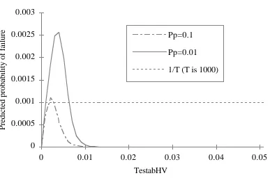
If we study the right-hand expression in Equation V.1, we can notice that it equals 0 when Testab_HV is either 0 or 1, and is positive in between. Fig. 6 shows such curves: all have only one maximum, for a

other hand, for a product which is believed to have a testability lower than this value, only a very large increase in Testab_HV would decrease the estimate of θ. So, the answer to our question is: for testability below t_max(T, P_p), the negative effect of increasing testability (i.e., reducing the robustness of the

software) offsets, on average, its positive effect (i.e., increasing one's confidence in the absence of

faults). For testability above t_max(T, P_p), the reverse is true. By differentiating the expression in Eq.

V.1 we have been able to obtain the following bounds for t_max(T, P_p):

1

T+1<tmax(T, Pp) < 1 P_p•T+1

In particular, one can notice that to some extent T and P_p are interchangeable: either running more

failure-free tests, or having a higher prior belief in the perfection of the product, will change the curve in

Fig. 6, moving its maximum to the left . So, for any value of Testab_HV, planning a long enough series of tests would bring one into the region where a further increase of Testab_HV yields a lower estimate of failure probability. By way of comparison, the horizontal line in Figure 6 shows a Bayesian estimate of

θ, after the same number of successful tests, based on black-box reasoning only. This, as shown, e.g., in [18, 21], is of the order of 1/T (for large values of T), assuming a plausible form of "prior

ignorance". Hence, with a high enough prior belief in the perfection of the software (where "high

enough" is defined as a function of T), a prediction using testability is always more favourable than one

based on the kind of black-box argument described in [18], [21]. However, a lower prior belief will

make it necessary to obtain a rather high testability (Testab_HV=0.01 means that a fault, if present, can be found with a number of tests of the order of 100) for the testability-based prediction to be an

improvement over the black-box prediction. One way of looking at these curves is to consider that, for instance, for Pp=0.1 and testability of the order of 10-4 or less, the posterior probability that the software is fault-free, after 1000 succesful tests, is still around 0.1: 90% of the programs in this

category are expected to contain faults, practically all of them to pass 1000 tests, and the probability of

failure for those that are faulty to be equal to their testability.

There are two ways to improve these results. One is to test with an input profile that is more likely than

the operational profile to uncover faults. Unfortunately, one does not usually know how to select such

tests, once debugging is over and the software is ready for delivery and believed to be very likely to be

Probability of failure vs. TestabHV,

for different prior probabilities of

perfection (1000 tests)

TestabHV

Predicted probability of failure

0 0.0005 0.001 0.0015 0.002 0.0025 0.003

0 0.01 0.02 0.03 0.04 0.05

Pp=0.1

Pp=0.01

[image:23.595.100.487.137.393.2]

1/T (T is 1000)

Fig. 6: Probability of failure, after passing 1000 tests, as a function of Testab_HV, for different values of the prior probability of perfection.

VI. C

ONCLUSIONS

Testability-based reasoning cannot now, and possibly ever, solve the problem of demonstrating

ultra-high reliability of software. The reason is that there is no trustworthy way of measuring the testability of

the programs concerned. By this we do not mean that testability-based reasoning has no role in the

context of ultra-high dependability. First, such mathematical reasoning may indicate a direction for

improvement even when it cannot quantify the achieved improvement. Second, it can be used to correct

fallacies in intuitive reasoning. An evaluator of critical software is often required to reach conclusions

via informal "engineering judgement" on the disparate evidence available. This process is vulnerable to

known limitations of human mental processes [25]. All ways of making this reasoning explicit and

formal improve the chances of detecting inconsistencies and hidden assumptions. Tests of consistency

and plausibility are the main means available for refuting physical theories (including the theory "this

To achieve these advantages, mathematical reasoning must be consistent and must not neglect factors

that are important in reality. We have argued that a proper measure of testability, taking into account the

details of the testing process, is what we defined Testab_ABS, as opposed to Testab_HV, used in [11], [27], [28] and [30]. Our discussion clarifies the roles of the factors affecting testability and reliability:

the coverage of the testing "oracle"; the robustness of the software (its ability - accidental or

intentionally designed-in - to tolerate internal errors); and the relationship between the execution profile

and the distribution of failure-causing inputs in the input space.

We have then shown a Bayesian procedure for inferring from failure-free testing the probability that a

program is fault-free. This procedure allows one to consider some implications of one's premises that

are left hidden when reasoning in terms of 'confidence levels'. In particular, we have shown how the

counter-intuitive notion that higher testability certainly implies a more trustworthy program is indeed

false. The reasoning in [30] would lead an assessor to believe (erroneously) that between two programs

which passed the same number of tests, the one with the higher Testab_HV is to be preferred. Likewise, it would tell a developer to rank alternative design decisions on the basis of how much they raise the

testability of the resulting product. In reality, high testability is desirable to increase one's chance of

obtaining perfect software, but may characterise very failure-prone software. In particular, raising

testability by raising the failure probability under the operational input profile - the basis of the

reasoning in [30] - is a dangerous proposition. On the contrary, the only design provisions that are

certainly beneficial are those that do not increase this failure probability, while increasing the

probability of detecting faults during testing (our Testab_ABS measure). This supports the case for improving the internal error detection capabilities of the software (by any means, from executable

assertions to multiple-version programming), or for using more refined testing tools.

Last, we have given a mathematical description, under simplifying assumptions, of how increasing

testability may be either desirable or detrimental, depending on the current level of testability, the

assessed probability that the software is fault-free (on the basis of evidence available prior to testing),

and the number of tests planned. With a high number of observed successful tests, and a high prior

belief in the perfection of the software, any practice which increases testability appears to be beneficial;

under different conditions, it seems that only a vast increase in testability (under the operational profile)

will be beneficial.

The approach we have studied (testability measures and Bayesian inference) may be made more useful

by gathering more experimental evidence about the actual failure probabilities for classes of programs

of interest, and possibly about the nature of their residual bugs. Our reasoning for deciding when

increasing testability would be beneficial can be made more precise by studying the probability that the

software satisfies its actual reliability requirements, rather than its expected failure probability; by

removing the assumptions that the testability of a program is known with certainty; and by considering

Acknowledgements

This work was funded in part by the European Commission through project "SHIP", "Assessment of

the Safety of Hazardous Industrial Processes in the Presence of Design Faults", in the framework of the

Environment Programme. The authors wish to acknowledge the useful comments and criticism of their

colleagues in Project SHIP, especially Peter Bishop, Peter Popov, Bev Littlewood, and of the TSE

referees.

R

EFERENCES

[1] E. N. Adams, "Optimizing Preventive Service of Software Products", IBM J. of Research

and Development, Vol. 28, No. 1, pp. 2-14, January 1984

[2] P. E. Amman, S. S. Brilliant and J. Knight, "The Effect of Imperfect Error Detection on

Reliability Assessment via Life Testing", IEEE Transactions on Software Engineering, Vol.

20, No. 2, pp 142-148, February 1994.

[3] A. Avizienis, "The N-Version Approach to Fault-Tolerant Software", IEEE Transactions on

Software Engineering, SE-11, No.12, pp.1491-501, 1985.

[4] R. Bache and M. Müllerburg, "Measures of Testability as a Basis for Quality Assurance",

Software Engineering Journal, Vol. 5, pp. 86-92, March 1990.

[5] P.G. Bishop and F.D. Pullen, "Error Masking: a Source of Failure Dependency in

Multi-Version Programs", Proc. 1st IFIP Working Conference on Dependable Computing for

Critical Applications, Santa Barbara, Springer-Verlag, pp. 53-73, 1989.

[6] A. Bondavalli, S. Chiaradonna, F. Di Giandomenico, L. Strigini, "Dependability Analysis

of Iterative Fault-Tolerant Software Considering Correlation", in B. Randell, J,-C. Laprie,

H. Kopetz, B. Littlewood (Eds.), Predictably Dependable Computing Systems, Esprit

Basic Research Series, Springer 1995, pp. 459-471.

[7] R. S. Freedman, "Testability of Software Components", IEEE Transactions on Software

Engineering, Vol. 17, No. 6, pp. 553-564, June 1991.

[8] R. G. Hamlet, "Probable Correctness Theory", Info. Processing Letters, Vol. 25, No. 1,

pp. 17-25, Apr. 1987.

[9] D. Hamlet, "Are We Testing For True Reliability?", IEEE Software, pp. 21-27, July 1992.

[10] D. Hamlet and R. Taylor, "Partition Testing Does Not Inspire Confidence", IEEE

[11] D. Hamlet and J. Voas, "Faults on Its Sleeve: Amplifying Software Reliability Testing",

1993 Int. Symposium on Software Testing and Analysis (ISSTA), Cambridge,

Massachusetts, June 28-30, 1993, pp. 89-98, in ACM SIGSOFT Software Eng. Notes,

Vol. 18 (3), July 1993.

[12] H. Hecht, "Fault-Tolerant Software", IEEE Transactions on Reliability, Vol. R-28, No. 3,

August 1979, pp. 227-232.

[13] W E. Howden and Y. Huang, "Analysis of Testing Methods Using Failure Rate and

Testability Models", tech. report CSE, Univ. of California at San Diego, 1993.

[14] W E. Howden and Y. Huang,"Software Trustability", Proc. of the 5th Int. Symposium on

Soft. Reliability Engineering, Monterey, CA, Nov. 6-9, 1994, pp.143-151.

[15] ISO/IEC 9126, "Information Technology - Software Product Evaluation - Quality

Characteristics and Guidelines for Their Use", first edition 1991.

[16] J. C. Laprie, (Ed.). Dependability: Basic Concepts and Associated Terminology,

"Dependable Computing and Fault-Tolerant Systems" Series, 5th Vol., 265p. Wien,

Springer-Verlag, 1991.

[17] N. G. Leveson, "Safety Assertions for Process-Control Systems", in Proc. 13th

International Symposium on Fault-Tolerant Computing, Milano, Italy, 1983, pp.232-40.,

1983.

[18] B. Littlewood and L. Strigini, "Validation of Ultra-High Dependability for Software-based

Systems", Communications of the ACM , Vol. 36, No. 11, pp. 69-80, November 1993.

[19] M. R. Lyu (Ed.), Software Fault Tolerance, 'Trends in Software' series, 337p., Wiley,

1995.

[20] C. Maunder, The Board Designer's Guide to Testable Logic Circuit, Addison-Wesley,

1992.

[21] K. W. Miller, L. J. Morell, R. E. Noonan, S. K. Park, D. M. Nicol, B. W. Murrill, and J.

M. Voas, "Estimating the Probability of Failure when Testing Reveals No Failures", IEEE

Transactions on Software Engineering, Vol. 18, No.1, pp 33-44, Jan. 1992.

[22] J. D. Musa, "Operational Profiles in Software-Reliability Engineering", IEEE Software, pp.

14-32, March 1993.

[23] D. L. Parnas, A. J. van Schouwen, and S. P. Kwan, "Evaluation of Safety-Critical

[24] C. Rabejac, "On-Line Software Error Detection by Executable Assertions: From Theory to

Practice", Proc. 14th International Conference on Computer Safety, Reliability and Security

SAFECOMP 95, (Belgirate, Italy), 1995.

[25] L. Strigini, "Engineering Judgement in Reliability And Safety And Its Limits: What Can We

Learn From Research in Psychology?", SHIP project technical report T030, July 1994.

[26] J. M. Voas, "PIE: A Dynamic Failure-Based Technique", IEEE Transactions on Software

Engineering, Vol. 18, pp. 717-727, No. 8, August 1992.

[27] J. M. Voas, C. C. Michael and K. W. Miller, "Confidently Assessing a Zero Probability of

Software Failure", High Integrity Systems, Vol. 1, No. 3, pp. 269-275, 1995.

[28] J. M. Voas and K. W. Miller, "Improving the Software Development Process Using

Testability Research", Proc. of the Third Int. Symposium on Soft. Reliability Engineering,

Oct. 7-10, 1992, pp. 114-121.

[29] J. M. Voas and K. W. Miller, "Putting Assertions in Their Place", Proc. of the 5th Int.

Symposium on Soft. Reliability Engineering, Monterey, CA,Nov. 6-9, 1994, pp.152-157.

[30] J. M. Voas and K. W. Miller, "Software Testability: The New Verification", IEEE

Software, pp. 17-28, May 1995.

[31] T. W. Williams and K. P. Parker, "Design for Testability - A Survey", Proc. of the IEEE,