Analysis of Stability and Convergence of Finite-Difference Methods for a
Reaction-Diffusion problem on a One-Dimensional Growing Domain
by
J.A. Mackenzie* and A. Madzvamuse**
[email protected]
[email protected]
Department of Mathematics *
University of Strathclyde
Livingstone Tower
26 Richmond Street
Glasgow, Scotland G1 1XH
Department of Mathematics **
University of Sussex
Mantell Building
Brighton
England, BN1 9RF
Subject classification: AMS(MOS) 65M06 65M12
Keywords: reaction-diffusion, growing domain, stability, bilogical pattern
Running Head: Reaction-diffusion equations on growing domains.
Mailing address: Dr. J.A. Mackenzie
Department of Mathematics
University of Strathclyde
Livingstone Tower
26 Richmond Street
Glasgow, G1 1XH
Scotland
email: [email protected]
Abstract
1
Introduction
In his seminal paper Turing [24] considered a system of two reacting and diffusing chemicals (which he termed morphogens) and demonstrated the surprising phenomenon of diffusion-driven instability. That is, he showed that it was possible for a spatially uniform steady state, linearly stable in the absence of diffusion, to be driven unstable by the presence of diffusion and evolve to a spatially non-uniform steady state. Turing patterns were first observed by Castets et al [2] in a chloride-ionic-malonic-acid (CIMA) reaction and Ouyang and Swinney [20] were the first to observe Turing instability from a spatially uniform state to a patterned state. Although controversial for many years, recent experimental findings strongly support this as a mechanism for the formation of repeated structures in skin organ formation [18, 22] and zebrafish mesoderm cell fates [23].
Most of the applications of Turing theory have assumed fixed domains. For example, in the context of developmental biology, the tacit assumption is that pattern forming processes occur on a much faster timescale in comparison to domain growth. However, it has been shown that in some cases this is not true and that domain growth and domain shape can play a very important role in pattern formation and selection. For example, Kondo and Asai [9] illustrated the role of domain growth in pattern formation by finding mode doubling in patterns of the angelfish
Pomacanthusas it grows. The juvenilePomacanthushas three vertical stripes; once the fish grows to twice its length, new stripes emerge between the original stripes so that the original wavelength is maintained.
straightfor-ward way [3, 9, 21]. On the other hand, the application of finite difference methods to complicated, irregular, and sometimes continuously growing domains is not trivial. It is well known that finite element methods can be applied easily to complicated domains and continuously changing bound-aries can be handled readily by moving grid finite element methods (MGFEM). Madzvamuseet al
[14, 15, 16] investigated, through a novel application of the MGFEM, the role of domain growth to pattern generation on both regular and irregular domains. Numerical simulations in one dimension show solution behaviours such as mode- and period-doubling, peak insertion and splitting. In two dimensions a variety of bifurcations are observed such as transitions from stripe-to-stripe patterns, spots-to-stripes-to-spots patterns, circular patterns and period doubling of spots-patterns.
interaction problems in haemodynamics [19].
Formaggia and Nobile [7] discuss a number of issues related to the formulation of weak ALE formulations for a model scalar convection-diffusion equation; these include the spatial discretisa-tion by Galerkin finite element methods, and the stability of schemes for the numerical integradiscretisa-tion in time of the resulting semi-discrete approximations. An interesting and unexpected outcome of their analysis is the observation that certain implicit temporal integration schemes are only condi-tionally stable depending on the movement of the computational mesh, whereas the same schemes are unconditionally stable when applied to problems posed on fixed meshes. In an attempt to construct an unconditionally stable second-order time integration method, in [11] an analysis was performed of various time integration schemes for a FD-ALE discretisation of a one-dimensional model convection-diffusion problem. By carefully accounting for the diffusive and anti-diffusive effects of the discretisation of the additional terms in the governing equation, the authors were able to propose an adaptive θ-method time integrator which is unconditionally stable, irrespective of the movement of the mesh and is asymptotically second-order accurate in time if the mesh evolves smoothly. It was recently established that with suitable modifications, the same time integrator can successfully be applied to construct an unconditionally stable second-order time integration scheme for a ALE-FEM discretisation of a two-dimensional convection-diffusion problem [12].
although the overall domain may vary with time due to the movement of the domain boundary. For biological growth problems however, it is natural to assume that diffusion and reactions occur in a medium that is moving according to some growth protocol. We will see that when a domain grows it gives rise to an additional convection-like term which is not divergence free. This addi-tional term has a diluting effect on the growth of the analytical solution but we will see that this qualitative behaviour can often be lost under discretisation.
Despite the recent interest in convection-diffusion problems on moving domains, to our knowl-edge very little analysis has been performed for RDEs on continuously deforming domains, where domain growth occurs through a prescribed growth function or can be modelled from experiments as is the case in biology and bio-medicine [17]. The need for such an analysis is evident from the numerical experiments presented in [14], where it was found that domain growth greatly influenced the selection of symmetric solutions obtained using finite difference discretisations.
The layout of this paper is as follows: In Section 2 we present a model reaction-diffusion equation which has been modified to include domain growth. In this section we also consider conservative and non-conservative reformulations of the governing equation with respect to a time independent reference frame. We also derive an energy estimate for the growth of the solution in the special case of linear reaction kinetics and an exponentially growing domain. In Section 3 we present the finite difference spatial discretisations of the conservative and non-conservative formu-lations. In Section 4 we analyse the stability properties of four fully discrete approximations for the model problem of linear reaction on a uniformly growing domain. Conservative discretisations of a linear reaction-diffusion equation are considered in Section 5, where we also present a novel adaptive θ-method and show it is unconditional stable. We prove convergence of the adaptive
2
Model Problem
Reaction-diffusion systems of the type studied in pattern formation generally exclude cross-diffusion, and are only coupled by the reaction kinetics terms. Therefore, we can consider the behaviour of a single chemical species with a straightforward generalisation to a system of interacting chemicals. Let T >0 and for each t ∈[0, T], Ωt be a bounded domain in IR . We shall use the notation
QT ={(x, t)∈IR2 : x∈Ωt, t∈(0, T)}.
Growth of the domain x∈Ωtwith boundary ∂Ωt generates a flowa(x, t). Application of Reynolds transport theorem to the equation for mass conservation for a chemical C, which diffuses with constant density diffusivity κ, undergoing reaction at rateγf(c), gives (see [3])
∂c ∂t +
∂ ∂x
ac−κ∂c ∂x
+γf(c) = 0, (x, t)∈QT
c=c0(x), x∈Ω0, t= 0
c= 0, x∈∂Ωt, t >0,
(2.1)
wherec(x, t) is the concentration at positionxat timetandc0(x) is a well-defined positive bounded
function. The time-varying domain introduces two new terms to the standard reaction-diffusion equation: acx, the transport of material around the domain and cax, the diluting (concentrating) effect of the local volume increase (decrease).
2.1
Arbitrary Lagrangian-Eulerian (ALE) Transformation
domain Ωt at timet, so that
At: Ωc ∈IR→Ωt ∈IR, x(ξ, t) =At(ξ).
We assume that At is bijective and Ωt =At(Ωc) is bounded. We also assume At and its inverse
A−1
t are sufficiently smooth. For a function g :QT →IR defined on the physical domain, the time derivative with respect to the fixed reference domain is
˙
g ≡ ∂g
∂t
ξ
: QT →IR.
If c: QT →IR is regular enough, then by the chain rule
˙
c= ∂c
∂t
x
+ ˙x ∂c ∂x
x
.
The ALE mapping At generates a velocity ˙x defined as
˙
x(x, t) = ∂x
∂t
ξ (A−1
t (x), t).
Rewriting the governing equation (2.1) with respect to the fixed computational coordinates we have
˙
c−κ ∂c
∂x2 −( ˙x−a)
∂c ∂x +c
∂a
∂x +γf(c) = 0, (x, t)∈QT.
If the mapping onto the computational domain is chosen such that ˙x=a, then the transformation is purely Lagrangian and we arrive at the reaction-diffusion equation
˙
c−κ∂
2c
∂x2 +c
∂a
∂x +γf(c) = 0 (x, t)∈QT. (2.2)
Before we discuss numerical approximations of our model problem we first consider the effect that domain growth has on the behaviour of the solution.
2.2
Basic energy estimate
In this section we derive a basic energy estimate for the growth of the L2 norm of the solution
uniform growth of the domain so that ax > 0 is a constant. Note that ax is constant if and only domain growth is exponential [13]
Theorem 2.1 The solution of (2.2) with ax constant and f(c) =c satisfies the following bound
||c||2L2(Ωt)+ 2κ
Z t
0
e−(ax+2γ)(t−s)
||cx||2L2(Ωs) ds =e
−(ax+2γ)t
||c0||2L2(Ω0). (2.3)
Proof Multiplying (2.2) by c and integrating over Ωt we have
Z
Ω(t)
cc˙dx+κ
Z
Ωt
c2xdx+ (ax+γ)
Z
Ωt
c2dx= 0,
where we have used integration by parts and the boundary conditions oncto simplify the diffusion term. Using Reynolds transport theorem we have
Z
Ωt
cc˙dx =
Z
Ωt 1 2
d dt(c
2) dx
= 1 2 d dt Z Ωt
c2dx−
Z
Ωt
axc2dx
.
Therefore, we arrive at the differential equality
d dt||c||
2
L2(Ωt)+ 2κ||cx||
2
L2(Ωt)+ (ax+ 2γ)||c||
2
L2(Ωt) = 0 and the final result follows from a standard Gr¨onwall argument. 2
From (2.3) we can see that domain growth has a diluting effect on theL2 norm of the solution.
In particular, we can see that, if ax+ 2γ >0, then ||c||L2(Ωt) →0 ast→ ∞. In what follows it will become clear that replicating this qualitative behaviour of numerical approximations is non-trivial.
2.3
Uniform domain growth
The second derivative appearing in (2.2) can be rewritten in terms of the derivatives with respect to computational coordinates and we find that
˙
c−κ cξξ x2
ξ
− xξξ
xξ
cξ
!
To make further headway we will assume that the domain growth is uniform and isotropic so that
x(ξ, t) = ρ(t)ξ, where ρ(0) = 1, ρ(t)>0, ∀t >0, (2.5)
with x ∈ Ωt, ξ ∈ Ωc, and ρ(t) is the growth function. If ˙x = a, then it is easy to show that
ax = ˙ρ(t)/ρ(t) and in this case (2.4) simplifies to
˙
c− κ
ρ2(t)cξξ+axc+γf(c) = 0. (2.6)
The coordinate transformation (2.5) therefore results in a reaction-diffusion equation with a time-dependent diffusion coefficient.
We will also be interested in an alternative conservative formulation
˙ (ρc)−κ
cξ
ρ
ξ
+ργf(c) = 0, (2.7)
which can be obtained by multiplying (2.6) by ρ and using the fact that ax = ˙ρ/ρ. The non-conservative and the non-conservative formulation are equivalent at the continuous level but we will see that their numerical discretisations inherit different stability properties.
3
Moving mesh discretisations
We consider semi-discretisations of (2.6) and (2.7) using second-order central finite difference approximations of the spatial derivatives of c. We will assume that the domain Ωt = [xl(t), xr(t)] is covered by a mesh of N cells with
xl(t) =x0(t)< x1(t)< . . . < xN−1(t)< xN(t) =xr(t).
The moving mesh in physical space is assumed to be the image of a fixed uniform mesh covering the computational domain Ωc = [0,1], via the mapping x(ξ, t), so that
The measure of each physical cell will be denoted by
hj(t) =xj(t)−xj−1(t), j = 1, . . . , N.
When we have uniform growth (2.5) then
hj(t) =ρ(t)∆ξ =
ρ(t)
N , j = 1, . . . , N.
To define the semi-discretisations we will use the notation cn
j to denote the approximation of
c(xn
j, tn) andcn = (c0n, cn1, . . . , cnN−1, c
n
N)T. We will use the forward and backward divided differences
(D+c)j =
cj+1−cj
hj+1
and (D−c)j =
cj −cj−1 hj
.
Using this notation the semi-discretisations of (2.6) and (2.7) take the form
˙
cj = 1 ∆ξ
κ
ρ(D+−D−)c
j
−axcj−γf(cj) (3.1)
and
˙
(ρc)j = 1
∆ξ (κ(D+−D−)c)j−γρf(cj). (3.2)
In the following subsections we consider various temporal discretisations of (3.1) and (3.2) and the stability of the resulting fully discrete schemes. The analysis will be carried out using the following mesh-dependent norms. For the numerical solution we use the L2 norm (noting the homogeneous
boundary conditions)
||c||n =
N−1
X
j=1
hn
j+1+hnj 2
(cj)2
!
1 2
.
Approximations of the derivatives will be measured in the cell-based norm
||v||n =
N
X
j=1
hnj(vj)2
!
1 2
.
4
Stability analysis for linear reaction on an exponentially
growing domain
To get some idea of the effect of the growth of the domain on the stability of fully discrete approximations of the conservative and non-conservative formulations, we initially consider the simplified model problem with κ = 0, f(c) = c, with γ a positive constant. Furthermore, we will assume that we have uniform isotropic exponential growth so x(t) = ξeSt, S > 0, and hence
ρ(t) =eSt and a x =S.
4.1
Backward-Euler applied to conservative formulation
Discretising (3.2) in time using the first-order backward Euler (BE) scheme we get
ρn+1cn+1
j −ρncnj
∆t =−γρ
n+1cn+1
j . (4.1)
Rearranging (4.1) we get
cn+1
j =
ρn
ρn+1(1 +γ∆t)c
n j
= e
−S∆t
(1 +γ∆t)c n
j. (4.2)
It is clear from the above that the scheme is unconditionally stable with respect to the l∞ norm.
Note that the effect of the growth of the domain on the dilution of the solution is capturedexactly by the e−S∆t
factor. However, as expected, the backward Euler treatment of the linear reaction term leads to an underestimation in the decrease in the solution as
1
(1 +γ∆t) > e
−γ∆t .
domain. The analysis above can be extended to consider the behaviour of the numerical solution when measured in the mesh dependent L2 norm. It is straightforward to establish from (4.2) that
||cn+1||n+1 = e −S∆t
2 (1 +γ∆t)||c
n||
n. (4.3)
Again, the scheme is unconditionally stable with respect to this norm.
4.2
Backward-Euler applied to non-conservative formulation
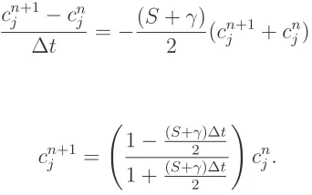
Discretising the non-conservative formulation (3.1) in time using the first-order backward Euler scheme we get
cnj+1−cn j
∆t =−(S+γ)c
n+1
j . (4.4)
Rearranging (4.4) we get
cnj+1 = 1
1 + (S+γ)∆tc
n j.
Therefore, again the scheme is unconditionally stable with respect to the l∞ norm. This time an
error is committed due to the growth of the domain as 1
(1 + S+γ)∆t > e
−(S+γ)∆t .
Furthermore, the non-conservative scheme is less accurate than the conservative BE scheme as 1
1 + (S+γ)∆t >
e−S∆t
(1 +γ∆t) > e
−(S+γ)∆t .
The difference between the performance of both methods will be slight if γ ≫ S for the reasons mentioned above. However, when domain growth is fast compared to the reaction kinetics then
S ≫γ and the non-conservative method should be considerably less accurate than the conservative method. This will be verified by a numerical experiment at the end of this section. For the non-conservative formulation, in terms of the L2 norm we can show that
||cn+1||n+1 = e
S∆t 2
1 + (S+γ)∆t||c
n||
From (4.5) we can deduce that the BE scheme applied to the non-conservative formulation is only conditionally stable if ∆t <∆t∗
, where ∆t∗
is the positive root of the nonlinear algebraic equation
eS∆t2∗ −(S+γ)∆t∗−1 = 0.
This result is somewhat surprising given that the method is fully implicit with respect to the reaction kinetics and is stable with respect to the l∞ norm. This can be explained by the fact that
the L2 norm depends on the measure of Ωt, whereas the l∞ norm does not. Therefore, what is
actually happening is although the nodal value ofcn
j are decreasing asn → ∞, the rate of decrease is not fast enough to ensure that ||cn||n →0.
4.3
Crank-Nicolson applied to conservative formulation
Discretising (3.2) in time using the second-order Crank-Nicolson scheme we get
ρn+1cn+1
j −ρncnj
∆t =−
γ
2(ρ
n+1cn+1
j +ρncnj).
As before we find that
cnj+1 =e−S∆t 1−
γ∆t
2
1 + γ∆2t
!
cnj.
We get perfect dilution from the growth of the domain and the usual second-order Pad´e approxi-mation of the negative exponential decrease from the linear reaction term. Clearly, the scheme is unconditionally stable in l∞. In terms of the L2 norm we easily can show that
||cn+1||n+1 =e−S∆t2 1−
γ∆t
2
1 + γ∆2t
!
||cn||n,
4.4
Crank-Nicolson applied to non-conservative formulation
Discretising (3.1) in time using the second-order Crank-Nicolson scheme we get
cnj+1−cn j ∆t =−
(S+γ) 2 (c
n+1
j +cnj).
As before we find that
cnj+1 = 1−
(S+γ)∆t
2
1 + (S+2γ)∆t
!
cnj.
Again the scheme is unconditionally stable with respect to the l∞ norm and is second-order
accu-rate. Whenγ ≫Swe expect there to be little difference in the quality of the solutions between the conservative and non-conservative CN schemes. The difference will increase however as γ reduces in comparison to S. In terms of the L2 norm we easily can show that
||cn+1||n+1 =eS∆t2
1− (S+2γ)∆t
1 + (S+2γ)∆t
||cn||n.
As with the BE method applied to the non-conservative formulation, we find that the CN method is not unconditionally stable in the L2 norm. In fact, the method is unstable for ∆t >∆t∗, where
∆t∗
is the solution of the nonlinear algebraic equation
eS∆t2∗
1−
S+γ
2
∆t∗
−
S+γ
2
∆t∗
−1 = 0.
Again this result shows that the discretisations of the non-conservative formulation are less stable than their equivalent discretisation of the conservative counterpart.
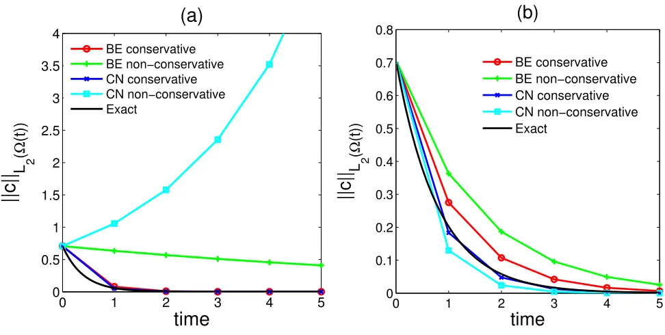
Figure 1 (a) shows the behaviour of||cn||nusing the four methods given above. The calculations
[image:16.595.229.400.135.242.2]L2 norm. We can also see that the non-conservative BE scheme is less accurate than the two
conservative methods. Figure 1 (b) shows the results with γ and ∆t as above, but this time we let
S = 0.5. As expected, there is less discrepancy between the solutions but it is still true that the solutions obtained using the conservative formulations are considerably more accurate than those obtained using the non-conservative form.
The above analysis and results clearly demonstrate that when domain growth is very fast as compared to the reaction times, then non-conservation formulations are unreliable and should not be used. However, for slow growth, such formulations can be used.
0 1 2 3 4 5
0 0.5 1 1.5 2 2.5 3 3.5 4
time
||c||
L 2
(
Ω
(t))
(a)
BE conservative BE non−conservative CN conservative CN non−conservative Exact
0 1 2 3 4 5
0 0.1 0.2 0.3 0.4 0.5 0.6 0.7 0.8
time
||c||
L 2
(
Ω
(t))
(b)
[image:17.595.61.547.297.542.2]BE conservative BE non−conservative CN conservative CN non−conservative Exact
5
Analysis of conservative methods for reaction-diffusion
equation
The analysis in the previous section would appear to suggest that the methods based on the conservative formulation are inherently more stable and more accurate. In this section we will therefore concentrate on these methods and next examine the situation whereκ6= 0, f(c) =cand we will again assume we have uniform growth of the domain.
5.1
Backward Euler
Discretising (3.2) using a backward Euler (BE) temporal discretisation and assumingtn+1−tn = ∆t yields the fully discrete scheme
(ρc)nj+1 = (ρc)nj + ∆t
∆ξ(κ(D+−D−)c)
n+1
j −γ∆t(ρc)nj+1. (5.1)
For this scheme we have the following stability result.
Theorem 5.1 If the scheme (5.1) is applied to the conservative formulation (2.7), then
||cn+1||2
n+1 = (1+2γ∆t) −1
||cn||2
n− ||cn+1−cn||2n−2κ∆t||D+cn+1||2n+1−∆ξ
N−1
X
j=1
[ρn+1−ρn](cnj+1)2
!
.
Proof Multiplying (5.1) by cnj+1 and summing over all interior nodes (since c0 = cN = 0), we have
N−1
X
j=1
ρn+1(1 +γ∆t)(cnj+1)2 = I + II,
where
I = N−1
X
j=1
ρncnjcnj+1,
II = κ∆t ∆ξ
N−1
X
j=1
h
(D+−D−)c
n+1
j
i
Applying the identity
ab= 1 2a
2+ 1
2b
2− 1
2(a−b)
2 (5.2)
to the product cn
jcnj+1 in term I, we have
I = 1 2
N−1
X
j=1
ρn
(cnj)2+ (cnj+1)2−(cnj −cnj+1)2
= 1
2∆ξ ||c
n||2
n+||cn+1||2n+1− ||cn+1−cn||2n
−1
2 N−1
X
j=1
[ρn+1−ρn](cnj+1)2.
For the term II, we have
II = κ∆t ∆ξ
"N−1
X
j=1
cnj+1+1−cnj+1 hnj+1+1
!
cnj+1−
N−2
X
j=0
cnj+1+1−cnj+1 hnj+1+1
!
cnj+1+1
#
= −κ∆t
∆ξ
N−1
X
j=0
cnj+1+1−cnj+1 hnj+1+1
!2
hnj+1+1 =−κ∆t
∆ξ ||D+c
n+1||2
n+1.
Therefore, we have
||cn+1||2
n+1 = (1+2γ∆t) −1
||cn||2
n− ||cn+1−cn||2n−2κ∆t||D+cn+1||2n+1−∆ξ
N−1
X
j=1
[ρn+1−ρn](cnj+1)2
!
,
and this completes the proof. 2
Remark 1 We note here the additional so-called numerical diffusion on the right-hand side of
(5.1), which is represented by the term −||cn+1−cn||2
n. Note that this term would not appear if
the domain were stationary.
Remark 2 This result shows that the discrete L2 norm decreases independently of the time step
as domain growth ensures that ρn+1−ρn>0.
5.2
Forward Euler
It is instructive to consider the forward Euler (FE) scheme for (3.2) which takes the form
(ρc)nj+1 = (ρc)nj + ∆t
∆ξ κ(D+−D−)c
n
j −γ∆t(ρc) n
Multiplying (5.3) by cn
j and following the same analysis as for the BE discretisation, we find that
||cn+1||2
n+1 = (1−2γ∆t)||cn||2n+||cn+1−cn||2n+1−2κ∆t||D+cn||2n−∆ξ N−1
X
j=1
[ρn+1−ρn](cnj)2.
We now have an anti-diffusive term on the right-hand side caused by the mesh movement
||cn+1−cn||2
n+1,
and hence the scheme will be conditionally stable on a moving mesh.
5.3
Mesh-dependent
θ
-method
The question arises if it is possible to combine the BE and FE schemes to create a method that is unconditionally stable and second-order accurate in time. To push through the analysis we consider a weighted combination of a slight variation to the FE and BE schemes given earlier. The new method will involve the modified BE scheme
(ρc)n+1
j = (ρc)nj + ∆t
∆ξκ
cnj+1+1−cnj+1 hθ
j+1
− c
n+1
j −cnj−+11 hθ
j
!
−γ∆t(ρc)n+1
j , (5.4)
where hθ
j =θhnj+1 + (1−θ)hnj. Note that the only difference between (5.1) and (5.4) is the value of hj used in the diffusive terms. Similarly, we use the modified FE scheme
(ρc)nj+1 = (ρc)nj + ∆t ∆ξκ
cn
j+1−cnj
hθ j+1
− c
n
j −cnj−1 hθ
j
!
−γ∆t(ρc)nj. (5.5)
Let us consider a weighted combination of the modified BE and FE schemes of the form θ(5.4) + (1−θ)(5.5), with θ ∈ [0,1]. The stability analysis will be carried out using the mesh-dependent norm
||v||n+θ =
N
X
j=1
(vj)2[θhjn+1+ (1−θ)hnj]
!12
,
which is induced by the inner product
hv,win+θ =
N−1
X
j=1
[θhnj+1+ (1−θ)hnj]vjwj .
Theorem 5.2 The discrete solution obtained using the θ-method with
θ = ρ
n+1
ρn+1+ρn ,
satisfies the following a priori bound
||cn+1||2
n+1 ≤ ||cn||2n−2κ∆t||θD+cn+1+ (1−θ)D+cn||2n+θ, (5.6)
and hence the method is unconditionally stable.
Proof Multiplying throughout the θ-method by θcnj+1+ (1−θ)cn
j we obtain
θ2(BE)cn+1
j +θ(1−θ)(BE)cnj +θ(1−θ)(F E)cnj+1+ (1−θ)2(F E)cnj , (5.7) where BE and F E denote the modified BE and FE schemes. To evaluate PN−1
j=1 (5.7) we need to
first evaluate PN−1
j=1 (BE)cnj and
PN−1
j=1 (F E)c
n+1
j . If we multiply (5.4) by cnj and sum over interior nodes we obtain
N−1
X
j=1
ρn+1(1 +γ∆t)cnj+1cnj = N−1
X
j=1
ρnj(cnj)2+κ∆t
∆ξ
N−1
X
j=1
(
cnj+1+1−cnj+1 hθ
j+1
− c
n+1
j −c n+1
j−1 hθ
j
)
cnj. (5.8)
Replacing the termcnj+1cn
j using (5.2) and substituting forρn+1 in the resulting expression gives (1 + 2γ∆t)||cn+1||2
n+1 = ||cn||2n+||cn+1−cn||2n+1−∆ξ
N−1
X
j=1
[ρn+1−ρn](cnj+1)2
+2κ∆t
∆ξ
N−1
X
j=1
(
cn
j+1−cnj
hθ j+1
−c
n
j −cnj−1 hθ
j
)
cnj. (5.9)
For PN−1
j=1 (F E)c
n+1
j , we have
||cn+1||2
n+1 = (1−2γ∆t)||cn||n2 − ||cn+1−cn||2n−∆ξ N−1
X
j=1
[ρn+1−ρn](cnj)2
+2κ∆t
∆ξ
N−1
X
j=1
(
cn
j+1−cnj
hθ j+1
−c
n
j −cnj−1 hθ
j
)
cnj+1. (5.10)
We now have: PN−1
j=1 (BE)cnj+1 using (5.1) withhnj+1 replaced byhθj in the diffusive term and after multiplying by 2∆ξ gives
(1 + 2γ∆t)||cn+1||2
n+1=||cn||2n− ||cn+1−cn||2n−2κ∆t||D+cn+1||2n+θ−∆ξ N−1
X
j=1
Calculating PN−1
j=1 (F E)cnj using (5.2) with hnj replaced by hθj in the diffusive term after multipli-cation by 2∆ξ gives
||cn+1||2
n+1 = (1−2γ∆t)||cn||2n+||cn+1−cn||2n−2κ∆t||D+cn||2n+θ−∆ξ N−1
X
j=1
[ρn+1−ρn](cnj)2.
Using (5.9), (5.10) and the previous two equations in PN−1
j=1 (5.7), we now have
(1 + 2θγ∆t)||cn+1||2
n+1 = (1−2(1−θ)γ∆t)||cn||2n−θ||cn+1−cn||2n+ (1−θ)||cn+1−cn||2n+1
−2θ2κ∆t||D+cn+1||2n+θ−2(1−θ)2κ∆t||D+cn||2n+θ
−∆ξ
N−1
X
j=1
[ρn+1−ρn] θ(cn+1
j )2 + (1−θ)(cnj)2
+ I,
where
I = 2κθ(1−θ)∆t
N−1
X
j=1
(
cnj+1+1−cnj+1 hθ
j+1
−c
n+1
j −cnj−+11 hθ
j
!
cnj
+ c
n
j+1−cnj
hθ j+1
− c
n
j −cnj−1 hθ
j
!
cnj+1
)
.
On simplification of I, we obtain
I = −4κθ(1−θ)∆t
N−1
X
j=0
cnj+1+1−cnj+1 hθ
j+1
!
cn
j+1−cnj
hθ j+1
!
hθj+1
= −4κθ(1−θ)∆thD+cn+1, D+cnin+θ.
Hence, we have
||cn+1||2
n+1 ≤ ||cn||2n−2κ∆t||θD+cn+1+ (1−θ)D+cn||2n+θ
−θ||cn+1−cn||2
n+ (1−θ)||cn+1−cn||2n+1. (5.11)
We can see from (5.11) that the method will be unconditionally stable and (5.6) will hold if we can ensure that
N−1
X
j=1
A sufficient condition that ensures that this inequality holds is to choose
θ = ρ
n+1
ρn+1+ρn, and this completes the proof. 2
Remark 3 If the domain is growing, then ρn+1 > ρn and hence 1/2 < θ < 1. One might
imagine that the above analysis is unduly pessimistic and that the conservative CN scheme, which
corresponds to the choice of θ = 1/2, is unconditionally stable. However, numerical experiments in Section 7 show that the conservative CN scheme is not unconditionally stable.
Remark 4 If ρ(t) is smooth in the sense that |ρtt| < C for t ∈ [0, T] where C is a bounded
constant, then using Taylor expansions it is relatively simple to show that θ = 1/2 +O(∆t).
6
Convergence result
In this section, we establish a convergence result for the θ-method applied to the conservative formulation. The following lemma establishes a bound on the truncation error.
Lemma 6.1 If the θ-method is applied to the solution of (3.2), then the truncation error satisfies
the bound
Tjn+1 = γ(1−2θ)∆t 2 (ρc˙ ) +
κ(1−2θ)∆t
2ρ
˙
cξξ+
cξξ
ρ
+O(∆t)2+O(N−2
),
where all derivatives are evaluated at (xnj+1/2, tn+1/2).
Proof If the domain growth is uniform, then xξ(t) = ρ(t) and the exact solution satisfies the conservative formulation
˙ (ρc)− κ
The numerical approximation satisfies the equation
ρn+1cn+1
j −ρncnj
∆t = θL
n+1
j cnj+1+ (1−θ)Lnjcnj (6.1)
= θκ
ρn+1
(cnj+1+1−2cjn+1+cnj−+11)
(∆ξ)2 −θρ
n+1γcn+1
j
+ (1−θ)κ
ρn (cn
j+1−2cnj +cnj−1)
(∆ξ)2 −(1−θ)ρ
nγcn
j . (6.2)
We define the truncation error as
Tjn+1 = ρ
n+1c(xn+1
j , tn+1)−ρnc(xnj, tn)
∆t −θL
n+1
j c(xnj+1, tn+1)−(1−θ)Lnjc(xnj, tn) (6.3) = ρ
n+1c(xn+1
j , tn+1)−ρnc(xnj, tn)
∆t −
θκ ρn+1
c(xnj+1+1, tn+1)−2c(xjn+1, tn+1) +c(xnj−+11, tn+1)
(∆ξ)2
+θρn+1γc(xn+1
j , tn+1) + (1−θ)ρnγc(xnj, tn)
− θκ
ρn
c(xn
j+1, tn)−2c(xnj, tn) +c(xnj−1, tn)
(∆ξ)2 . (6.4)
To simplify the truncation error we use the Taylor expansions
ρn=ρn+1/2 −∆t
2 ρ n+1/2
t +
(∆t)2
8 ρ n+1/2
tt +O(∆t)3,
c(xnj, tn) =c(xjn+1/2, tn+1/2)−
∆t
2 c˙
n+1/2 +(∆t)2
8 ¨c
n+1/2 +O(∆t)3,
and similar expansions for ρn+1 and c(xn+1
j , tn+1). Therefore,
ρn+1c(xn+1
j , tn+1)−ρnc(xnj, tn)
∆t =
˙
ρn+1/2c(xn+1/2
j , tn+1/2)
+O(∆t)2 .
It is easy to show that
c(xnj+1+1, tn+1)−2c(xjn+1, tn+1) +c(xnj−+11, tn+1)
(∆ξ)2 =cξξ+
(∆ξ)2
12 cξξξξ+O(∆ξ)
4,
where the derivatives are evaluated at (xn+1
j , tn+1). Hence, overall we have
Tjn+1 = γ(1−2θ)∆t 2 (ρc˙ ) +
κ(1−2θ)∆t
2ρ
˙
cξξ+
cξξ
ρ
+O(∆t)2+O(N−2
),
where all derivatives are evaluated at (xnj+1/2, tn+1/2). 2
Theorem 6.1 If the θ-method is applied to the solution of (3.2), then the global error satisfies the
bound
||En+1||n+1 ≤2∆t
n+1
X
i=1
||T˜i||i ,
where T˜n
j =Tjn/ρn, j = 1, . . . , N −1.
Proof Define the local solution ˆcnj+1 and the local error ˆTjn+1 as follows
ρn+1ˆcn+1
j −ρnc(xnj, tn)
∆t =θL
n+1
j cˆnj+1+ (1−θ)Lnjcnj , (6.5) ˆ
Tjn+1 = ˆcnj+1−c(xnj+1, tn+1). (6.6)
Since
Ejn+1 =cnj+1−cˆnj+1+ ˆcnj+1−c(xnj+1, tn+1),
we have
||En+1||n+1 ≤ ||cn+1−ˆcn+1||n+1+||ˆcn+1−c(xn+1, tn+1)||n+1 . (6.7)
Subtracting (6.5) from (6.1) we obtain
ρn+1[cnj+1−cˆnj+1]−ρn[cnj −ˆcnj] = ∆tθLjn+1(cnj+1−cˆnj+1) + (1−θ)Lnj(cnj −ˆcnj),
since ˆcn
j =c(xnj, tn). Using the stability result (5.6), we have
||cn+1−ˆcn+1||n+1 ≤ ||cn−ˆcn||n=||En||n.
Therefore, (6.7) may be rewritten as
||En+1||n+1 ≤ ||En||n+||cˆn+1−c(xn+1, tn+1)||n+1
= ||En||n+||Tˆn+1||n+1 . (6.8)
From equation (6.6), using (6.3) and (6.5), we have
ρn+1Tˆjn+1 = ρn+1ˆcjn+1−ρn+1c(xnj+1, tn+1)
= −
ρn+1c(xnj+1, tn+1)−ρnc(xnj, tn)
so that
ρn+1Tˆjn+1 =−∆tTjn+1+ ∆t(θLjn+1Tˆjn+1+ (1−θ)LnjTˆjn). (6.9)
Noting that ˆTn
j = 0, we may rewrite (6.9) as
ρn+1Tˆn+1
j −ρnTˆjn
∆t =θL
n+1
j Tˆjn+1+ (1−θ)LnjTˆjn−Tjn+1.
Therefore, except for the truncation error term, we see that ˆTjn+1 satisfies the same equation as the numerical solution. Therefore, proceeding in the same way as the proof of Theorem 5.2, we get
||Tˆn+1||2
n+1 ≤2∆t
N−1
X
j=1
ρn+1Tˆjn+1(Tjn+1/ρn+1)
,
and hence using Cauchy-Schwartz
||Tˆn+1||n+1 ≤2∆t||T˜n+1||n+1.
The equation for the global error (6.8) now takes the form
||En+1||n+1 ≤ ||En||n+ 2∆t||T˜n+1||n+1 ,
and hence we have
||En+1||n+1 ≤2∆t
n+1
X
i=1
||T˜i||i .
2
Remark 5 Theorem 6.1 establishes that the global error is bounded byT˜n
j =Tjn/ρn and hence the
global error converges at the rate O(∆t)2+O(N−2
7
Numerical experiments
7.1
Exponential growth
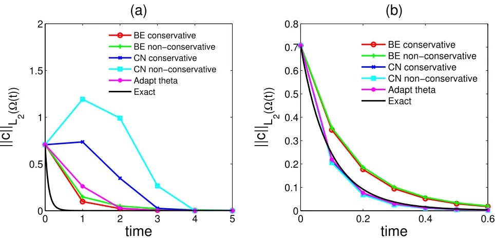
Figure 2 shows the behaviour of ||cn||n using the five methods considered in this paper. The
calculations were performed assuming uniform exponential growth so that ρ(t) = eSt with the parameters γ = 1, κ = 1, S = 0.5 and in (a) ∆t = 1 and in (b) ∆t = 0.1. From Fig. 2(a) we see that when the time step is relatively large there is an unphysical initial increase in the L2 norm
of the solution using both conservative and non-conservative formulations of the Crank-Nicolson scheme. On the other hand, the other three methods all exhibit the correct qualitative behaviour of monotonic decrease in theL2 norm. When we reduce the time step we find that all the solutions
decrease monotonically. As expected however, the accuracy of the backward Euler schemes are poor in comparison with the three second-order methods. Note that the best accuracy is obtained using the adaptive θ-method. When ρ(t) = eSt the parameter θ =eS∆t/(eS∆t+ 1) and hence θ is constant if a uniform time step is used.
7.2
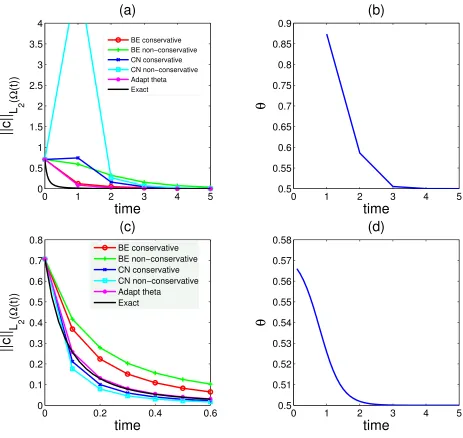
Logistic growth
We next consider the logistic growth function
ρ(t) = e St
1 + L1 (eSt−1),
0 1 2 3 4 5 0
0.5 1 1.5 2
time
||c||
L 2
(
Ω
(t))
(a)
BE conservative BE non−conservative CN conservative CN non−conservative Adapt theta
Exact
0 0.2 0.4 0.6
0 0.1 0.2 0.3 0.4 0.5 0.6 0.7 0.8
time
||c||
L 2
(
Ω
(t))
(b)
BE conservative BE non−conservative CN conservative CN non−conservative Adapt theta
[image:28.595.76.558.66.301.2]Exact
Figure 2: Evolution of ||cn||n for linear reaction-diffusion problem on an exponentially growing
domain: (a) S = 0.5, γ = 1, κ = 1, ∆t = 1, θ = 0.6225 and (b) S = 0.5, γ = 1, κ = 1 and ∆t= 0.1,θ = 0.5125.
0 1 2 3 4 5 0 0.5 1 1.5 2 2.5 3 3.5 4
time
||c||
L 2 ( Ω (t))(a)
BE conservative BE non−conservative CN conservative CN non−conservative Adapt theta Exact0 1 2 3 4 5
0.5 0.55 0.6 0.65 0.7 0.75 0.8 0.85 0.9
time
θ
(b)
0 0.2 0.4 0.6
0 0.1 0.2 0.3 0.4 0.5 0.6 0.7 0.8
time
||c||
L 2 ( Ω (t))(c)
BE conservative BE non−conservative CN conservative CN non−conservative Adapt theta Exact0 1 2 3 4 5
[image:29.595.77.540.66.504.2]0.5 0.51 0.52 0.53 0.54 0.55 0.56 0.57 0.58
time
θ
(d)
Figure 3: Evolution of||cn||nand time integration parameterθfor linear reaction-diffusion problem
on a logistically growing domain with S = 3, γ = 1, κ = 1, L = 10. (a)-(b) ∆t = 1 and (c)-(d) ∆t= 0.1.
8
Conclusions
we found that implicit discretisations of the conservative formulation are more stable in the sense that the L2 norm of the solution decreased independently of the choice of the time step and the
rate of growth of the domain. By contrast, implicit discretisations of the non-conservative refor-mulation were generally only conditionally stable, with the maximal allowable time step being related to the rate of domain growth. The biological implications of our findings are that when the domain grows at a rate much faster than the reaction kinetics, then conservative formulations should be used. In particular, the proposed adaptive θ-method provides computational modellers with an efficient, robust and more accurate scheme which is unconditionally stable as opposed to the conditionally stable forward Euler method which is frequently used in biological simulations of most reaction-convection-diffusion systems.
References
[1] D. Boffi and L. Gastaldi. Stability and geometric conservation laws for ALE formulations.
Comp. Meth. Appl. Mech. Eng., 193:4717–4739, 2004.
[2] V. Castets, E. Dulos, J. Boissonade, and P. De Kepper. Experimental evidence of a sustained standing Turing-type nonequilibrium chemical pattern. Phys. Rev. Lett., 64:2953–2956, 1990.
[3] E.J. Crampin, E.A. Gaffney, and P.K. Maini. Reaction and diffusion on growing domains: Scenarios for robust pattern formation. Bull. Math. Biol., 61:1093–1120, 1999.
[4] E.J. Crampin, W.W. Hackborn, and P.K. Maini. Pattern formation in reaction-diffusion models with non-uniform domain growth. Bull. Math. Biol., 64:746–769, 2002.
[5] J. Donea, S.Giuliani, and J.P. Halleux. An Arbitrary Lagrangian-Eulerian finite element method for transient dynamic fluid-structure interactions. Comp. Meth. Appl. Mech. Engrg., 33:689–723, 1982.
[6] L. Formaggia and F. Nobile. A stability analysis for the arbitrary Lagrangian Eulerian formu-lation with finite elements. East-West Journal of Numerical Mathematics, 7:105–131, 1999.
[7] L. Formaggia and F. Nobile. Stability analysis of second-order time accurate schemes for ALE-FEM. Comp. Meth. Appl. Mech. Eng., 193:4097–4116, 2004.
[8] T.J.R. Hughes, W.K. Liu, and T.K. Zimmermann. Lagrangian-Eulerian finite element for-mulation for incompressible viscous flows. Comp. Meth. Appl. Mech. Engrg., 29:329–349, 1981.
[9] S. Kondo and R. Asai. A reaction-diffusion wave on the skin of the marine angelfish
[10] M. Lesoinne and C. Farhat. Geometric conservation laws for flow problems with moving boundaries and deformable meshes, and their impact on aeroelastic computations. Comput. Methods Appl. Mech. Engrg., 134:71–90., 1996.
[11] J.A. Mackenzie and W.R. Mekwi. An analysis of stability and convergence of a finite differ-ence discretisation of a model parabolic PDE in 1D using a moving mesh. IMA Journal of Numerical Analysis, 27:507–528, 2007.
[12] J.A. Mackenzie and W.R. Mekwi. An unconditionally stable second-order accurate ALE-FEM scheme for two-dimensional convection-diffusion problems. Technical Report 22, Strathclyde University, Mathematics Department, 2007. Submitted for publication.
[13] A. Madzvamuse. Stability analysis of reaction-diffusion systems with constant coefficients on growing domains. Int. J. of Dynamical and Differential Equations, 1(4):250–262, 2008.
[14] A. Madzvamuse and P.K. Maini. Velocity-induced numerical solutions of reaction-diffusion systems on fixed and growing domains. J. Comput. Phys., 225:100–119, 2007.
[15] A. Madzvamuse, P.K. Maini, and A.J. Wathen. A moving grid finite element method applied to a model biological pattern generator. J. Comput. Phys., 190:478–500, 2003.
[16] A. Madzvamuse, P.K. Maini, and A.J. Wathen. A moving grid finite element method for the simulation of pattern generation by Turing models on growing domains. J. Sci. Comput., 24(2):247–262, 2005.
[18] P.K. Maini, R.E. Baker, and C.M. Chong. The Turing model comes of molecular age. Science, 314:1397–1398, 2006.
[19] F. Nobile. Numerical approximation of fluid-structure interaction problems with application to haemodynamics. PhD thesis, Department of Mathematics, ´Ecole Polytechnique F´ed´erale de Lausanne, 2001.
[20] Q. Ouyang and H.L. Swinney. Transition from a uniform state to hexagonal and striped Turing patterns. Nature, 352:610–612, 1991.
[21] R. Plaza, F. Sanchez-Garduno, P. Padilla, R.A. Barrio, and P.K. Maini. The effect of growth and curvature on pattern formation. J. Dyn. Differ. Equ., 16(4):1093–1121, 2004.
[22] S. Sick, S. Reinker, J. Timmer, and T. Schalke. WNT and DKK determine hair follicle spacing through a reaction-diffusion mechanism. Science, 314:1447–1450, 2006.
[23] L. Solnica-Krezel. Vertebrate development: Taming the nodal waves. Curr Biol., 13:R7–9, 2003.