Beyond Intermediates : The Role of Consumption and Commuting in the Construction of Local Input-Output Tables

DEPARTMENT OF ECONOMICS

UNIVERSITY OF STRATHCLYDE

GLASGOW

BEYOND

INTERMEDIATES:

THE

ROLE

OF

CONSUMPTION

AND

COMMUTING

IN

THE

CONSTRUCTION

OF

LOCAL

INPUT

‐

OUTPUT

TABLES

B

Y

KRISTINN

HERMANNSSON

N

O

. 13

‐

05

S

TRATHCLYDE

1

Beyond Intermediates: The Role of Consumption and Commuting in the

Construction of Local Input-Output Tables

Dr Kristinn Hermannsson,

Fraser of Allander Institute, Department of Economics,

University of Strathclyde

[email protected]

Abstract

It is a well-established fact in the literature on simulating Input-Output tables that mechanical methods for estimating intermediate trade lead to biased results where cross-hauling is underestimated and Type-I multipliers are overstated. Repeated findings to this effect have led to a primary emphasis on advocating the accurate estimation of intermediate trade flows. This paper reviews previous research and argues for a qualification of the consensus view: When simulating IO tables, construction approaches need to consider spill-over effects driven by wage and consumption flows. In particular, for the case of metropolitan economies, wage and consumption flows are important if accurate Type-II multipliers are to be obtained. This is demonstrated by constructing an interregional Input-Output table, which captures interdependencies between a city and its commuter belt, nested within the wider regional economy. In addition to identifying

interdependencies caused by interregional intermediate purchases, data on sub-regional household incomes and commuter flows are used to identify

interdependencies from wage payments and household consumption. The construction of the table is varied around a range of assumptions on intermediate trade and household consumption to capture the sensitivity of multipliers.

JEL Codes: C67; R12; R15; R23.

2

1

Introduction

Input-Output (IO) tables offer a variety of applications, such as, for impact studies,

key sector analysis, attribution of greenhouse gas emissions and simply as

multisectoral economic accounts. Furthermore, they are frequently used as inputs

into other modelling approaches, such as Social Accounting Matrices (SAMs) and

Computable General Equilibrium (CGE) models. The best IO tables are produced

based on extensive surveying by national/regional statistical agencies or

international bodies. These are often constructed as part of the process of

compiling national accounts and are resource intensive, well beyond the means of

individual research or consultancy projects. Often an Input-Output table is not

available for a desired geographic unit, and hence has to be simulated. In this case

the academic literature favours using hybrid methods, which are attractive to use

as they require much less primary data collection than full-blown surveying, while

retaining significant accuracy (Lahr, 2003). However, for this the bottleneck is

obtaining actual firm or sector level estimates of intermediate sales and/or

purchases and the resources required are still not trivial. Therefore in practice

researchers and consultants often fall back on mechanical methods, using

secondary data sources to spatially disaggregate existing accounts, using Location

Quotients (LQs).

Several authors (e.g. Harris & Liu 1998) have criticised the use of Location

Quotients to construct local Input-Output. Instead, they typically advocate the use

of hybrid approaches. Despite this clear methodological recommendation

3

data-collection is unfortunately not realistic given typical availability of resources1;

therefore it is worth making further attempts to refine the use of location

quotients.

Whereas previous work has emphasised refining the estimation of intermediate

trade, this paper explores the relative importance of wage and consumption flows

across boundaries, as driven by commuting and shopping trips. To examine this

issue an interregional Input-Output table is constructed for Scotland's largest city

Glasgow, its commuter belt and the rest of the regional economy, based on the

official Scottish IO tables. This is carried out using a location quotient approach,

but augmented with a simple use of secondary data to capture interregional wage

and consumption flows. Sensitivity analysis reveals the relative importance of

specifying interregional wage and consumption flows at the metropolitan level.

This is not surprising given the role of service sectors and extent of commuting in

metropolitan economies in high income countries. The results support the existing

consensus on the importance of accurately specifying intermediate trade, but

suggest that accounting for wage and consumption flows can be equally

important when working with Type-II multipliers.

The paper is structured as follows. The next section introduces the literature on

simulating IO tables. The third section describes the Glasgow metropolitan

economy and its interdependencies with the rest of Scotland. The fourth section

explains the construction of the baseline IO table. In the fifth section a sensitivity

analysis is carried out where the table is re-estimated based on a range of

1 _{With notable exceptions such as the Scottish island economies: Eilean Siar, Shetland and}

4

assumptions about intermediate trade and wage and consumption flows. The

sixth section concludes.

2

Previous research

There are a number of hybrid or partial survey approaches available for estimating

Input-Output tables (see Miller & Blair (2009, Chapter 7) for an overview). These

improve the accuracy of the estimates over purely mechanical approaches by

drawing on actual observations to constrain the results. Typically they proceed in

several steps (Lahr, 1993, p. 278). For example, we could start out with a location

quotient based matrix of intermediate transactions for a local economy. To

improve the accuracy of the estimates it would be possible to survey or conduct

case studies of companies in the most important sectors to determine the total of

intermediate sales (row sum) and purchases (column sum). Numerical approaches

could then be applied to adjust the original matrix to conform to these more

accurate control totals. Or as put more generally by Snickars & Weibull (1977)

information about macro states can be used to inform estimates of micro states.

As summarised by Lahr & de Mesnard (2004) there are a range of techniques

available for reconciling partial observations with estimates. Within the context of

Input-Output tables the RAS Technique is probably the most well-known of these

(see Section 7.4 in Miller & Blair (2009)). As Lahr & de Mesnard (2004) point out

these adjustment algorithms fall into broadly two categories: Scaling algorithms,

of which RAS is one, and maximizing algorithms. Prominent examples of the latter

are entropy maximisation principles (Wilson 1970) or Efficient Information

Adding. Snickars & Weibull (1977) discuss the general principle and demonstrate

its application to several spatial-economic problems. The approach is discussed

5

Snickars (1979) demonstrates its application to estimating interregional trade

within Sweden.

Notable past contributions have acknowledged the problem that at the

metropolitan level local economies are strongly interdependent through

commuting and shopping trips (Hewings et al 2001, Jun 1999, 2004, Madden

1985). Therefore, particular care needs to be taken when the boundaries of the

study area cross functional boundaries (Hewings & Parr, 2007). Madden (1985)

clearly lays out the theory for a multiregional metropolitan input-output model

allowing for commuting and shopping trips. Its use is demonstrated for

Nordrein-Westphalia in Germany, but the author does not elaborate on the data sources

used. Hewings et al (2001) set out a theoretical structure for a 4-region

metropolitan input-output model, which they apply to the Chicago economy. The

database is constructed based on LQs in combination with commuting and

shopping matrices. These models offer a number of advanced features. However,

what data collection they involve is not clear and these have yet to be distilled

into simple approaches, which could readily be implemented in practice, for

example by resource constrained policy makers and consultants.

2.1

Location Quotients

The widespread use of the LQ approach for constructing regional Input-Output

tables is primarily driven by pragmatic concerns. Detailed data are seldom

available at the regional level to implement more accurate methods and collecting

the primary data needed is typically beyond the means of the IO-users. Given this

predicament a typical response is to draw on a published input output table

6

estimate a local sub-section of that table. Implicitly by going down that route the

researcher is accepting some rather bold assumptions. For these Harris & Liu

(1998) refer to Norcliffe (1983, pp. 162-163), which identifies the main

assumptions underlying the use of location quotients to identify the export base

in export base models2.

It is clear that for employment to be used as a proxy for output there must be

identical productivity per employee in each region in each industry so that a

region’s share of national employment accurately represents its share of national

production. Furthermore, for similar reasons, there must be identical

consumption per employee. Perhaps most importantly however, so as not to

underestimate interregional trade, there must be no cross-hauling between

regions of products belonging to the same industrial category. Given that these

assumptions rarely hold, a number of authors have attempted firstly to estimate

empirically the extent to which the breakdown of these assumptions will

influence estimates for IO-accounts and secondly to come up with modifications

of the LQ-approaches that might counter some of the inherent biases.

Various LQ methods have been suggested in the literature (Miller & Blair, 2009,

pp. 349-360). In general LQ approaches adjust the national technical coefficient to

take account of the potential for satisfying input needs locally. A regional

Input-Output coefficient is a function of the location quotient and the national Input

Output coefficient:

2 _{Norcliee identifies 4 main assumptions. However, his fourth assumption is not relevant in}

7

(

)

ij R i RR ij RR

ij

a

LQ

a

a

=

,

Where

a

and

a

2.1.1 Simple location quotient (SLQ)

The simple location quotient for sector i in region R is defined as:

       

= _{N N}

i R R i R i E E E E SLQ

Where E_iR and

E

in region R respectively and E_iN and

E

employment in the nation as a whole.

When the SLQi is greater than one (less than one), it can be inferred that sector i is

more (less) concentrated in region R than in the nation as a whole. Where the

location quotient is less than one the region is perceived to be less able to satisfy

regional demand for its output, and the national coefficients are adjusted

downwards by multiplying them by the location quotient for sector i in region R.

Where the sector is more concentrated in the region than the nation at large

(LQi>1), it is assumed that the regional sector has the same coefficients as the

nation as a whole. Therefore for row i of the regional table:

1

1

≥

<

=

SLQ

SLQ

if

if

a

SLQ

a

a

8

2.1.2 Cross industry location quotient

A criticism of the simple location quotient is that it does not take into account the

relative size of the sectors engaged in intermediate transactions. The argument

goes that if a sector which is relatively small locally is supplying a sector which is

relatively big, this should imply a need for imports to satisfy intermediate

demand, and vice versa. This is addressed with cross industry location quotients

(CILC). The CILQ for sectors i and j can be defined as:

















=

E

E

E

E

SLQ

SLQ

CILQ

Where sector i is assumed to be supplying inputs to sector j. As with the SLQ

national coefficients are not adjusted if ≥ 1 as it is assumed that

intermediate demand can be met within the economy.

2.1.3 Round’s semi-logarithmic Location Quotient (RLQ)

Round (1978, p. 181) surmises that “following the basic notion of the location

quotient, one could reasonably conjecture that the size of trading coefficient may

be ascertained by some function of the relative size of the supplying sector, the

relative size of the purchasing sector, and the overall size of the region relative to

the nation as a whole“. In order to incorporate all three of these measures in a

location quotient, Round (1978) suggested a semilogarithmic quotient, which he

defined as

= / log1 +

2.1.4 Flegg, Webber and Elliot’s Location Quotient (FLQ)

Flegg, Webber and Elliot introduce the FLQ approach (Flegg et al, 1995), which is

subsequently developed in Flegg et al (1997) and Flegg et al (2000). In this

9

region such that =λ, where λ = log1 + E/E , where

0 ≤ # ≤ 1. Then

$%%= _$

' () > 1

$' () < 1

The aim is to reduce national coefficients more for smaller regions, under the

general expectation that smaller regions are more import intensive. The main

difficulty with this method is that it requires an ad hoc assumption about the

parameter δ. Initially, Flegg & Webber (1997) propose that an approximate value

for δ=0.3 ”would seem reasonable” (p. 798). However, subsequently efforts have

been extended to select an appropriate parameter through empirical testing.

2.2

Empirical testing of alternative LQ methods

A number of studies have been undertaken to test the accuracy of hybrid and

non-survey methods. See for example: Schaffer & Chu (1969); Smith & Morrison

(1974); Round (1978); Harrigan et al (1980ab); Willis (1987); Harris & Liu (1998);

Tohmo (2004); Stoeckl (2010); and Flegg & Tohmo (2011). The resulting

consensus is that IO-tables constructed using location quotients produce

multipliers that are systematically biased upwards. These tables tend to

underestimate imports and exports and overestimate local intermediate

transactions. This is primarily due to their failure to acknowledge cross-hauling

(Harris & Liu, 1998). Secondly, when Type-II multipliers are used, an accurate

identification of household consumption and labour income is critical for accurate

multipliers (Lahr 1993, Richardson 1985).

Tohmo (2004) summarises the findings of five studies comparing multipliers

10

Morrison (1974), Harrigan et al (1980b), Flegg & Webber (1996) and Harris & Liu

(1997) in addition to his own analysis. This reveals that it does not seem to make

much difference whether the SLQ, CILC or the RLQ formulas are used. These

methods produce multipliers that are on average biased upwards by 12-25%. An

exception to this is the FLQ formula, which is able to recreate on average4 the

multipliers obtained from a surveyed Input-Output table. However, this depends

on identifying the right adjustment parameter, which is not known ex ante but

has to be deduced from comparison with surveyed tables ex post. Flegg & Tohmo

(2011) discuss this issue in detail and test parameter values by simulating IO

tables for 20 Finnish regions of various sizes.

The academic debate on formulating appropriate location quotients is mostly

concerned with finding the most appropriate method to counter the bias of

overestimating regional multipliers (Flegg et al, 1995, Flegg & Webber, 1997,

2000, Brand 1997). However, McCann & Dewhurst (1998) point out that in some

cases, particularly where strong regional specialization occurs, traditional

LQ-approaches can actually underestimate local multipliers by over-estimating

interregional trade. Flegg & Webber (2000) acknowledge this point in principle

but argue that based on empirical testing this does not seem to be a significant

concern in practice. Furthermore, the upward bias to multipliers derived from

LQ-based IO-tables does not seem to be uniform across regions or sectors. For

example Harris & Liu (1998) point out that this bias is more acute for traded

sectors such as manufacturing than for services.

4 _Flegg et al _{(1995, p.548) point out that even if the systematic errors are removed,}

11

Previous research has primarily focussed on the role of trade. This is certainly

important, but ex ante it can be expected that the smaller the scale of the

economy being examined, the more pertinent the role of wage and consumption

flows across boundaries. For example, Roberts (2005) demonstrates the relative

importance of households consumption in rural economies and Hewings et al

(2001) demonstrate the relative importance of these effects in their IO-table of

the Chicago Metropolitan Economy.

3

Glasgow City-region and the rest of Scotland

This paper focuses on Glasgow, which is the largest city in Scotland, with a

city-region (comprising Glasgow (GLA) and the rest of Strathclyde (RST)) of

approximately 2.1 million inhabitants5. GLA is a separate administrative unit but is

economically interdependent with the RST and the Rest of Scotland (ROS). The

ROS is identified as a residual, to allow the spatial boundaries of the study to

conform to Scotland. The Strathclyde region is Scotland's largest population and

economic centre, containing 41.7% of its population and 41.1% of total

employment. At its centre is the City of Glasgow, which is linked via an extensive

suburban rail network to the rest of the Strathclyde region. Key economic and

social indicators for these areas are given in Table 1.

Table 1 Key social and economic indicators for each IO-region in 2006.

GLA RST ROS SCO

Population 000's 580,690 1,555,374 2,980,836 5,116,900

5 _{This is a wide definition of Glasgow city-region encompassing the whole of the former}

12

% of total 11% 30% 58% 100%

Employment FTEs 313,535 448,296 1,089,529 1,851,360

% of total 17% 24% 59% 100%

Gross Domestic Household Income Per Capita

£ 11,968 12,975 13,319 13,071

% of

average 92% 99% 102% 100%

Within Strathclyde the main focus is on the Glasgow City Council jurisdiction,

which spans an area of 175 km2 and included 581 thousand inhabitants in 2006.

Roughly 313 thousand full time equivalent jobs are found in Glasgow, which is

approximately 17% of total employment in Scotland. This is a much larger share of

Scotland-wide employment than Glasgow’s population share would suggest – to

the extent that (as is illustrated in Table 2) four out of every ten jobs in the city

are taken by in-commuters, primarily originating from other parts of the

Strathclyde region.

The rest of the Strathclyde region (RST) has somewhat different economic

characteristics than Glasgow (GLA). In terms of population it is approximately 3

times the size of Glasgow. However, there are only 1.4 times as many jobs in RST

as there are in GLA. As is evident from Table 2 the lower job density in the RST

region is explained by significant out-commuting to seek employment in Glasgow

(40% of all those working in Glasgow come from the rest of the Strathclyde

region). Furthermore, households in RST bring significant amounts of consumer

13

Table 2 Origins and destinations of people who travel between Scottish

addresses for work/study (headcount/column %). Own calculations, based on

Fleming (2006, Table 16A, pp. 64-65).

Place of work

GLA RST ROS SCO

R

e

si

d

e

n

ce GLA 246,938 59% 46,677 6% 4,743 0% 298,360 11%

RST 167,322 40% 727,112 93% 16,258 1% 910,694 32%

ROS 5,961 1% 6,335 1% 1,613,211 99% 1,625,507 57%

420,221 100% 780,125 100% 1,634,212 100% 2,834,560 100%

4

Construction of the Input-Output table

The Scottish Input-Output tables for 2006 are disaggregated into three

sub-regions. The process is presented schematically on the next page6. The IO-table

has i intermediate sectors, q final demand sectors and p primary (i.e. value added

categories) sectors. The notation is as follows (small bold cases for vectors and

capital bold cases for matrices):

x = i-vector of outputs

Z = i x i - matrix-of intermediate demand

F = i x q - matrix-of final demand

V = p x i– matrix of primary costs

The superscripts indicate the spatial origin and destination of the matrix elements,

with G representing Glasgow, W the rest of the Strathclyde region and S the rest

of Scotland. The order follows the familiar row/column convention for matrix

elements, for example the matrix ZWG contains the elements for the intermediate

demand rows (origin) of the rest of Strathclyde region (W) and the intermediate

expenditure column of Glasgow (G), which is the destination of the expenditures.

6 _{The schematics are based on Oosterhaven & Stelder (2007), which provides an accessible}

14

Figure 1 Single region IO-table for Scotland

For final demand and primary inputs the table is more complicated. The

household consumption category of final demand has a region of origin and a

region of destination. This q1category is represented by the interregional matrices

FGG, FGW, FGS, FWG, FWW, FWS, FSG, FSW and FSS. The q2 final demand categories are not

assigned a spatial origin (from within the interregional IO-accounts), e.g.

government and capital formation (and export) final demand. These matrices are

denoted as FG*, FW*, FS*.

Figure 2 Interregional Input-Output table for three regions (r = 3) ←---i---→ ←----q----→ ← -- i- ---→

Z F _→ ΣΣΣΣ x

← --p --→ V Σ Σ Σ Σ↓ x

←-q2-→

Z

Z

Z

F

F

F

F

Z

Z

Z

F

F

F

F

Z

Z

Z

F

F

F

F

V

V

V

V

V

V

V

V

V

←

-p2

-→

V

V

V

Σ Σ Σ Σ↓

x

→

x

15

The disaggregation process is carried out at the most disaggregated level

permitted by the Scottish IO tables (126 sectors)7 and occurs in 4 stages:

1. Estimate sector gross output totals

2. Estimate technical coefficients (A-matrices) and intermediate

transactions (Z-matrices)

3. Estimate primary inputs

4. Estimate final demands and balance table

Data on employment by sector and NUTS 3 region are obtained from the 2006

Annual Business Inquiry (ABI) using the NOMIS data portal8. The IO sectors in the

Scottish IO-table refer to specific Standard Industrial Classification (SIC) categories

and therefore employment levels from the ABI can be matched to each IO-sector.

4.1

Step 1: Sector gross output totals for GLA-RST-ROS

To derive gross output totals by industrial sector and sub-region employment is

used to disaggregate output levels from the Scottish input output table:













=

N i

R i N i R i

E

E

x

x

Where x_iR refers to output of sector i in region R and x_iN refers to output of

sector i in Scotland. Similarly, E_iR and E_iNdenote employment in sector i in

region r and Scotland, respectively.

7 _{However, to simplify presentation sectors are aggregated subsequently.}

8 _{The ABI provides headcount numbers of full time and part time workers. To obtain}

16

4.2

Step 2: Technical coefficients (A-Matrices) and

intermediate transactions (Z-Matrices)

The share of intermediate purchases sourced locally are estimated using FLQ’s,

based on δ=0.39. Using this method it is possible to estimate the elements in the

diagonal technical coefficient matrices, i.e. the A-matrices where the origin and

destination of demand coincide with the same region (AO=D). These are the: AGG,

AWW, ASS. This leaves the issues of estimating the off-diagonal matrices of

technical coefficients, where the origin and destination of intermediate demand is

not within the same region (AO≠D). In a two region setting this would be

straightforward as the off-diagonal elements are a residual of the national

technological coefficient less the diagonal elements. In a three region setting,

however, the residual between the technical requirements of a sector i, denoted

by the national technical coefficient $' and what it sources of it locally $,-. has

to be divided up between the two other regions 1 and 2, so that $' − $,-.=

∑.-2$,1.. To disaggregate ∑.-2$,1. this residual is divided pro-rata among

the two D regions based on sectoral employment shares of sector i in each of the

regions so that for each region10:

$,1. = 3 4 .

∑.-25.6 7 $ ,1.

.-2

= 3_∑ 4.₅

.

.-2 6 $ '_{− $}

,-.

9 _{This is chosen as the central value for δ as this is recommended by Flegg & Webber (1997)}

and testing by Flegg & Tohmo (2010) and Bonfiglio (2009) find the best results for intermediate transactions tend to be based on δ values clustered within an interval of 0.2-.03 and 0.25-.0.35, respectively.

10 _{Another possibility would be to make strict assumptions about the spatial direction of}

17

Once all the technical coefficient matrices have been derived they can be

multiplied with the sectoral gross outputs estimated in section 3.3.3.1 to obtain

the ZOD matrices of interregional intermediate transactions.

4.3

Step 3: Sector primary inputs for GLA-RST-ROS

For estimating the primary inputs of industrial sectors in input matrices V*G, V*W

and V*S the firms in the sub-regions are assumed to have the same needs for

inputs as Scottish firms in general, such that:

8 = 8'94

':

Where P stands for primary input of source j (imports, other valued added, etc.)

into sector i, in region R and in Scotland (N) and E stands for employment in sector

i in in region R and Scotland (N).

For one category of primary inputs, the compensation of labour, the spatial origin

is explicitly identified. Drawing on the commuting data presented in Table 2 the

share of commuters in the local labour supply is used as a proxy for the share of

wages flowing to the sub-region where the commuters originate, such that:

8 = 8'94

': 9

∑ 4,

∑ 4:

where ∑ 4,is the aggregate employment in region R by origin O and ∑ 4 is the

aggregate employment in region R. By using these data it is implicitly assumed

that commuters are spread equally across sectors and that commuters get equally

compensated as local workers.

4.4

Step 4: Final demand totals and balancing

Wherever possible, published data are used to identify the level of a particular

18

attributed to each sub-region on a pro rata basis in line with the respective

region’s share of overall employment for the sector in question. Finally the spatial

allocation of exports to the Rest of the UK (RUK) and the Rest of the World (ROW)

is determined as a residual item that also balances the input-output table. A

summary of these methods is provided in the table below.

Table 3 Overview of disaggregation approaches by final demand category.

Total value £m

% of total final demand

Disaggregation

method Data source

Final consumption

expenditure

Households 36,002 28.2% Secondary data ONS GDHI

NPISHs 2,472 1.9%

Pro rata Based on employment share

from ABI

Tourist Exp 1,816 1.4%

Central Government 17,106 13.4%

Secondary data Regional Government

Accounts Hillis (1998)

Local Government 10,662 8.4%

Gross capital formation

GFCF 8,701 6.8%

Pro rata Based on employment share

from ABI

Valuables 36 0.0%

Change in Inventories 184 0.1%

Exports

RUK 33,297 26.1%

Residual

Control total from Scottish IO but spatial dispersion determined as a balancing

item

RoW 17,394 13.6%

127,669 100%

4.4.1 Household demand

Households in the sub-regions are taken to exhibit the same sectoral consumption

pattern as households in Scotland as a whole. However, working within an

interregional framework it is necessary to determine not only the level of

household demand, but also its spatial origins and destinations. To achieve this

19

and destination. The first step is to use employment shares to spatially

disaggregate household demand in Scotland, such that:

;55= ;5'94

4':

where ;55 is Household Final Demand by destination for sector i in region

R, ;5' is the Household Final Demand for sector i in Scotland as a whole

(N), 4 is the FTE employment in sector i in region R and 4' is the FTE

employment in sector i in Scotland as a whole (N).

Aggregate household demand by origin is proxied using data on Gross Domestic

Household Income (GDHI) by NUTS3 sub-regions published by the ONS (ONS, n.d.

b):

;5<= ;5'9=5;

=5;':

where ;5< represents Household Final Demand by origin for sector i in

region R and ;5' is the Household Final Demand in Scotland as a whole (N).

=5; _{and =5;}' _{represent GDHI in region R and in Scotland as a whole (N).}

If assuming no interregional flow of household demand, either of the

disaggregation approaches introduced above could have been used directly.

Under such an approach only the matrices on the diagonal would be used for

household demand, i.e. FGG, FWW and FSS. However, to estimate to what extent

household demand flows between the sub-regions the two estimates HFD(D) and

HFD(O) are used as control totals for the matrix of interregional household final

demand. The sum of each column F*Requals the sum of HFD(D) for each sector i

of a particular sub-region and the sum of each row FR* equals the sum of HFD(O)

20

The next step is to arrange the elements in the interregional household final

demand matrix so as to conform to these control totals. To determine the amount

of interregional flow of household demand for each sector i in each region R I

subtract HFD(O) from HFD(D):

;5 = ;55− ;5<

Determining the interregional flow of household demand between the three

regions for each sector is straightforward, as there are either two regions of origin

but only one destination or only one origin and two destinations. This approach

estimates the net-flow of household consumption between regions. As

information about cross-hauling of household consumption is not available local

Type-II multipliers are likely to be somewhat overstated and conversely

interregional spill over effects understated. However, accounting for the net-flows

is a significant improvement over not assuming any interregional consumption

flows.

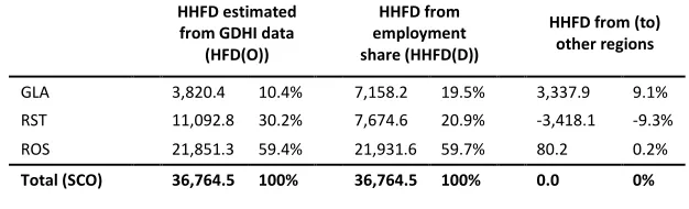
Table 4 Household final demand in Scotland. Origin and destination by

sub-region.

HHFD estimated from GDHI data

(HFD(O))

HHFD from employment share (HHFD(D))

HHFD from (to) other regions

GLA 3,820.4 10.4% 7,158.2 19.5% 3,337.9 9.1%

RST 11,092.8 30.2% 7,674.6 20.9% -3,418.1 -9.3%

ROS 21,851.3 59.4% 21,931.6 59.7% 80.2 0.2%

Total (SCO) 36,764.5 100% 36,764.5 100% 0.0 0%

Table 4 shows this calculation for each region on aggregate. This reveals that

Glasgow is a net-exporter of goods and services that satisfy household final

demand in the rest of the Strathclyde, while the rest of Scotland is largely

21

Strathclyde gets spent in Glasgow, suggesting strong spill-over effects in terms of

Type-II multipliers.

4.4.2 Government demand

The disaggregation of government final demand by sub-region draws on regional

government accounts (Hillis, 1998) and public sector employment by sub-region

to construct weights, which in turn are used to disaggregate the local and central

government final demand columns from the Scottish IO-table11.

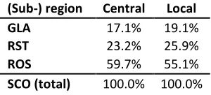
Table 5 Breakdown of central- and local government expenditures by IO

region.

(Sub-) region Central Local

GLA 17.1% 19.1%

RST 23.2% 25.9%

ROS 59.7% 55.1%

SCO (total) 100.0% 100.0%

Table 5 reveals the breakdown of central- and local government expenditures in

each of the 3 IO-regions. Local government expenditures are relatively larger in

GLA and RST, whereas the converse holds for ROS where central government

expenditures are a relatively larger share.

4.4.3 NPISHs, Tourist Demand and Gross Capital Formation

For the disaggregation of NPISHs (Non Profit Institutions Serving Households),

Tourist Demand and the Gross Capital Formation final demand categories a simple

11 _{The latest year the regional government accounts (Hillis, 1998) refer to is 1998. This was a}

22

approach is used. It is assume that demand for each sector is proportional to the

share of Scotland-wide employment in that sector found in Glasgow, such that:













=

i R i N i R i

E

E

F

F

where is a final demand (of an unspecified category) for sector i in region r, '

is the final demand (of the same category) for sector i in Scotland as a whole

(N), 4 is the FTE employment in sector i in region R and 4' is the FTE

employment in sector i in Scotland as a whole (N).

4.4.4 Exports and balancing

As the 3-region table is a disaggregation of the balanced Scottish IO-table it should

by definition balance if constrained to each sector’s row and column total.

Therefore there is no need to apply an adjustment procedure, as the IO-table

conforms to the accounting identity that column sum must equal row sums. As

there is least information available for spatial distribution of RUK and ROW

exports this is chosen as a balancing row. The starting point in this process is

determining the shares of total exports of a sector that go to the RUK and ROW.

For this it is assumed that the RUK/ROW breakdown of exports at the Scottish

level hold at the sub-regional level. Then the total exports of sector i in region r is

determined as that sector’s estimated gross output, less intermediate demand

and less all the final demands estimated so far (i.e. everything but exports). This

estimate for total exports is then attributed to RUK and ROW exports using the

previously determined weights for RUK and ROW exports for sector i. This

concludes the disaggregation process.

23

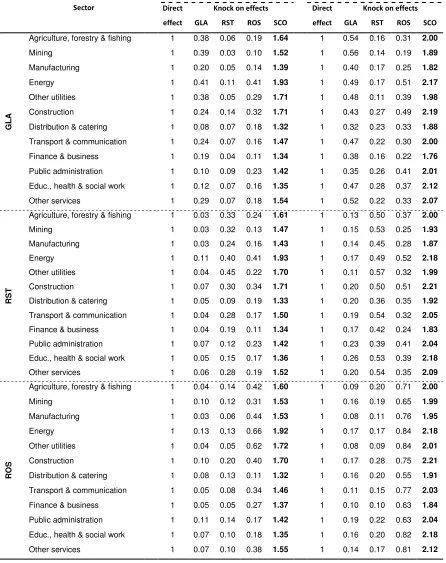
Table 6: Type-I and Type-II interregional multipliers in the interregional

GLA-RST-ROS Input-Output table.

Sector

Type-I multiplier Type-II multiplier

Direct effect

Knock on effects Direct

effect

Knock on effects

GLA RST ROS SCO GLA RST ROS SCO

G

L

A

Agriculture, forestry & fishing 1 0.38 0.06 0.19 1.64 1 0.54 0.16 0.31 2.00

Mining 1 0.39 0.03 0.10 1.52 1 0.56 0.14 0.19 1.89

Manufacturing 1 0.20 0.05 0.14 1.39 1 0.40 0.17 0.25 1.82

Energy 1 0.41 0.11 0.41 1.93 1 0.49 0.17 0.51 2.17

Other utilities 1 0.38 0.05 0.29 1.71 1 0.48 0.11 0.39 1.98

Construction 1 0.24 0.14 0.32 1.71 1 0.43 0.27 0.49 2.19

Distribution & catering 1 0.08 0.07 0.18 1.32 1 0.32 0.23 0.33 1.88

Transport & communication 1 0.24 0.07 0.16 1.47 1 0.47 0.22 0.30 2.00

Finance & business 1 0.19 0.04 0.11 1.34 1 0.38 0.16 0.22 1.76

Public administration 1 0.10 0.09 0.23 1.42 1 0.35 0.26 0.41 2.01

Educ., health & social work 1 0.12 0.07 0.16 1.35 1 0.47 0.28 0.37 2.12

Other services 1 0.29 0.07 0.18 1.54 1 0.52 0.22 0.33 2.07

R

S

T

Agriculture, forestry & fishing 1 0.03 0.33 0.24 1.61 1 0.13 0.50 0.37 2.00

Mining 1 0.03 0.32 0.13 1.47 1 0.15 0.53 0.25 1.93

Manufacturing 1 0.03 0.24 0.16 1.43 1 0.14 0.45 0.28 1.87

Energy 1 0.11 0.40 0.41 1.93 1 0.17 0.49 0.52 2.18

Other utilities 1 0.04 0.45 0.22 1.70 1 0.11 0.57 0.32 1.99

Construction 1 0.07 0.30 0.34 1.71 1 0.20 0.50 0.51 2.21

Distribution & catering 1 0.05 0.09 0.19 1.33 1 0.20 0.36 0.35 1.92

Transport & communication 1 0.04 0.28 0.17 1.50 1 0.19 0.54 0.32 2.05

Finance & business 1 0.04 0.19 0.11 1.34 1 0.17 0.42 0.24 1.83

Public administration 1 0.07 0.12 0.23 1.42 1 0.23 0.39 0.41 2.04

Educ., health & social work 1 0.05 0.15 0.17 1.36 1 0.26 0.53 0.39 2.18

Other services 1 0.06 0.28 0.19 1.52 1 0.20 0.54 0.35 2.09

R

O

S

Agriculture, forestry & fishing 1 0.04 0.14 0.42 1.60 1 0.09 0.20 0.71 2.00

Mining 1 0.10 0.12 0.31 1.53 1 0.16 0.19 0.65 1.99

Manufacturing 1 0.03 0.06 0.44 1.53 1 0.08 0.11 0.76 1.95

Energy 1 0.13 0.13 0.66 1.92 1 0.17 0.17 0.84 2.18

Other utilities 1 0.04 0.05 0.62 1.72 1 0.08 0.09 0.84 2.01

Construction 1 0.10 0.20 0.40 1.70 1 0.17 0.28 0.75 2.21

Distribution & catering 1 0.08 0.13 0.11 1.32 1 0.16 0.20 0.55 1.91

Transport & communication 1 0.05 0.08 0.34 1.46 1 0.11 0.15 0.77 2.03

Finance & business 1 0.05 0.05 0.27 1.37 1 0.10 0.10 0.63 1.84

Public administration 1 0.11 0.14 0.17 1.42 1 0.19 0.22 0.63 2.04

Educ., health & social work 1 0.07 0.10 0.18 1.35 1 0.16 0.20 0.82 2.18

24

The interregional Type-I and Type-II multipliers are shown in a disaggregated

format in Table 6, revealing the direct effect upon the host region and the knock

on effects for each of the 3-regions12 and Scotland as a whole. For example, for

Public Administration in Glasgow the total Scotland-wide Type-II output multiplier

is 2.01. This is composed of the direct effect upon the host region GLA (1) in

addition to knock impacts upon GLA (0.35), RST (0.26) and ROS (0.41). From the

multipliers, it is clear that interregional intermediate trade (indirect effects as

gauged by the Type-I multiplier) drives significant spill-over effects, but that this

varies across sectors and sub-regions. A graphical exposition of this point is

provided in Figure 3.

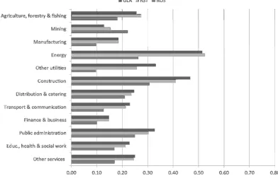
Figure 3 knock-on effects that spill over to other regions by sector and

host-region.

12 _{For ease of exposition the sectors were aggregated from 126 to 12 for each sub-region,}

25

When incorporating induced effects, using the Type-II multipliers, a greater

degree of interregional interdependency is revealed. Figure 4 is identical to Figure

3 and drawn in the same scale to facilitate comparison This reveals the increase in

interregional spill-overs of knock-on effects, once induced effects are accounted

for in addition to indirect effects. Again, the individual sub-regions differ in the

extent to which host-region demand stimuli spill over to the other regions. In this

regards GLA and RST are clearly more open than the larger ROS.

Figure 4 Type-II knock-on effects that spill over to other regions by sector

and host-region.

5

Alternative specifications and sensitivity of

multipliers

Sensitivity analysis is conduced around two dimensions: the approach used to

26

impacts; and the treatment of wages and household consumption, which

influence the nature of induced impacts.

5.1

Intermediate transactions

The IO-table is estimated using alternative LQs. The FLQ formula is used under a

range of δ parameters and compared to a version of the IO-table estimated using

SLQs. Three parameter values are chosen. To simplify the presentation of results

the industrial sectors are aggregated into 1 sector for each region. These are

presented in Table 7. Which shows these aggregate multipliers broken down into

their constituent components: direct effect, local knock-on effect and

interregional knock-on effect.

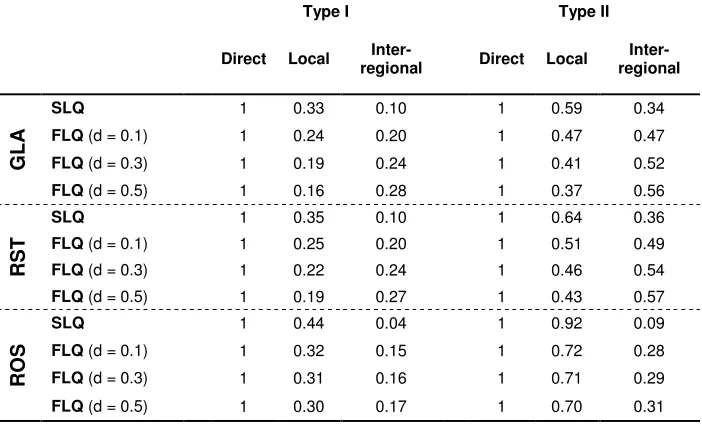
Table 7 Spatial decomposition of aggregate multipliers by sub-region

Type I Type II

Direct Local Inter-

regional Direct Local

Inter- regional

G

L

A

SLQ 1 0.33 0.10 1 0.59 0.34

FLQ (d = 0.1) 1 0.24 0.20 1 0.47 0.47

FLQ (d = 0.3) 1 0.19 0.24 1 0.41 0.52

FLQ (d = 0.5) 1 0.16 0.28 1 0.37 0.56

R

S

T

SLQ 1 0.35 0.10 1 0.64 0.36

FLQ (d = 0.1) 1 0.25 0.20 1 0.51 0.49

FLQ (d = 0.3) 1 0.22 0.24 1 0.46 0.54

FLQ (d = 0.5) 1 0.19 0.27 1 0.43 0.57

R

O

S

SLQ 1 0.44 0.04 1 0.92 0.09

FLQ (d = 0.1) 1 0.32 0.15 1 0.72 0.28

FLQ (d = 0.3) 1 0.31 0.16 1 0.71 0.29

FLQ (d = 0.5) 1 0.30 0.17 1 0.70 0.31

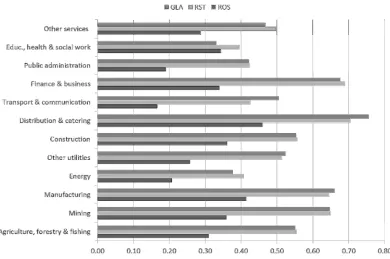
A graphical summary of these results is presented Figure 5 below. The horizontal

bars identify the interregional component of the multiplier of the aggregate

sector in each region, based on estimates using alternative LQ specifications.

Looking at the Type-I multipliers, the difference between the estimated results

27

assumption of FLQ (δ=0.3), for every £1 of final demand stimulus locally there

would be an interregional spill-over effect of 24p, whereas under the SLQ this

would only be 10p. Varying the δ parameter does vary the outcome, but this

sensitivity is much less distinct than the initial choice between SLQ and FLQ.

Furthermore, there is a clear qualitative distinction between results obtained in

the smaller more open sub-regions of GLA and RST, vis-á-vis the larger and more

self-contained ROS. In the latter case spill-over effects are much less distinct, 16p

in the pound for the baseline assumptions, but only 4p based on SLQs.

Figure 5 Knock-on impacts that spill over across sub-regional boundaries

under alternative LQ-formulas.

As expected, the Type-II multipliers reveal larger spill-over effects. For example,

based on the base case assumption a £1 of final demand stimulus in Glasgow will

result in 52p of knock-on impacts in the other two sub-regions. Again, these

28

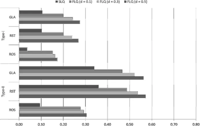
5.2

Household incomes and expenditures

As is detailed in section 4.3 and 4.4.1 this paper adopts a simple method to allow

for interregional flows of wages and consumption. For comparison the table was

re-estimated using a typical LQ-type approach, where all employment is assumed

to be local and all household consumption is assumed to occur locally. The results

indicate that allowing for these drivers of spill-over effects, is important when

looking at smaller geographical units. Figure 6 reveals that under

‘origin-destination’ assumptions for wages and consumption each £1 of final demand

stimulus in GLA and RST leads to spill-over effects of 52 and 54p respectively.

Whereas, under the ‘standard’ assumptions, these spill-over impacts would be

reduced to 42p and 39p respectively. However, for the larger ROS the

specification of the income and expenditures of the household sector is not

important.

Figure 6 Comparison of the interregional knock-on impacts of aggregate

sectors, based on a ‘standard’ treatment of household incomes/expenditures

29

Figure 7 Presents the same comparison disaggregated to 12 sectors in each

sub-region. This suggests that an accurate treatment of the household is most

important for those sectors that are most labour intensive.

Figure 7 Comparison between the interregional component of the multiplier

based on a ‘standard’ treatment of household incomes-expenditures and an

origin-destination treatment acknowledging interregional commuter and

30

6

Conclusions

This paper explores the sensitivity of multipliers to assumptions adopted when

constructing local Input-Output tables using non-survey methods. The official

Scottish IO-table is spatially disaggregated to identify interdependencies between

the largest city, Glasgow, its wider city-region in the rest of the Strathclyde region

and the wider regional economy in the rest of Scotland. Once the base case has

been established sensitivity analysis is conducted around two dimensions: the

specification of intermediate inputs and the flow of wages and household

consumption. The analysis supports existing finding in the literature that accurate

estimation of intermediate trade is important if multipliers are not to be

overstated. However, it further argues that researchers need also to think about

accurate estimation of wage and consumption flows if Type-II multipliers are not

to be overstated (and spill over effects underestimated when working a

multi-region context). This is particularly important when working at smaller scales

where commuting and shopping trips occur beyond the study area. Glasgow

exemplifies this situation with 40% of jobs taken by in-commuters and conversely,

about a quarter of all household consumption in its wider city-region is spent

within the city. However, these concerns are not urgent when looking at larger

geographical areas, such as is exemplified by results for the rest of Scotland.

The results clearly indicate that researchers must adopt a wider stance than solely

focussing on trade when constructing local level IO tables. Given that these results

are based on simulation it would be highly desirable to verify them through

empirical testing. However, this is not possible for the case of Glasgow, as a fully

surveyed benchmark table is lacking. There are several local economy tables

31

and therefore not suitable to test for the impact of commuting and shopping trips

when using non-survey methods to estimate local level IO-tables.

The interregional IO table features a simple mechanism that utilises secondary

data to capture wage and consumption flows over regional boundaries. This is a

significant improvement over conventional approaches but still suffers

weaknesses, which would require more detailed data to address. In particular it

would be useful to obtain sector specific commuting intensities and more detailed

picture of interregional flows of household consumption. The first of these could

be achieved with further disaggregation of census results but the latter does not

have an obvious solution short of extensive primary data collection. A possible

solution might be making use of data on card payments, which are stored in great

32

References

Batten, D. (1982). The Interregional Linkages between National and Regional

Input-Output Models. International Regional Science Review. Vol. 7, No. 1, pp.

53-67.

Bonfiglio A. (2009) On the Parameterization of Techniques for Representing

Regional Economic Structures. Economic Systems Research. Vol. 21, pp. 115−127.

Brand, S. (1997). On the Appropriate Use of Location Quotients in Generating

Regional Input-Output Tables: A Comment. Regional Studies, Vol. 31.8, pp.

791-794.

Flegg, A.T, & Tohmo, T. (2011). Regional Input–Output Tables and the FLQ

Formula: A Case Study of Finland. Regional Studies. DOI:

http://dx.doi.org/10.1080/00343404.2011.592138

Flegg. A.T., Webber, C.D. & Elliott, M.V. (1995). On the appropriate use of location

quotients in generating regional input-output tables. Regional Studies, Vol. 29,

No. 6, pp. 547-561.

Flegg, A.T. & Webber, C.D. (1996). Using Location Quotients to Estimate Regional

Input-Output Coefficients and Multipliers. Local Economy Quarterly. Vol. 4, pp.

58-86.

Flegg, A.T. & Webber, C.D. (1997). On the appropriate use of location quotients in

generating regional input-output tables: Reply. Regional Studies, Vol. 31, No. 8,

33

Flegg, A.T. & Webber, C.D. (2000). Regional size, regional specialisation and the

FLQ formula. Regional Studies. Vol. 34, No. 6, pp. 563-569.

Flegg, A.T & Tohmo, T. (2010). Regional Input-Output Tables and the FLQ Formula:

A Case Study of Finland. University of the West of England, Department of

Economics, Discussion Paper. Retrieved from the World Wide Web:

http://carecon.org.uk/DPs/1005.pdf

Fleming, A.D. (2006). Scotland’s Census 2001 Statistics on Travel to Work or Study.

General Register Office for Scotland. Occasional Paper No. 12.

Harrigan, F., McGilvray, J.W. & McNicoll, I.H. (1980a). Simulating the Structure of a

Regional Economy. Environment and Planning A. Vol.12, pp. 927-36.

Harrigan, F., McGilvray, J., & McNicoll, I. (1980b). A comparison of regional and

national technical structures. The Economic Journal, 90(360), 795-810.

Harris, R.I.D. & Liu, A. (1998). Input-Output Modelling of the Urban and Regional

Economy: The Importance of External Trade. Regional Studies, Vol. 32, No. 9, pp.

851-862.

Hillis, I. (1998). Sub Regional Government Accounts (experimental). Office for

National Statistics (ONS). Retrieved from the World Wide Web:

http://www.statistics.gov.uk/statbase/Product.asp?vlnk=9580&More=Y

Lahr, M.L. (1993). A Review of the Literature Supporting the Hybrid Approach to

Constructing Regional Input-Output Models. Economic Systems Research. Vol. 5,

34

Lahr, M. & de Mesnard, L. (2004). Biproportional Teqhniques in Input-Output

Analysis: Table Updating and Structural Analysis. Economic Systems Research. Vol.

16, No. 2, pp. 115-134.

Norcliffe, G.B. (1983. Using location quotients to estimate the economic base and

trade flows. Regional Studies. Vol. 17, No. 3. pp. 161-168.

McCann, P. & Dewhurst, J. (1998). Regional Size, Industrial Location and

Input-Output Expenditure Coefficients. Regional Studies, Vol. 32.5, pp. 435-444.

Miller, R.E. & Blair, P.D. (1985). Input-Output Analysis: Foundations and

Extensions, 1st. edition. Prentice Hall.

Miller, R.E. & Blair, P.D. (2009). Input-Output Analysis: Foundations and

Extensions, 2nd edition. Cambridge: Cambridge University Press.

Oosterhaven, J. & Stelder, D. (2007). Regional and Interregional IO Analysis.

Monograph: University of Groningen, Faculty of Economics and Business.

Richardson, H. W. 1985. Input-Output and economic base multipliers: Looking

backward and forward. Journal of Regional Science Vol. 25, No. 4, pp. 607-61.

Roberts, D.J. (2005). The role of households in sustaining rural economies: A

structural path analysis. European Review of Agricultural Economics, vol 32, no. 3,

pp. 393-420.

Robison, M.H. (1997). Community input-output models for rural area analysis with

35

Robison, M.H. & Miller, J.R. (1988). Cross-Hauling and Nonsurvey Input-Output

Models: Some Lessons from Small-Area Timber Economies. Environment and

Planning A, Vol. 20, pp. 1523-1530.

Robison, M.H. & Miller, J.R. (1991). Central Place Theory and Intercommunity

Input-Output Analysis. Papers in Regional Science. Vol. , No. 4, pp. 399-417.

Round, J.I. (1978). An Interregional Input-Output Approach to the Evaluation of

Nonsurvey Methods. Journal of Regional Science. Vol. 18, No. 2., pp. 179-194.

Schaffer, W.A. & Chu, K. (1969). Nonsurvey Techniques for Constructing Regional

Interindustry Models. Papers in Regional Science. Vol. 23, No. 1, pp. 83-104.

Smith, P. & Morrison, W.I. (1974). Simulating the Urban Economy: Input-Output

Techniques. Pion, London.

Snickars, F. (1979). Construction of Interregional Input Iutput Tables by Efficient

Information Adding. In Bartels, C.P.A. & Ketellapper, R.H. (eds). Exploratory and

Explanatory Statistical Analysis of Spatial Data. Berlin: Springer.

Snickars, F. & Weibull, J.W. (1977). A Minimum Information Principle: Theory and

Practice. Regional Science and Urban Economics. Vol. 7, pp. 137-168.

Stoeckl, N. (2010). International Regional Science Review. Comparing Multipliers

from Survey and Non-Survey Based IO Models: An Empirical Investigation from

Northern Australia. International Regional Science Review. Published online

36

Tohmo, T. (2004). New Developments in the Use of Location Quotients to

Estimate Regional Input-Output Coefficients and Multipliers. Regional Studies,

Vol. 381, No. 1, pp. 45-54.

Willis, K.G. (1987). Spatially disaggregated input-output tables: an evaluation and

comparison of survey and nonsurvey results. Environment and Planning A.

Volume 19, pp. 107-116.