3D-RISM
Maksim Misin,1Maxim V. Fedorov,1,a)and David S. Palmer2,b) 1)
Department of Physics, SUPA, University of Strathclyde, 107 Rottenrow, Glasgow, G4 0NG, UK
2)Department of Pure and Applied Chemistry, University of Strathclyde, 16 Richmond Street, Glasgow, G1 1XQ,
UK
(Dated: 23 February 2015)
We present a new model for computing hydration free energies by 3D-RISM that uses an appropriate ini-tial state of the system (as suggested by Sergiievskyi et al.). The new adjustment to 3D-RISM theory significantly improves hydration free energy predictions for various classes of organic molecules at both am-bient and non-amam-bient temperatures. An extensive benchmarking against experimental data shows that the accuracy of the model is comparable to (much more computationally expensive) molecular dynamics simu-lations. The calculations can be readily performed with a standard 3D-RISM algorithm. In our work we used an open source package AmberTools; a script to automate the whole procedure is available on the web (https://github.com/MTS-Strathclyde/ISc).
I. INTRODUCTION
Hydration free energy, ∆Ghyd, is one of the most important properties in solution chemistry. It pro-vides information about the partitioning of a solute be-tween gas and solution phases and is used in calculating solubility1–3, acid-base dissociation constant4,
octanol-water partition coefficient5, and protein-ligand binding
free energy6, amongst other properties. The hydration
free energies of non-ionic organic solutes can be computed using molecular dynamics (MD) simulations with an ac-curacy approaching that of experiments.7. However, for
many purposes (in particular for high-throughput screen-ing over large digital libraries of compounds) the MD approach is not ideal as it requires large computational resources7–9. Additionally, the large number of existing MD methods and the variety of input parameters both for the model itself (molecular geometry, force-field, number of molecules in the simulation box, etc) and for the sim-ulation protocol (time step, MD integrator, thermostat, barostat, equilibration time etc) together with the need to use a parallel computer architecture makes it difficult for non-specialists to perform these calculations.
The 3D Reference Interaction Site Model (3D-RISM) is a molecular theory closely related to classical DFT10–13.
It describes the local solvent density around a solute using 3D spatial solute-solvent distribution functions, which are obtained via iterative solution of a system of integral equations. Using 3D-RISM one can compute a range of thermodynamic properties as well as struc-tural information about the solvent in a relatively short time (on the order of a few minutes)14–17. In princi-ple it can be applied to arbitrary solvent compositions and temperatures18–20,72–74. However, despite recent
ad-vances, such as the introduction of semi-empirical free
a)Electronic mail: maxim.fedorov@strath.ac.uk b)Electronic mail: david.palmer@strath.ac.uk
energy functionals,15,21–24 the accuracy of theory-based 3D-RISM methods (i.e. those without empirical correc-tions) has remained low25.
In this paper we build upon recent theoretical work by Sergiievskyiet al.25and propose a new correction for the 3D-RISM hypernetted-chain (3D-RISM/HNC) the-ory. To assess the strengths and limitations of the new model, we compare its predictions to experimental hydra-tion free energy data for small organic molecules at both ambient and non-ambient temperatures. We show that the new term not only improves predictions at 298 K, but also makes the error practically temperature-independent for the range of temperatures between 278 K and 378 K that were studied here.
II. THEORY
An important part of 3D-RISM theory is the so called closure expression. It provides a connection between in-tramolecular potentialu(r) and distribution functions:
h(r) + 1 = exp(−βu(r) +h(r)−c(r) +B(r)) (1)
hereh(r) is the total correlation function,c(r) is the di-rect correlation function, andB(r) is a bridge function, defined using diagrammatic expansion14,26–29. In prac-tice however, one often substitutesB(r) with various ap-proximations.
A common choice is to set B(r) = 0 in the so called hypernetted-chain approximation (HNC). How-ever, this approach suffers from poor computational convergence30,31. This problem can be reduced by the use of a partial series expansion of order n (PSE-n) of the HNC closure30:
h(r) =
n P
i=0
Ξi(r)/i!−1 if Ξ(r)>0
exp (Ξ(r))−1 if Ξ(r)≤0
where Ξ(r) =−βu(r) +h(r)−c(r). Settingn= 1 results in the partial linearized closure proposed by Kovalenko and Hirata (KH)26,27— a remarkably numerically stable
closure. n→ ∞ gives the HNC closure and its conver-gence issues. PSE-3 achieves a good balance between the two: it has been found to have good convergence and it gives results that approximate HNC predictions well30. Due to these properties PSE-3 and other PSE-n closures have been extensively applied for a variety of charged and biomolecular systems32–35.
For both HNC and its n-order expansions, the excess chemical potential of the solute at infinite dilution, µex
can be derived from the RISM solute-solvent correlation functions14,30,36,37. For the HNC closure, the functional
is14:
µexHN C=kT N sites
X
α=1
ρα Z
V
1 2h
2
α(r)−cα(r)−
1
2cα(r)hα(r)
dr
(3)
where ρα is the number density of solvent sites α. For PSE-n closure30:
µexP SE−n =µexHN C−kT
N sites X
α=1
ρα
Z
V h
Θ (hα(r)) (Ξα(r))n+1/(n+ 1)! i
dr
(4)
[image:2.612.62.286.520.622.2]where Θ is a Heaviside step function. Unfortunately, ∆Gs computed by 3D-RISM with the use of these ex-pressions as ∆Gs = µexRISM, have a large positive bias and standard deviation when compared to available ex-perimental data25.
FIG. 1. Illustration of different reference states. The style of the figure is inspired by Figure 1 from Ref. 25. ∆V here is the partial molar volume of the solute and ∆N = ∆V ρ.
In a recent paper, Sergiievskyiet al. have shown that ∆Gs predictions by molecular theories like Molecular Density Functional Theory (MDFT) and 3D-RISM can be improved by introducing a correction to transform the results from the grand canonical to the isobaric-isotherm ensemble25. We follow the idea from that paper in our derivation of the proper correction for ∆Gscalculated by 3D-RISM.
The main idea behind the correction is that the original 3D-RISM is defined for the grand canonical ensemble28,
meaning that it computes the solute excess chemical po-tential with regards to state 1 (figure 1; state 1 is the initial state with N+ ∆N water molecules and volume
V). However, experiments and MD simulations compute the free energy difference between states 2 and 0 (figure 1; state 2 is the final state withN water molecules and volume V, state 0 has N water molecules and V −∆V
volume).
A derivation of the initial state correction for the MDFT case is given in Ref. 25. Following the main re-sult of that paper, the ∆Gsbetween states 2 and 0, when computed by 3D-RISM, takes the following form:
∆Gs,ISc=µexRISM −ρkT∆V +ρ 2kT
2 cˆ(k= 0)∆V (5)
where ρ is the density of the bulk solvent, ∆V stands for the partial molar volume, and ˆc(k = 0) is the value of the Fourier transformed direct correlation function of pure water at k=0 (it can be obtained from 1D-RISM calculation and expressed using the pure solvent isother-mal compressibility: ρˆc(k= 0) = 1−1/(ρkT χT))25. We will refer to this expression as the Initial State correction (ISc).
After deriving the equation 5, Sergiievskyiet al.argue that the ∆Gshas an extra contribution due to the change in the chemical potential of solvent (as a result of the increase in volume) equal toρkT∆V. They propose the following formula for computing the solvation free energy:
∆Gs,ISc∗=µexRISM+ρ2 kT
2 cˆ(k= 0)∆V (6)
For simplicity we will refer to this expression as ISc∗. This is the formula which was used in Ref. 25 to estimate the accuracy of the corrected 3D-RISM/HNC.
Equation 6 was originally developed for MDFT, not for 3D-RISM. However, the 3D-RISM is actually defined for the case of grand canonical ensemble14,28 meaning that the solvent potential is imposed by the outside reservoir; therefore, there should be no change in chemical poten-tial of the solvent due to an increase in volume. Con-sequently, we argue that for 3D-RISM the ISc formula (equation 5) has to be used to correct the solvation free energies.
To support our statement we will present below results of an extensive benchmarking of both the ISc∗(equation 6) and the ISc (equation 5) formulae for calculating sol-vation free energy in bulk water (hydration free energy) of various organic molecules at a range of different tem-peratures.
III. METHODS
To evaluate the performance of the ISc and
the ISc∗ models at 298 K, we have used a
for small organic molecules compiled by Mobley
et al.39 The original dataset contained 504 molecules,
but we found that two molecules were
dupli-cated (”3 methyl but 1 ene”/”3 methylbut 1 ene” and ”2 methyl but 2 ene”/”2 methylbut 2 ene”). All com-pounds in the dataset are non-ionic, with an average molecular mass of 113 g/mol and an average logP of 1.7 (logP was estimated using the RdKit40
implemen-tation of the Wildman-Crippen algorithm41). In
addi-tion to the molecular structures and experimental data, the dataset also includes free energies obtained using the Bennett Acceptance Ratio method42 from MD simula-tions performed with the Generalized Amber Forcefield (GAFF)43, AM1-BCC44 charges, and TIP3P water45.
The dataset with hydration free energies at varied tem-peratures was kindly granted to us by C.J. Cramer.46,47
The dataset contains measurements of hydration free en-ergy for a variety of small, non-ionic organic molecules in a broad temperature range and was used for parametriza-tion of the SM6T and SM8T solvaparametriza-tion models46,47. For simplicity, we will refer to this dataset by the name of the first author of the publications: the Chamber-lin dataset. The experimental hydration free energy data in both datasets used here are given as ∆Gexphyd =
−RTlncaq/cgas, with concentrations in mol/L, which corresponds to the choice of standard states suggested by Ben-Naim48,49. The raw version of the Chamberlin
dataset contained measurements collected from various sources. To identify and eliminate possible systematic and random errors in this data, we have adopted a strat-egy similar to that used in the original publications (Ref. 46 and 47). We have carefully described our steps in the supporting information. The final version of the dataset contains 272 molecules with 3053 hydration free energy data points measured at temperatures between 273K and 373K; many values were averaged over multiple experi-mental measurements. The average molecular mass of the molecules in the dataset is 107 g/mol, average logP is 1.6. Both Chamberlin and Mobley datasets, including the structures of the molecules that we used, are provided in the supporting information50.
The initial geometry guess for each molecule was cre-ated using the Openbabel software package51,52. After that, for each molecule we performed a conformational search with the OPLS 2005 force field53using the mixed
torsional/low-mode sampling method as implemented in Macromodel54. For subsequent calculations, we used
only the lowest energy conformation for each molecule. The data analysis and plotting was accomplished us-ing the Scientific Python software stack55–58. Molecular
structures were visualized using RDKit and Marvin40,59.
For all calculations we used a modified SPC/E water model (cSPC/e, see Ref. 60 for details) with oxygen par-tial charge of −0.8476, σO = 3.16572 ˚A, σH = 1.16572 ˚
A, O = 0.1553 kcal/mol, H = 0.01553 kcal/mol. For all the solutes Lennard-Jones parameters were taken from the general amber force field (GAFF)43and partial charges were generated using the AM1-BCC scheme44.
The water susceptibility functions were generated us-ing the DRISM program14,27,60 included in the
Amber-Tools 13 package61. The set of input parameters
sisted of temperature, water density and dielectric con-stants. The latter two parameters were obtained us-ing interpolation functions provided in the Water Soci-ety manual62 (the relative uncertainty of the density is around 0.0001% and for the dielectric constant is 0.01 % ). The DRISM equations were solved with tolerance set to 1×10⁻¹²and grid spacing to 0.025 ˚A.
All 3D-RISM calculations were performed using the rism3d.snglpnt program from AmberTools 13 package. The grid spacing was set to 0.3 ˚A buffer to 30 ˚A and tolerance to 1×10⁻¹⁰. These parameters were found
to converge even for rather big systems23. All
calcula-tions were performed twice, with both HNC and PSE-3 bridge closures. The outputs obtained with different clo-sures were not mixed, meaning that DRISM, 3D-RISM and hydration free energy evaluations were done using formulas specific to a particular closure. Integral equa-tions were solved numerically using a modified DIIS algo-rithm to speed up convergence63. To automate the
cal-culation procedure we created a Python script, which we have made freely available at https://github.com/MTS-Strathclyde/ISc.
IV. RESULTS AND DISCUSSION
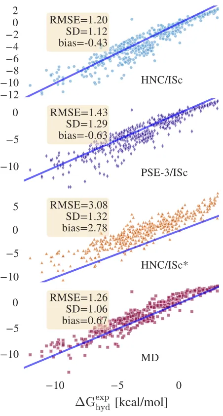
Figure 2 shows the accuracies of four different models on the 298 K dataset composed by Mobley et al. Re-markably, HNC/ISc achieves an accuracy equivalent to the MD simulations which used the same force field and partial charges (the MD data were taken from Ref. 39). While the HNC/ISc∗’s standard error is not much bigger, it has a large positive bias, providing a justification for our approach to the correction ofµex
RISM.
Due to the above mentioned problems, calculations with HNC closure did not converge for 25 molecules (details are provided in the supporting information). On the other hand, all the PSE-3/ISc calculations con-verged with an accuracy only slightly worse than that for HNC/ISc. This suggest that PSE-3/ISc may be a practical alternative to HNC/ISc calculations for many systems of chemical interest.
The results predicted by both HNC/ISc and PSE-3/ISc are similar to MD: the correlation coefficient is
FIG. 2. Hydration free energies predicted by HNC/ISc, PSE-3/ISc, HNC/ISc∗, and MD against experimental data from the Mobley dataset at 298 K. The blue line is a graph of the function y=x.
−12
−10
−8
−6
−4
−2
0
2
¢
G
HN
C
=
IS
c
RMSE=1.20
SD=1.12
bias=-0.43
HNC/ISc
−10
−5
0
¢
G
PS
E
¡
3
=
IS
c
RMSE=1.43
SD=1.29
bias=-0.63
PSE-3/ISc
−10
−5
0
5
¢
G
HN
C
=
IS
c
¤
RMSE=3.08
SD=1.32
bias=2.78
HNC/ISc*
−10
−5
0
¢G
exphyd[kcal/mol]
−10
−5
0
¢
G
MD
RMSE=1.26
SD=1.06
bias=0.67
MD
Careful examination of Figure 2 shows that ISc models perform somewhat worse than MD for hydrophilic com-pounds. This is most likely caused by shortcomings of the bridge closure. Essentially, the correction presented here only addresses errors due to excluded volume effects, the problems due to the exclusion of higher order bridge terms are still present. This issue might be addressed using more advanced bridges, of which the method pro-posed by Duh and Henderson is one such example71. This
is the subject for future work.
It should be noted that the functional form of the model presented here is similar to another 3D-RISM hy-dration free energy correction published by Palmeret al.
in Ref. 21: ∆Gs,U C = µexRISM,KH +aρ∆V +b. Here
a = −3.312 kcal/mol and b = 1.152 kcal/mol are fit-ted coefficients for water solvent. Rearranging the ISc model into similar form gives us a = −3.673 kcal/mol andb= 0 kcal/mol for aqueous solvent at standard con-ditions. The correction by Palmer et al. gives similar accuracy forambient conditions. However, ISc similarly to 3D-RISM can be applied to a system at arbitrary tem-peratures and pressures. Therefore, to provide additional insights into the validity of the ISc and ISc∗ models we performed benchmarks for each model at different tem-peratures.
[image:4.612.322.546.349.545.2]To the best of our knowledge, there have been no re-ports investigating the performance of the 3D-RISM or a similar model at a wide range of temperatures for a large dataset of compounds from different chemical classes. Therefore, the benchmark provides a landmark for ex-isting molecular theories of solvation.
FIG. 3. RMSE of hydration free energies of HNC/ISc (blue columns), PSE-3/ISc (violet columns) and HNC/ISc∗(orange columns) depending on temperature. The bold lines on top of the bars are standard uncertainties (the equation is provided in the Supporting Information). The experimental data are taken from Chamberlin dataset.46,47
278 288 298 308 318 328 338 348 358 368
Temperature [K]
0
1
2
3
4
RMSE [kcal/mol]
HNC=ISc PSE¡3=ISc
HNC=ISc¤
At most temperatures, ISc models are almost twice as accurate as ISc∗. Additionally, ISc∗ becomes less reli-able towards higher temperatures, while the ISc errors remains essentially constant for all temperatures. This is another indication that supports the validity of the ISc over the ISc∗ model.
The error of the ISc models at 298 K is slightly higher (about 1.5 kcal/mol) for the Chamberlin dataset than for the Mobley dataset (3). This difference seems to orig-inate from differences in the molecules as well as the sources of experimental data. It is hard to determine which data are more accurate as experimental uncertain-ties were not published with either dataset. As in the case of ambient temperature dataset, PSE-3/ISc results are only slightly worse than HNC/ISc ones, but have an ad-vantage due to greater numerical stability: calculations with HNC bridge didn’t converge in 121 cases (more de-tails are provided in the supporting information).
To summarize, this letter describes a new, 3D-RISM theory based on the initial state correction (ISc). In con-trast to the models that use semi-empirical corrections like the ones described in Refs 15,21,22 this model does not require additional training and/or extensive parame-terisation. At the same time, the ISc models predict the hydration free energy for a wide set of organic molecules with a good accuracy both at ambient and non-ambient temperatures. In terms of accuracy the model performs best when combined with HNC; however, much better numerical stability with only a slight decrease in accu-racy can be achieved with the PSE-3 closure.
ACKNOWLEDGMENTS
We are grateful to Fumio Hirata for valuable dis-cussions about the theoretical foundations of the 3D-RISM and to Volodymyr Sergiievskyi and Daniel Borgis for helpful discussions about the corrected MDFT theory. Results were obtained using the EP-SRC funded ARCHIE-WeSt High Performance Com-puter (www.archie-west.ac.uk). EPSRC grant no. EP/K000586/1. DSP is grateful for funding from the European Commission through a Marie Curie Intra-European Fellowship within the 7th Intra-European Commu-nity Framework Programme (FP7-PEOPLE-2010-IEF) and to the University of Strathclyde for support through its Strategic Appointment and Investment Scheme.
1J. D. Thompson, C. J. Cramer, and D. G. Truhlar, “Predicting
aqueous solubilities from aqueous free energies of solvation and experimental or calculated vapor pressures of pure substances,” J. Chem. Phys.119, 1661–1670 (2003).
2D. S. Palmer, A. Llin`as, I. Morao, G. M. Day, J. M. Goodman,
R. C. Glen, and J. B. O. Mitchell, “Predicting intrinsic aqueous solubility by a thermodynamic cycle,” Mol. Pharmaceutics 5, 266–279 (2008).
3D. S. Palmer, J. L. McDonagh, J. B. O. Mitchell, T. van Mourik,
and M. V. Fedorov, “First-principles calculation of the intrinsic aqueous solubility of crystalline druglike molecules,” J. Chem. Theory Comput.8, 3322–3337 (2012).
4R. Casasnovas, J. Ortega-Castro, J. Frau, J. Donoso, and
F. Mu˜noz, “Theoretical pKa calculations with continuum model solvents, alternative protocols to thermodynamic cycles,” Int. J. Quantum Chem.114, 1350–1363 (2014).
5N. M. Garrido, A. J. Queimada, M. Jorge, E. A. Macedo, and
I. G. Economou, “1-Octanol/Water partition coefficients of n-alkanes from molecular simulations of absolute solvation free en-ergies,” J. Chem. Theory Comput.5, 2436–2446 (2009).
6D. S. Palmer, J. Sørensen, B. Schiøtt, and M. V. Fedorov,
“Sol-vent binding analysis and computational alanine scanning of the bovine Chymosin–Bovineκ-casein complex using molecular inte-gral equation theory,” J. Chem. Theory Comput.9, 5706–5717 (2013).
7N. Hansen and W. F. van Gunsteren, “Practical aspects of
free-energy calculations: A review,” J. Chem. Theory Comput.10, 2632–2647 (2014).
8C. Chipot and A. Pohorille, Free Energy Calculations: Theory
and Applications in Chemistry and Biology(Springer Science & Business Media, Paris, France, 2007).
9M. R. Shirts and D. L. Mobley, “An introduction to best
prac-tices in free energy calculations,” in Biomolecular Simulations, Methods in Molecular Biology No. 924, edited by L. Monticelli and E. Salonen (Humana Press, Totowa, NJ, 2013) pp. 271–311.
10D. Beglov and B. Roux, “Solvation of complex molecules in a
polar liquid: An integral equation theory,” J. Chem. Phys.104, 8678–8689 (1996).
11D. Beglov and B. Roux, “Numerical-solution of the
hypernetted-chain equation for a solute of arbitrary geometry in 3 dimen-sions,” J. Chem. Phys.103, 360–364 (1995).
12A. Kovalenko and F. Hirata, “Potential of mean force between
two molecular ions in a polar molecular solvent: A study by the three-dimensional reference interaction site model,” J. Phys. Chem. B103, 7942–7957 (1999).
13A. Kovalenko and F. Hirata, “Self-consistent description of a
metal-water interface by the kohn-sham density functional the-ory and the three-dimensional reference interaction site model,” J. Chem. Phys.110, 10095–10112 (1999).
14F. Hirata, ed.,Molecular Theory of Solvation(Kluwer Academic
Publishers, Amsterdam, Netherlands, 2003).
15J.-F. Truchon, B. M. Pettitt, and P. Labute, “A cavity
cor-rected 3D-RISM functional for accurate solvation free energies,” J. Chem. Theory Comput.10, 934–941 (2014).
16Y. Maruyama, N. Yoshida, H. Tadano, D. Takahashi, M. Sato,
and F. Hirata, “Massively parallel implementation of 3D-RISM calculation with volumetric 3D-FFT,” J. Comput. Chem. 35, 1347–1355 (2014).
17V. P. Sergiievskyi and M. V. Fedorov, “3DRISM multigrid
al-gorithm for fast solvation free energy calculations,” J. Chem. Theory Comput.8, 2062–2070 (2012).
18Y. Harano, H. Sato, and F. Hirata, “Solvent effects on a
diels-alder reaction in supercritical water: RISM-SCF study,” J. Am. Chem. Soc.122, 2289–2293 (2000).
19T. Imai, M. Kinoshita, and F. Hirata, “Salt effect on stability
and solvation structure of peptide: An integral equation study,” Bull. Chem. Soc. Jpn.73, 1113–1122 (2000).
20M. Kinoshita, Y. Okamoto, and F. Hirata, “Peptide
conforma-tions in alcohol and water: Analyses by the reference interaction site model theory,” J. Am. Chem. Soc.122, 2773–2779 (2000).
21D. S. Palmer, A. I. Frolov, E. L. Ratkova, and M. V. Fedorov,
“Towards a universal method for calculating hydration free en-ergies: a 3D reference interaction site model with partial mo-lar volume correction,” J. Phys.: Condens. Matter22, 492101 (2010).
22D. S. Palmer, A. I. Frolov, E. L. Ratkova, and M. V. Fedorov,
“Toward a universal model to calculate the solvation thermody-namics of druglike molecules: The importance of new experimen-tal databases,” Mol. Pharmaceutics8, 1423–1429 (2011).
23A. I. Frolov, E. L. Ratkova, D. S. Palmer, and M. V. Fedorov,
(2011).
24E. L. Ratkova and M. V. Fedorov, “Combination of RISM and
cheminformatics for efficient predictions of hydration free energy of polyfragment molecules: Application to a set of organic pol-lutants,” J. Chem. Theory Comput.7, 1450–1457 (2011).
25V. P. Sergiievskyi, G. Jeanmairet, M. Levesque, and D. Borgis,
“Fast computation of solvation free energies with molecular den-sity functional theory: Thermodynamic-ensemble partial molar volume corrections,” J. Phys. Chem. Lett.5, 1935–1942 (2014).
26A. Kovalenko and F. Hirata, “Potentials of mean force of simple
ions in ambient aqueous solution. II. solvation structure from the three-dimensional reference interaction site model approach, and comparison with simulations,” J. Chem. Phys.112, 10403–10417 (2000).
27A. Kovalenko and F. Hirata, “Potentials of mean force of simple
ions in ambient aqueous solution. i. three-dimensional reference interaction site model approach,” J. Chem. Phys.112, 10391– 10402 (2000).
28J.-P. Hansen and I. R. McDonald,Theory of Simple Liquids, 4th
ed. (Academic Press, San Diego, CA, 2013).
29G. N. Chuev and M. V. Fedorov, “Wavelet algorithm for solving
integral equations of molecular liquids. a test for the reference interaction site model,” J. Comput. Chem.25, 1369–1377 (2004).
30S. M. Kast and T. Kloss, “Closed-form expressions of the
chem-ical potential for integral equation closures with certain bridge functions,” J. Chem. Phys.129, 236101 (2008).
31M. Kinoshita and M. Harada, “Numerical solution of the RHNC
theory for water-like fluids near a macroparticle and a planar wall,” Mol. Phys.81, 1473–1488 (1994).
32T. Luchko, I. S. Joung, and D. A. Case, “Integral equation theory
of biomolecules and electrolytes,” inInnovations in Biomolecular Modeling and Simulations, Vol. 1, edited by T. Schlick (Royal Society of Chemistry, London, UK, 2012) pp. 51–86.
33I. S. Joung, T. Luchko, and D. A. Case, “Simple electrolyte
solutions: Comparison of DRISM and molecular dynamics results for alkali halide solutions,” J. Chem. Phys.138, 044103 (2013).
34G. M. Giamba¸su, T. Luchko, D. Herschlag, D. M. York, and
D. A. Case, “Ion counting from explicit-solvent simulations and 3D-RISM,” Biophys. J.106, 883–894 (2014).
35J. Heil, D. Tomazic, S. Egbers, and S. M. Kast, “Acidity in
DMSO from the embedded cluster integral equation quantum solvation model,” J. Mol. Model.20, 1–8 (2014).
36H. Saito, N. Matubayasi, K. Nishikawa, and H. Nagao,
“Hy-dration property of globular proteins: An analysis of solvation free energy by energy representation method,” Chem. Phys. Lett.
497, 218–222 (2010).
37Y. Karino, M. V. Fedorov, and N. Matubayasi, “End-point
calcu-lation of solvation free energy of amino-acid analogs by molecular theories of solution,” Chem. Phys. Lett.496, 351–355 (2010).
38Q. H. Du, D. Beglov, and B. Roux, “Solvation free energy of
polar and nonpolar molecules in water: An extended interac-tion site integral equainterac-tion theory in three dimensions,” J. Phys. Chem. B104, 796–805 (2000).
39D. L. Mobley, C. I. Bayly, M. D. Cooper, M. R. Shirts, and
K. A. Dill, “Small molecule hydration free energies in explicit solvent: An extensive test of fixed-charge atomistic simulations,” J. Chem. Theory Comput.5, 350–358 (2009).
40G. Landrum,RDKit: Open-source cheminformatics(2013). 41S. A. Wildman and G. M. Crippen, “Prediction of
physicochemi-cal parameters by atomic contributions,” J. Chem. Inf. Comput. Sci.39, 868–873 (1999).
42C. H. Bennett, “Efficient estimation of free energy differences
from monte carlo data,” J. Comput. Phys.22, 245–268 (1976).
43J. Wang, R. M. Wolf, J. W. Caldwell, P. A. Kollman, and D. A.
Case, “Development and testing of a general amber force field,” J. Comput. Chem.25, 1157–1174 (2004).
44A. Jakalian, D. B. Jack, and C. I. Bayly, “Fast, efficient
gener-ation of high-quality atomic charges. AM1-BCC model: II. pa-rameterization and validation,” J. Comput. Chem.23, 1623–1641 (2002).
45W. L. Jorgensen, J. Chandrasekhar, J. D. Madura, R. W. Impey,
and M. L. Klein, “Comparison of simple potential functions for simulating liquid water,” J. Chem. Phys.79, 926–935 (1983).
46A. C. Chamberlin, C. J. Cramer, and D. G. Truhlar, “Predicting
aqueous free energies of solvation as functions of temperature,” J. Phys. Chem. B110, 5665–5675 (2006).
47A. C. Chamberlin, C. J. Cramer, and D. G. Truhlar,
“Exten-sion of a temperature-dependent aqueous solvation model to com-pounds containing nitrogen, fluorine, chlorine, bromine, and sul-fur,” J. Phys. Chem. B112, 3024–3039 (2008).
48A. Ben-Naim, “Standard thermodynamics of transfer. uses and
misuses,” J. Phys. Chem.82, 792–803 (1978).
49A. Ben-Naim and Y. Marcus, “Solvation thermodynamics of
non-ionic solutes,” J. Chem. Phys.81, 2016–2027 (1984).
50See supplemental material at [URL will be inserted by AIP] for
pdb structures as well as both experimental energies and our results for all compounds.
51N. M. O’Boyle, M. Banck, C. A. James, C. Morley, T.
Vander-meersch, and G. R. Hutchison, “Open babel: An open chemical toolbox,” J. Cheminform.3, 33 (2011).
52N. M. O’Boyle, C. Morley, and G. R. Hutchison, “Pybel: a
python wrapper for the OpenBabel cheminformatics toolkit,” Chem. Cent. J.2, 1–5 (2008).
53J. L. Banks, H. S. Beard, Y. Cao, A. E. Cho, W. Damm, R. Farid,
A. K. Felts, T. A. Halgren, D. T. Mainz, J. R. Maple, R. Mur-phy, D. M. Philipp, M. P. Repasky, L. Y. Zhang, B. J. Berne, R. A. Friesner, E. Gallicchio, and R. M. Levy, “Integrated mod-eling program, applied chemical theory (IMPACT),” J. Comput. Chem.26, 1752–1780 (2005).
54MacroModel, Schrodinger, LLC, New York (2013).
55F. P´erez and B. E. Granger, “IPython: a system for interactive
scientific computing,” Comput. Sci. Eng.9, 21–29 (2007).
56W. McKinney, “Data structures for statistical computing in
python,” in Proceedings of the 9th Python in Science Confer-ence, edited by S. v. d. Walt and J. Millman (2010) pp. 51 – 56.
57S. v. d. Walt, S. C. Colbert, and G. Varoquaux, “The NumPy
array: A structure for efficient numerical computation,” Comput. Sci. Eng.13, 22–30 (2011).
58J. D. Hunter, “Matplotlib: A 2D graphics environment,”
Com-put. Sci. Eng.9, 90–95 (2007).
59Marvin, ChemAxon Ltd., Budapest, Hungary (2014).
60T. Luchko, S. Gusarov, D. R. Roe, C. Simmerling, D. A. Case,
J. Tuszynski, and A. Kovalenko, “Three-dimensional molecular theory of solvation coupled with molecular dynamics in amber,” J. Chem. Theory Comput.6, 607–624 (2010).
61D. Case, T. Darden, T. Cheatham III, C. Simmerling, J. Wang,
R. Duke, R. Luo, R. Walker, W. Zhang, K. Merz, B. Roberts, S. Hayik, A. Roitberg, G. Seabra, J. Swails, A. G¨otz, I. Kolossv´ary, K. Wong, F. Paesani, J. Vanicek, R. Wolf, J. Liu, X. Wu, S. Brozell, T. Steinbrecher, H. Gohlke, Q. Cai, X. Ye, J. Wang, M.-J. Hsieh, G. Cui, D. Roe, D. Mathews, M. Seetin, R. Salomon-Ferrer, C. Sagui, V. Babin, T. Luchko, S. Gusarov, A. Kovalenko, and P. Kollman,AMBER 13 (University of Cal-ifornia, San Francisco, 2012).
62K. Daucik, “Revised supplementary release on properties of
liq-uid water at 0.1 MPa,” (2011).
63A. Kovalenko, S. Ten-No, and F. Hirata, “Solution of
three-dimensional reference interaction site model and hypernetted chain equations for simple point charge water by modified method of direct inversion in iterative subspace,” J. Comput. Chem.20, 928–936 (1999).
64T. Kloss, J. Heil, and S. M. Kast, “Quantum chemistry in
so-lution by combining 3D integral equation theory with a cluster embedding approach,” J. Phys. Chem. B112, 4337–4343 (2008).
65N. Yoshida and F. Hirata, “A new method to determine
electro-static potential around a macromolecule in solution from molec-ular wave functions,” J. Comput. Chem.27, 453–462 (2006).
66N. Minezawa and S. Kato, “Efficient implementation of
method: Application to solvatochromic shift calculations,” J. Chem. Phys.126, 054511 (2007).
67H. Sato, A. Kovalenko, and F. Hirata, “Self-consistent field, ab
initio molecular orbital and three-dimensional reference interac-tion site model study for solvainterac-tion effect on carbon monoxide in aqueous solution,” J. Chem. Phys.112, 9463–9468 (2000).
68H. Sato, N. Matubayasi, M. Nakahara, and F. Hirata, “Which
carbon oxide is more soluble? ab initio study on carbon monoxide and dioxide in aqueous solution,” Chemical Physics Letters323, 257–262 (2000).
69D. Casanova, S. Gusarov, A. Kovalenko, and T. Ziegler,
“Eval-uation of the SCF combination of KS-DFT and 3D-RISM-KH; solvation effect on conformational equilibria, tautomerization en-ergies, and activation barriers,” J. Chem. Theory Comput. 3, 458–476 (2007).
70F. Hoffgaard, J. Heil, and S. M. Kast, “Three-dimensional RISM
integral equation theory for polarizable solute models,” J. Chem. Theory Comput.9, 4718–4726 (2013).
71D.-M. Duh and D. Henderson, “Integral equation theory for
Lennard-Jones fluids: The bridge function and applications to pure fluids and mixtures,” J. Chem. Phys. 104, 6742–6754 (1996).
72N. Matubayasi and M. Nakahara, “Theory of solutions in the
energy representation. III. treatment of the molecular flexibility,” J. Chem. Phys.119, 9686–9702 (2003).
73N. Matubayasi and M. Nakahara, “Theory of solutions in the
energy representation. II. functional for the chemical potential,” J. Chem. Phys.117, 3605–3616 (2002).
74N. Matubayasi and M. Nakahara, “Theory of solutions in the