Roll reduction and course keeping for the ship moving in waves with factorized NGMV control

(1)

Abstract— A factorized Nonlinear Generalized Minimum

Variance (NGMV) control law is developed for a combined roll and yaw motion compensation using rudders and fins. The nonlinear model used for control design includes the non-minimum phase interaction from rudder to roll motion, and the dynamics from fins to yaw motion. This controller is developed using the polynomial approach to ensure that the non-minimum phase system remains stable in closed-loop. The effectiveness of the approach is demonstrated on a simulated nonlinear ship model.

I. INTRODUCTION

A ship sailing in a seaway experiences variations in motions and course track induced by external forces and moments i.e. winds, waves and ocean currents. Usually the rolling motion is considered as the most severe problem because it can affect the performance of surface vessels, damage cargo, affect comfort of crews and limit the operation of on board equipment. Different devices have been developed to reduce roll motion (e.g. bilge keels, anti-roll tanks and stabilizer fins). A good review is reported by Perez and Blank [1].

As well known the rudder can be regarded and used as an anti-roll device [2,3] since it can produce an additional roll moment. This is especially useful for small vessels like trawlers which do not have enough space or finance to support the use of fins [4]. A number of commercial rudder roll stabilization systems have been developed [17]. However, the main function of an autopilot system is to alter or maintain the ship heading and track keeping. It can also be combined with fins to improve the ship stability for lower roll reduction if the rudder rate is sufficiently high [5]. Using rudder and active fins for simultaneously yaw and roll motion control has been analyzed by numerous authors. Sgobbo and Parsons [6] investigated PID control and linear quadratic regulator (LQR) technique with different degrees of freedom (DOF) models to investigate the effects of rudders on the rolling motion of a USCG class of vessel. Sharlf and coworkers [7,8] reported on experimental results of full-scale sea trails utilizing the existing rudders and fins on board a warship where several

* This paper is funded by the International Exchange Program of Harbin Engineering University for Innovation-oriented Talents Cultivation.

Z. Liu is with the College of Automation, Harbin Engineering University, Harbin, 150001 China. He is also a Visiting Researcher now with the Industrial Control Centre, Department of Electronic and Electrical Engineering, University of Strathclyde, Glasgow, G1 1XW UK ( phone: +447709686680; e-mail: [email protected]).

H. Jin is with the College of Automation, Harbin Engineering University, Harbin, 150001 China (e-mail: [email protected]).

M. J. Grimble and R. Katebi are with the Industrial Control Centre, Department of Electronic and Electrical Engineering , University of Strathclyde, Glasgow, G1 1XW UK (e-mail: [email protected]).

classic control strategies were employed. A specific robust control technique [9] was also applied to design dual fins and rudder controllers for a warship. Katebi and Grimble developed a number of control scheme using predictive control and NGMV [5,14]. Fang et al. [10,11] developed NNPID and sliding mode control strategies to compare “compact control” and “separate control” in a fin rudder roll stabilization system. The former can reach more roll reduction percentage and has less parameters to be chosen.

All ship motion control devices contain nonlinear dynamic parts because of their complicated hydrodynamic characteristics. For fin and rudder, the nonlinear term is a saturation element, which is used for limiting the angles. Grimble [12] has developed a family of controllers called Nonlinear Generalized Minimum Variance (NGMV) for nonlinear processes using dynamic cost function weightings. The main benefits of the so-called NGMV approach lie in the simplicity of the concepts. It is a compact control method and has successfully applied in integrated yaw and roll motion control systems [13,14]. This paper introduces an improved version of NGMV called factorized NGMV [15,16] which is suitable for non-minimum phase (NMP) system such as the rudder roll stabilization control system discussed here and provides better performance.

A roadmap to the structure of this article is as follows. The system model is defined in Section Ⅱ, the factorized NGMV control problem and solution are summarized in Section Ⅲ. Simulation results and discussion are presented in Section Ⅳ

and finally conclusions are drawn in Section Ⅴ.

II. SYSTEM MODELS

A. System Description

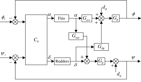
The basic dynamics of the ship motion control system with respect to fins and rudders are shown in Fig. 1. The model has several structural features that can be explored for the integrated fin and rudder roll reduction control system design. The process can be modelled as a TITO (2×2) nonlinear systems (Fig. 1) with a controllerC0, actuators (fins and rudders) are considered as nonlinear subsystems. This is a simple multivariable control system and unlike many integrated fin and rudder stabilization control systems the design of the roll and heading controllers is not separated [4,5]. In classical control scheme, the rolling motion is regulated using fin stabilizers, and the heading is controlled with rudders, involving two single input single output (SISO) systems. A multivariable control scheme will take the system interactions into account, allowing rudders to actively attenuate the roll motion and to control the heading angle which is possible due

Roll Reduction and Course Keeping for the Ship Moving in Waves

with Factorized NGMV Control

(2)

to the separation in the roll and yaw frequency bands. It will also allow the fins to actively reduce the yaw motion and to control the roll angle. In this system, Gφ and Gψ are roll

model and yaw model respectively, dφ and dψ denote the

corresponding wave disturbance time series, φr and ψr are the corresponding input reference signals, respectively. Fin angle signals will be converted to wave slopes by the constant coefficient block Gαw as an input of the ship roll motion model; for the case of roll motion, it is the slope of the waves rather than the wave height that excites the motion, and due to this the roll motion frequency responses are often related to the wave slope rather than the amplitude. In addition, the transfer function Gσφ is a non-minimum phase coupling term, which

complicates the control design and Gαψ is the interaction

from fins to yaw motion. The model details are described in the next sections.

0

C

Fins

Rudders

−

− ₊

+

φ

ψ

r

φ

r

ψ

dφ

d_ψ Gψ

Gδφ

G_αψ

Gφ w

Gα

α

δ

c

α

c

[image:2.612.60.292.271.407.2]

δ

Figure 1. Block diagram of the system

B. Ship Models

The roll-yaw model should be simplified from the 3 DOF nonlinear motions model of Perez [17] by deleting the sway motion equation and nonlinear hydrodynamic items. It will be a linear coupling model if the ship forward speed is set as a constant value. The 2-DOF equations of motions including control forces of fins and rudders are expressed in (1)-(4).

2 (Ix−Kp)p=K Urur +Ku pU p+K Uφuu φ+K pp −ρg GZ∇ φ+mz Ur_G +K_Fα+K_Rδ (1)

(I_z−N_r_) r=N_{u r}U r+N p_p +N_{u p}U p−mx Ur_G

+N_Fα+N_Rδ (2)

φ = p (3)

r

ψ= (4)

where U is the ship speed, ρ is the sea water density, g is the gravity constant, ∇ is the ship volume of displacement, GZis the ship metacentric height, α and δ denote fin and rudder angles. Roll, yaw and their rates are represented by φ, ψ , p

and r , respectively. The subscripts F and R represent stabilizer fins moment and rudder moment, respectively. The coordinate (x_G,y_G,z_G) is the position of the center of gravity in the ship fixed coordinate system.

In order to perform time domain numerical simulations and to derive polynomial models in Fig. 1, we convert motion equations into the following state space model:

x=[ , , , ]p r φ ψ Τ (5) u=[ , ]α δ Τ (6) Using these variables, the state-space model can be written in the standard form,

x=Ax+Bu (7) where the state matrix is

2

0

0 0

0 0 1 0

0 0 0 1

p

u p ur G uu

x p x p x p

p u p u r G

z r z r

K U K K U mz U K U g GZ

I K I K I K

N N U N U mx U

A

I N I N

φ ρ

+

 + − ∇ 

 

− − −

 

 ₊ ₋ 

 

=

 ₋ ₋ 

 

 

  

 

and the input matrix is

0 0

F R

x p x p

F R

z r z r

K K

I K I K

N N

B

I N I N

 

 ₋ ₋ 

 

=  ₋ ₋ 

 

 

 

.

In addition, roll and yaw angle formulas can be described as:

φ =[0, 0,1, 0]x=C xφ (8)

ψ =[0, 0, 0,1]x=C xψ (9)

Hence, the transfer function which from rudder angle to

roll motion 1

(s) / (s) Cφ(sI A) B

φ δ ₌ Τ ₋ −

can be calculated:

2 1

2 2

2

(1 )

( )

( ) (1 )( 2 )

K T s

s

G G

s T s s

δφ φ

φ φ φ

ω φ

δ ξ ω ω

+

= =

+ + + (10)

Base on the above, the rudder-roll interaction block and ship roll motion (i.e. derived by wave slopes) transfer function are:

1 2

(1 )

K T s

G

T s δφ δφ

+ =

+ (11)

and

2

2 2

s 2

Gφ φ

φ φ φ

ω ξ ω ω =

+ + (12)

Similarly, the fin-yaw interaction block Gαψ and ship yaw

motion transfer function G_ψ can be derived in same steps.

C. Disturbance Models

(3)

₂ 2 ₂ ( ) 2

w e

w e e

s

d t

s s

φ

φ φ

ξ ω σ ξ

ξ ω ω

=

+ + (13)

where ξw is the wave damping coefficient and σφ is a constant describing the wave intensity which determined by wave slopes.

In the case of yaw motion, the disturbance is assumed to be of low frequency nature and is modelled by an integrator driven by white noise, described as follow:

d ( )t s

ψ

ψ ψ

σ ξ

= (14)

where σψ is the yaw motion wave strength. ξφ(t) and ξψ(t)

are white noise sequences of unite variance.

III. FACTORIZED NGMVCONTROL

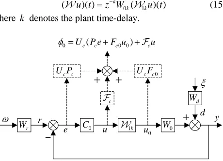
The single DOF factorized NGMV [15,16] is developed by introducing additional control weighting U F_c _c₀ on the output of nonlinear block as shown in Fig. 2.

A. Models and cost index

The nonlinear plant model can be separated into a linear subsystem W_0k and a nonlinear part _1k represents the actuators of the system, the output of the nonlinear system is sometimes referred to as the virtual control input and is denoted u t₀( )=(₁_ku t)( ). It can be written as follows:

( )( ) k ₀ ( ₁ )( ) k k

u t =z W− u t

  (15)

where k denotes the plant time-delay.

0

C _1k W₀

r

W

d

W

0

u u

ω r

ξ

y e

c c

U P U F_c _c₀

c



−

+

0 U P ec( c F uc0 0) cu

φ = + +

[image:3.612.62.292.387.553.2]

d

Figure 2. Single DOF factorised NGMV control system diagram

The plant itself is nonlinear and may have a quite general form (state-space, transfer operators, etc.). However, the reference and disturbance signals are assumed to have linear time invariant (LTI) model representations. This is often valid, since in many applications the models available for the disturbance and reference are LTI approximations. The power spectrum for the combined reference and disturbance signal

( _r _d) _f

f = − =r d W −W ξ=Y ε can be computed as:

*

ff rr dd W Wr r W Wd d

∗

Φ = Φ + Φ = + (16)

where the strictly minimum phase generalized spectral-factor f

Y satisfies Y Yf f*= Φff, * denotes the complex conjugate transpose operate, Wd represents the disturbance shaping

filter as the formulas (13) and (14). For the anti-roll problem, the reference model is a constant set point. ( )ε t is a zero mean white noise and a measurement noise model has not been included to simply the equations.

Assuming the linear disturbance, reference and plant linear subsystem models have the left-coprime polynomial matrix representation:

1

0 0

[W W Wd, r, k] A [C E Bd, r, k]

−

= (17)

then the spectral factor Yf can be written in the polynomial matrix form as Yf A D1 f

−

= .

The signal whose variance is to be minimized is defined: φ₀( )t =U P e tc( c ( )+F u tc₀ ₀( )) (+ cu t)( ) (18) This signal includes a dynamic cost-function weighting polynomial matrix Pc P Pn d1

−

= on the error signal and an input weighting polynomial matrix 1

0 c n d

F =F F− . It also involves a nonlinear control signal costing term (cu t)( ). Typically,

1 ( ) c

P z− is low-pass and F zc( 1)

−

is a constant or a high-pass transfer. The weighting Fc0(z 1)

−

can often be a constant. The all pass matrix 1

20 20

c s

U =L L− is determined from factorized terms involving the cost weightings. The signal variance of

0( )t

φ is to be minimized, so the cost function is: 2

0 { ( )}

J =E φ t (19)

where {}E ⋅ is the expectation operator.

If the plant time-delay is regarded as k, this means the control at time t affects the output k steps later. So the control signal operator can be defined as:

( cu t)( ) z k( cku t)( )

− =

  (20)

(F uc_{0 0})( )t z k(F uc k₀ ₀)( )t

−

= (21)

typically the delay free control weighting operators are assumed invertible.

B. Optimal solution

From Fig. 2, the error signal e= − = − −r y r d W u0 0 , defining the right coprime polynomial matrices Dfa, A0d and

0d

B , Dfb satisfy:

1 1 0d fa f d

A D− =D AP− (22)

1 1

0 0

k

d fb f k d

B D− =z D B F− − (23)

Also, the first term in (18) may be rewritten as:

1

0

( )

c c f n fa d

P r−d =P Y ε=P D A−ε (24) Then the inferred output becomes:

1 1 1

0( )t L L20 20sP D An fa 0d L L20 20s(Fc0 PW uc 0) 0 cu

φ ₌ − −ε₊ − ₋ ₊_

(4)

1 1 1

0 1 1

d k d k

P A B F− − =B A− (26)

Substituting it into the operator and removing the delay times:

1

0 0 ( 1 1)( 1) c k c k n k nk d

PW −F = P B −F A F A − (27)

Now let the matrix PWc 0k−Fc k0 be factorized into strictly minimum phase L1 and non-minimum phase L2 terms. That is the factorized polynomial matrix:

L L₂ ₁=P B_n ₁_k−F A_nk ₁ (28) Given the factor L2 the strictly minimum phase L2s may be introduced that satisfies the relationship: * *

2s 2s 2 2

L L =L L .

Also defining the relationship 1 2 2

c s

U =L L− , then the all pass function can satisfy *

c c

U U =I.

Introducing the following Diophantine equation to expand the first term in (25) into two groups:

₀ ₀ ₂₀ k ₀ ₂₀

d s n fa

F A +L z G− =L P D (29)

According to (24), then the last equation can be written:

1 1 1

20 20 20 0 0 0 k

s c f d

L L− P Y =L F− +z G A− − (30)

Recalling (23) and (29), the first term in the left hand of (25) with time delay can be obtained:

1 1 1 1 1

0 0 20 0 0 20 20 0 0 0

k k k

s f k s d f k

PW =L− F z D B− − +L− L z G A z D B− − − − (31) To obtain an expression for the above operator, introducing the second Diophantine equation:

₀ ₀ ₂₀ k ₀ ₂₀

d s n fb

F B −L z H− =L F D (32)

Combining (23) and (32), the second term in the left hand of (25) with time delay can be obtained,

1 1 1 1 1

0 20 0 0 20 20 0

k k

c s f k s fb d

F L− F z D B− − L− L z H D F− − −

− = − + (33)

Adding (31) and (33), and substituting (22) into this result, then obtaining an implied equation:

1 1 1

0( d fa) 0 0( d fb) 2s 1( d 1)

G P D −W +H F D − =L L F A − (34)

Finally, the k steps ahead of the inferred output signal, involving the weighted error , input and control signals, may therefore be written as:

1

0(t k) L F20 0 (t k)

φ ₊ ₌ − ε ₊

1 1

0 0 1

(G P D( d fa) e (H F D( d fb) k ck) ( ))u t

− −

+ − _ −_ (35)

1 0( d fa)

G P D − 1

ck −



1 0( d fb)

H F D −

1k

W  r

− −

+

d y

[image:4.612.331.554.234.622.2]

Ship + u

Figure 3. Factorised NGMV controller modules

The first term in the right hand of (35) is independent of the control term and the smallest variance is obtained when the remaining terms are zero. Therefore, the control command must satisfy :

1 1 1

0 0 1

( ) _ck ( ( _d _fa) ( ) ( _d _fb) _k ( ))

u t = −− G P D −e t −H F D − u t (36)

so the factorized NGMV controller structure is presented by the Fig. 3.

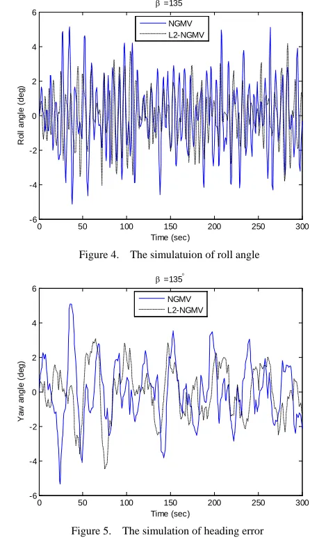
IV. SIMULATION RESULTS

The ship model introduced in reference [17] is a navy vessel with a design forward speed 15 knots and a magnitude constraint for the fins of 25° and the mechanical angle of 40° for rudders (i.e. this vessel is equipped with two rudders). The main objectives are following the tracking of heading set point and the roll reduction. For the sake of convenience, the yaw tracking can be measured using the integral absolute error (IAE) criterion. Similarly, the actuators usage can be measured by integral of absolute their mechanical angles.

0 50 100 150 200 250 300 -6

-4 -2 0 2 4 6

Time (sec)

R

o

ll

an

gl

e (

deg

)

β =135°

NGMV L2-NGMV

Figure 4. The simulatuion of roll angle

0 50 100 150 200 250 300 -6

-4 -2 0 2 4 6

Time (sec)

Y

aw

an

g

le

(d

eg

)

β =135°

NGMV L2-NGMV

Figure 5. The simulation of heading error

In order to evaluate the efficiency of the proposed control scheme for ship anti-roll control in random seas, the roll reduction percentage formula [18] can be used:

Roll Reduction (%) = − ×100

AP RCS AP

(5)

0 50 100 150 200 250 300 -20

-15 -10 -5 0 5 10 15 20

Time (sec)

F

in

an

gl

e

(deg

)

β =135°

NGMV L2-NGMV

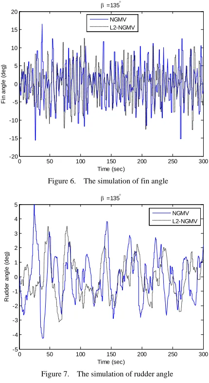
Figure 6. The simulation of fin angle

0 50 100 150 200 250 300 -5

-4 -3 -2 -1 0 1 2 3 4 5

Time (sec)

R

u

dde

r

an

gl

e

(deg

)

β =135°

NGMV L2-NGMV

[image:5.612.80.295.56.450.2]

Figure 7. The simulation of rudder angle

TABLE I. COST VALUE AND PREFORMANCE

No. Comparison of Different Controllers

Control Method Heading Error Roll Reduction

1 NGMV 708.8 90.8

2 Factorised NGMV 637.1 93.1

Control Method Fins Usage Rudders Usage

3 NGMV 2300.0 675.7

4 Factorised NGMV 2177.0 579.6

Using a sea environment described by the ITTC (International Towing Tank Conference) double parameter spectrum with a wave height of 3 m, encounter angleβ = 135° and average wave period of 8 s. The wave damping coefficient ξw and yaw motion wave strength σψ are set as 0.25 and 0.5, respectively. The dynamics of fins and rudders are in the special limiting case where nonlinear actuators revert to pure saturation blocks.

For the purpose of controller design, the continuous time models of system were discretized using the sample time of 1 s. The classical PID controller was discretized and used for the

initial choice of the weighting operators Pc and ck [12]. Assuming the plant is controlled by the nominal PID controller matrix is C z0( 1) diag C

{

φ Cψ

}

− ₌

and with parameters:

1 2

1

1 2

7.2 9.26 2.25 (z )

1 1.05 0.05

z z

C

z z

φ

− −

−

− −

− +

=

− +

1 2

1

1 2

11.1 12.46 2.4 ( )

1 1.05 0.05

z z

C z

z z

ψ

− −

−

− −

− +

=

− +

As assumed in [12], the nominal NGMV design can be based up on these parameters and thus the error weighting

matrix is 1 1

0

( ) ( )

c

P z− =C z− and the control weighting matrix is _ck(z−1)=diag

{

−1 −1

}

. Finally, the added input

weighting is 1

{

}

0 ( ) 1 1

c k

F z− =diag − .

To demonstrate the effectiveness of this proposed method, a series of simulations are performed with the reference input signals φ =r 0 and ψ =r 0° (i.e. the reference signal matrix is

{

0 0

}

r

W =diag ) . Simulation results are shown in Figs. 4-7. Due to the factorized polynomial matrix (27), the factorised NGMV can be simply named as L2-NGMV.

For the roll motion time responses in Fig. 4, the roll reduction ratio of L2-NGMV is a little higher (i.e. 2.3%) than that of NGMV, because their values are both over 90% which is a relatively high performance value. Therefore, the two schemes have a similar effectiveness in terms of roll damping performance. That is also one reason why the fins usage did not have a significant improvement in Fig. 6. In contrast, the yaw motion is significantly further reduced with good speeds of response, shown in Fig. 5. Additionally, the rudder time response results are presented in Fig. 7, the rudder usage is also decreased effectively that will both save driving energy and reduce the mechanical wear of rudder shaft. The values calculated from the cost function are listed in Table I, which indicates the proposed algorithm indeed provide a good performance compare with the normal NGMV method, both in terms motions control and actuators usage. The less improvement in fins usage may be because of the element

Gαψ. The gain of this interaction from fins to yaw motion is

smaller than that from rudder to roll motion, therefore, fins provide the similar moment in the two methods.

By varying the design parameters, it is possible to achieve different of trade-off between required course keeping and roll reduction. Further work will involve including a fully nonlinear multivariable coupling model and an analysis of how the optimal control deals with windup.

V. CONCLUSION

(6)

system. This system is represented by a more complete multivariable coupling form which involved both the interaction from rudders to roll motion and fins to yaw motion. The advantage of this method was to provide better performance and better stability characteristics for the non-minimum phase system under low control costing. In the limiting case when _1k =I (i.e. no constraints in the ship model) and ck→0 , the controller collapses to a version of the standard GMV controller but with weighted output and reference signals in the cost criterion. While the classical NGMV approach will collapses to the standard MV controller in the same case. Using this approach, we have formulated the control problem using a more general form of the NGMV controller. The initial choice of the weighting operators was still based on the classical PID controllers form. Finally, The simulation results were presented to demonstrate the improvement in ship sailing performance.

ACKNOWLEDGMENT

We are grateful for the fund of the China Scholarship Council (CSC) on the joint PhD student project. I also like to appreciate the help of Industrial Control Centre, Department of Electronic and Electrical Engineering, University of Strathclyde on control algorithm.

REFERENCES

[1] T. Perez, M. Blank, “Ship roll damping control,” Annual Reviews in

Control, Vol. 36, pp. 129-147, 2012.

[2] P. Van der Klugt, “Rudder roll stabilization,” Ph.D thesis, Delft University of Technology, Delft, Netherlands, 1987.

[3] T. I. Fossen, Guidance and control of ocean vehicles. New York: John Wiley & Sons, 1994.

[4] F. Alarcin, K. Gulez, “Rudder roll stabilization for fishing vessel using neural network approach,” Ocean Engineering, Vol. 34, pp.1811-1817, 2007.

[5] R. Katebi, “Advanced controller for integrated fin and rudder roll stabilization,” 14th_{Ship Control System Symposium}_{, Ottawa, Canada,} 2009.

[6] J. N. Sgobbo, M. Parsons, “Rudder fin roll stabilization of the USCG WMEC 901 class vessel,” Marine Technology, Vol. 36, pp. 157-170, 1999.

[7] M. T. Sharif, G. N. Roberts, R. Sutton, “Sea-trial experimental results of fin rudder roll stabilization,” Control Engineering Practice, Vol. 3, pp. 703-708, 1995.

[8] M. T. Sharif, G. N. Roberts, R. Sutton, “Final experimental results of full scale fin rudder roll stabilization sea trials,” Control Engineering

Practice, Vol. 4, pp. 377-384, 1996.

[9] G. N. Roberts, M. T. Sharif, R. Sutton, A. Agarwal, “Robust control methodology applied to design a combined steering stabilizer system for warships,” IEEE Proceeding of Control Theory Application, Vol. 144, pp. 128-136, 1997.

[10] M. C. Fang, Y. H. Lin, B. J. Wang, “Applying the PD controller on the roll reduction and track keeping for ship advancing in waves,” Ocean

Engineering, Vol. 54, pp. 13-25, 2012.

[11] M. C. Fang, J. H. Luo, “On the track keeping and roll reduction of the ship in random waves using different sliding mode controllers,” Ocean

Engineering, Vol. 34, pp. 479-488, 2007.

[12] M. J. Grimble, “Design of generalized minimum variance controllers for nonlinear systems,” International Journal of Control Automation

and Systems, Vol. 4, pp. 281-292, 2006.

[13] P. Majecki, R. Katebi, M. J. Grimble, “Rudder roll stabilization with nonlinear GMV control,” International Control Conference, Glasgow, 2006.

[14] M. J. Grimble, P. Majecki, “Polynomial approach to non-linear predictive generalize minimum variance control,” IET Control Theory

and Applications, Vol. 4, pp. 411-424, 2010.

[15] M. J. Grimble, “Factorized NGMV control of nonlinear systems,” Tech.

Report, Industrial Control Center, University of Strathclyde, 2011.

[16] M. J. Grimble, “Factorized H∞ control of nonlinear systems,”

International Journal of Control, Vol. 85, pp. 964-982, 2012.

[17] T. Perez, Ship motion control: Course keeping and roll reduction using

rudder and fins, London: Springer, 2005, pp. 274-279.

[18] M. C. Fang, J. H. Luo, “The ship track keeping with roll reduction using a multiple states PD controller on the rudder operation,” Marine