Model-based fault detection and isolation for wind turbine

(1)

Model-based Fault Detection and Isolation for Wind Turbine

Abdulhamed Hwas* and Reza Katebi**

*

PhD student at University of Strathclyde, Glasgow, UK, email: [email protected]

**

Industrial Control Centre, University of Strathclyde, Glasgow, UK, email: [email protected]

Abstract— In this paper, a quantitative model based method is proposed for early fault detection and diagnosis of wind turbines. The method is based on designing an observer using a model of the system. The observer innovation signal is monitored to detect faults. For application to the wind turbines, a first principles nonlinear model with pitch angle and torque controllers is developed for simulation and then a simplified state space version of the model is derived for design. The fault detection system is designed and optimized to be most sensitive to system faults and least sensitive to system disturbances and noises. A multi-objective optimization method is then employed to solve this dual problem. Simulation results are presented to demonstrate the performance of the proposed method.

Keywords- fault detection; observer; wind turbine; sensor monitoring

I. INTRODUCTION

Faulty components in wind turbine can cause high loses in energy production and possible damage to the wind turbines. The losses may be higher for offshore wind farms. This decreases the reliability and increases the cost of maintenance of the wind turbines. Figure 1 shows the percentage breakdown of the number of failures that occurred during the years 2000-2004 [1]. Most failures were linked to the electrical system followed by sensors and blades/pitch components.

Wind turbine fault monitoring that is a means to avoid abnormal event progression and reduces productivity loss, system breakdowns and damage. It increases safety and reliability of the system to achieve higher performance.

Fault diagnosis methods surveyed in literature can be classified into two general categories, quantitative and qualitative methods. In quantitative method, the understanding is expressed in terms of mathematical functional relationships between the inputs and outputs of the system in the form of system descriptions. In qualitative method, the relationships are expressed in terms of qualitative functions between different components of the system. This approach usually depends upon the knowledge from experts in both the normal and fault cases.

This paper proposes an observer-based Fault Detection and Isolation (FDI) method using a multi-objective optimisation procedure. The paper is organized as follows: Next section is concerned with the requirements for designing an observer and theoretical residual generation. Linear state space model of the wind turbine is presented in section III. Multi-objective optimization genetic algorithm is briefly described in section IV. Fault modelling,

[image:1.612.332.522.232.412.2]

observer-based FDI and simulation results are demonstrated in section V. Finally, the conclusion is drawn in section VI.

Figure 1 The distribution of a number of failures for Swedish wind turbines between 2000-2004 [1]

II. OBSERVER BASED FAULT DETECTION

A. Observer Design

The system described by equation (1) is used to design an observer. The mathematical description of the observer is the same as the system except that the observer has an additional term, the gain K(t), which is continuously correcting the system output and improves the state estimates. The observer is defined in equations (2).

( ) ( ) ( ) ( ) ( ) ( )

x t Ax t Bu t

y t Cx t Du t

= +

ɺ

(1)

ˆ( ) ˆ( ) ( ) ( )[ ( ) ˆ( )] ˆ( ) ˆ( ) ( )

x t Ax t Bu t K t y t y t

y t Cx t Du t

= + +

-= +

ɺ

(2)

where x, u, y are the state, input and output of the system of dimension n, m and r and A, B, C and D are system matrices of appropriate dimensions. Define the difference between

x t

( )

and

x t

ˆ( )

as the state error vector (residual), e(t), thus the dynamic error can be written as:

ˆ

( ) ( ) ( ) ( )

e x tɺ ɺ₌ _-x tɺ ₌ A KC e t_- ₍₃₎ Gears, 9.8

Hub, 0.3

Blades/Pitch , 13.4

Drive, 1.1

Control system, 12.9

Structure, 1.5 yaw System,

6.7 Generator,

5.5 Entire unit, 2.7 Electric System, 17.5 Mechanical

Braks, 1.2 Hydraulics ,

13.3

Sensors, 14.1

(2)

For fault monitroing purposes, a weighted residual is defined as follows:

( ) ( )

r t =QCe t (4)

where Q is residual weighting matrix.

Equation (3) illustrates the dynamic behaviour of the innovation siganl and this is governed by the eigenvalues of the matrix (A-KC). If the matrix A-KC is stable, the error will tend to zero or a constant. If the eigenvalues are chosen in such a way that the dynamic behaviour of the error is asymptotically stable and adequately fast, then any error will tend to zero with sufficient speed. This is possible by choosing an appropriate value for K to achieve the stability, when the system is completely observable [2].

B. Residual Generations

Assume the system is fully observable. The system dynamics with faults and disturbance modelscan be written as:

1

2

( ) ( ) ( ) ( ) ( )

( ) ( ) ( ) ( )

x t Ax t Bu t R f t d t

y t Cx t Du t R f t

= + + +

= + +

ɺ

(5)

where f(t) represents the fault vector and considered to be an unknown function of time. The vector d(t) is the disturbance vector. The matrices R1and R2 are the fault distribution matrices.

Using equation (2) and (5), the estimation error and the residual can be written as:

1 2

( ) ( ) ( ) ( ) ( )

eɺ= A KC e t- +d t +R f t -KR f t ₍₆₎

2 ( ) [ ( ) ( )]

r t =Q Ce t +R f t (7)

Taking Laplace transform of Equation (7) gives: 1

2 1 2

1

( ) [ ( ) ( )]f(s)

( ) [ ( ) (0)]

rf( , , ) ( ) rd( , , )[d(s) e(0)]

r s Q R C sI A KC R KR

QC sI A KC d s e

G s K Q f s G s K Q

-= + - +

-+ - + +

= + +

(8)

where e(0) is the initial value of the state estimation error. The effect of the faults on the signal r(t) can be maximized using the following performance index in frequency domain [3]:

1 2 2 [ , ]

1 1

1 2

( , ) sup {[ (

) ( )] } f

J K Q QR QC j I A

KC R KR

ω ω ω

σ ω

Î

-

-= +

-+

-(9)

where

σ

{.}

denotes the maximal singular value. The disturbance effects on the residual can be minimised using the following performance index:

1

( ) || ( ) ||

d

J K = A KC- - (10)

Sensor, actuator and component fault matrices can be represented as:

1

2 0

0

R

senseor fault

B actuator fault

I component fault

R

I senseor fault

D actuator fault

component fault =

= (11)

Thus we can rewrite fault indices

1 2 2 [ , ]

1

( , ) sup { [ (

) ( )] } af

J K Q Q D QC j I

A KC B KD

ω ω ω

σ ω

Î

-= - +

- +

(12)

1 2 [ , ]

1 1

( , ) sup {[ (

) ( )] } sf

J K Q QI QC j I A

KC KI

ω ω ω

σ ω

Î

-

-= +

-+

-(13)

1 2 [ , ]

1 ( , ) sup { [ ( ) )]}

cf

J K Q QC j I A

KC ω ω ω

σ ω

Î

-= -

-+

(14)

The problem can now be stated as minimising the criteria in (12), (13) and (14) subject to the system dynamics in (5). This is a multi-objective optimisation problem and hence genetic algorithm is proposed to solve the problem.

[image:2.612.314.542.454.685.2]

III. STATE SPACE MODEL OF THE WIND TURBINE Mathematical models for the main components of nonlinear 5MW wind turbine system, particularly aerodynamic, two-mass drive train, DFIG generator and their controllers are developed and validated in previous work [4]. The linear state space matrices for a 5 MW wind turbine defined at wind speed 10 m/s is are follows :

Table I description of parameters of the wind turbine [4]

DESCRIPTION SYMBOL DESCRIPTION SYMBOL

Turbine inertia JT Leakage coefficient

Gearbox ratio ng Stator current id, iq

Generator inertia JG Pitch angle

β

Torsional stiffness Ks Desired pitch angle

β

_d

Torsional damping Cs Mechanical torque Twt

Synchronous speed

ω

_s Electrical torque Te

Stator resistance Rs Control torque c

e

T

Rotor resistance Rr Control rotor voltages vdr ,vqr

Stator inductance Ls Wind turbine speed

ω

_wt

Rotor inductance Ls Generator speed

ω

_m

Mutual inductance Lm

Stator voltage vs

Gearbox ratio ng

(3)

2

1 0 0 0 0 0

1

0 0 1 0 0

0 0 0

0 0 0 ( )

g

S S S

T T T g

S S S

G g G g G g

S

q S m

d m sq r

S m

s s r

n

K C C

J J J n

A K C C

J n J n J n

R i

Lr

i L u R

L L

ω ω σ

ω ω

ω σ

−

 

 

−

 

−

 ₋ 

 

= − 

 

 ₋ 

− −

 

+

 − 

− −

 

 

(15)

1 0 0 0 0 0 0 0 0 0

1

0 0 0 0

1 0 0 0 0

0 0 0 1 0 0 0 0 0 1

T

G

J B

J

 

 

=_ _

−

 

 

(16)

1 0 0 0 0 0

0 0 1 0 0 0

0 0 0 1 0 0

3

0 0 0 0 0 p m s c

r s s

C

n L V K

L L

σ ω

 

 

=

 

−

 

 

(17)

where and Kc=0.8383. D is zeros matrix.

The states x, inputs u and outputs y are defined as: ,

,

The physical variables and parameters are described in table I.

IV. MULTI-OBJECTIVE OPTIMIZATION VIA MULTI OBJECTIVE GENETIC ALGORITHM APPROACH Multi Objective Genetic Algorithm (MOGA) is used to minimise the objective functions. It is more suitable than other approaches such as genetic algorithm because an equality constraint is not required to apply with MOGA [5]. The method finds the solution of problems with two or more objectives to be satisfied all together. Often, such objectives are in conflict with each other, and are expressed in different units. Because of their nature, multi-objective optimization problems normally have not one but a set of solutions, which are called Pareto points or pareto optimal solutions [8].

In order to design the observer, MOGA is used to solve the multi-objective optimization problem defined as follows. Here we need to minimise two objective functions Jsf(K,Q) and Jd(K), with nxm decision variable. Mathematically, the problem can be written as:

Define:

F(X) = [F1(X); F2(X)]

where F1(X)= 1/Jsf(K,Q) and F2(x)=Jd(K), given that max

Jsf(K,Q)= min (1/Jsf(K,Q) and X={x1,……, xnxm} is a vector of decision variables.

The problem is to minimise F(X) subject to: F1j(X) ≤ 0 and F2k(X) ≤ 0.

F1j (X): jth inequality constraint evaluated at X

F2k(X) : kth equality constraint evaluated at X

In the vector function F(x), some of the objectives may be in conflict with others, and some have to be minimized while others are maximized. The constraints define the feasible region X, and any point x∈X is a feasible solution. There is rarely a situation in which all F(X) have an optimum in X at a common point. Therefore, in the absence of preference information, solutions to multi-objective problems are compared using the notion of Pareto dominance.

Without loss of generality, in a minimization problem for all objectives, a solution X1 dominates a solution, X2 if the

two following conditions are true:

• X1 is no worse than X2 in all objectives, i.e., fi(X1) ≤ fi(X2)

• X1 is strictly better than X2 for at least one objective, i.e., fi(X1) < fi(X2).

Then, a solution is said to be Pareto-optimal if it is not dominated by any other possible solution, as described above. Thus, the Pareto-optimal solutions to a multi-objective optimization problem form the Pareto front or Pareto-optimal set [9].

The performance indices Jsf(K,Q) and Jd(K) are functions

in K and Q. Therefore, the parameters set to be designed are the observer gain matrix and residual weighting factor matrix. The matrix K must achieve the stability of the observer and optimisation of the performance indices. Ackermann’s formula is used to parameterize the matrix K [2].

1 2

1 2 1

1 0 0

1

n n n

n n

n

C

CA

K A A A A I

CA

α − α − α α

−

   

   

 

=_ + + + + + _{ }

  

   

   

⋯

⋮ ⋮

(18)

where desired eigenvalues are defined as:

n n n

n n

n s s s s

p s p s p

s− − − = +α +α + +α − +α

− −

1 2

2 1 1 2

1)( ) ( )

( ⋯ ⋯

To improve the design desired eigenvalues are assigned in predefined regions to meet stability and response requirements as in equations[10]:

2

i i i i i

p

=

L

+

(U -L )sin ( ), i=1,...,n

x

Li

≤

pi

≤

Ui

where

Ui=[-6 -10 -1 -3 -8.5 -14]; Li=[-8 -12 -2 -4 -9.5 -20];

where Ui and Li are the lower and higher limits for the

eigenvalues respectively. Index xican be freely selected.

Constrained performance indices have now been transformed T

qr dr m wt

K i i

x=[

β

,

θ

,

ω

,

ω

, , ]

] , , ,

[ _wt _m T_e y= β ω ω

T qr dr c e wt

d

T

v

(4)

into unconstrained as a function of X, where K(x1, x2, x3, x4,

x5, x6) and Q=[x7 x11 x15 x19; x8 x12 x16 x20; x9 x13 x17 x21; x10

x14 x18 x22].

The Matlab Genetic Algorithm Toolbox was utilised. The tuning parameters were set as follows: Initial range of variables= [0; 10000], population size: 75, number of generations: 200.

MOGA solver can accept one or more plot functions through the options argument. This feature is useful for visualizing the performance of the solver at run time. Figure 2(b) is the Pareto front, which plots the Pareto front at every generation. Figure 2(a) is the score diversity for each objective.

From Figure 2, there is only one optimal value on the Pareto front figure, that gives Jsf(K,Q)=infinity and Jd(K) =

258. The eigenvalues at these indices P and matrix K,

residual weighting factor matrix Qare: 0.012 -7.6e-06 3.7e-08 7.3e-10 0.0001 -2. -0.017 -1.8e-14 -0.0003 15.26 -0.016 3.6e-14 0.182 -4338.1 17.35 -2.2e-11 -2.2e-09 1.2e-15 -672 -0.40 -2.2e-09 1.4e-15 11.03 -7.32

K

 

 

= 

 

 

4426 4495 7814 5446 3015 4094 6897 1503 3836 3872 4308 8549 5144 6240 6211 5673

Q

 

 

=

 

[image:4.612.73.292.251.704.2]

 

Fig. 2 Pareto front and the number of individuals for sensor and disturbance performances indices.

V. OBSERVER-BASED SENSOR FDI SCHEME A successful FDI should be accompanied by a fault isolation procedure to isolate a particular fault from others. For example, to determine in which sensor, actuator or component the fault happened. Observer-based residual generator approach is suitable for detecting a fault [6], but to isolate the fault, a method is proposed here as follows..

A. Fault Model

Faults are modelled as unknown change in signals as an additive fault. This fault can be classified according to their source as an actuator

∆

u

(

t

)

, sensor

∆

y

(

t

)

or component

)

(

t

u

_c

∆

faults [3]. Figure 3 shows the effect of additive faults on the observed signals of the inputs and outputs. The component faults affect both the true output and the observed output (

y

_oc). The observed signals for the input and output can be rewritten as below.

( ) ( ) ( ) ( ) o

u t =u t +∆u t +δu t (19)

( ) ( ) ( ) ( )

c

o o c c

y t =u t +∆u t +δu t (20)

0

( ) c( ) ( ) ( ) o

y t=y t +∆y t +δy t (21)

where u t0( ), 0( ) c

y t and y to( )are the actuator, component and sensor outputs respectively.

Fig. 3 A diagram for the additive faults, where δ_{u t}_{( )}and _{( )} c

u t

δ denote the actuator and component disturbance signals respectively. δy t( )is a sensor noise signal.

B. Design of Observer-based Sensor FDI

To design a robust observer-based sensor FDI, we assumed that only one sensor fault occurs, all actuators and components are fault free. Then from equations (5) and (11) the system equation can be expressed as:

2 ( ) ( ) ( ) ( ) ( ) ( ) ( )

x t Ax t Bu t d t

y t Cx t R f t

= + +

= +

ɺ

(22)

Then the residual generator can be created for each sensor as: 2

( ) [( ( ) ( ))( )]

k m k

r t =Q Ce t +R f t C -C (23)

where k is the number of the measurement sensor, Ck is obtained from the matrix C by deleting zero columns and assuming kth row equal zero. Cm is the matrix C without zero columns.

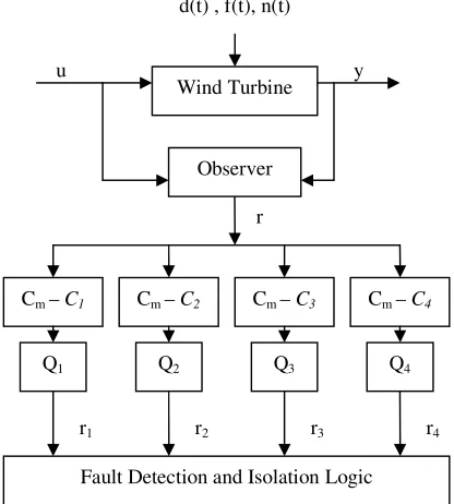
From equation (23), it is obvious that each residual generator is driven making all other residuals equal zero. From above a robust and observer based sensor FDI schemes is designed as shown in figure 4. Each sensor residual (rk) is separated from the output of the residual (r) byr x C

₍

m-Ck

₎

0 50 100 150 200 250 300 0

0.5 1 1.5 2 2.5 3

(a) Score histogram

Score (range)

N

u

m

b

e

r o

f i

n

d

iv

id

u

a

ls

-1 -0.5 0 0.5 1

250 252 254 256 258 260

1/Jsf

Jd

(b) Pareto front 1/Jsf [0 0]

Jd [258.296 258.296]

( )

u t

( )

u t

δ

( )

u t

△

( )

y t

δ

( )

o

u t

( )

y t

∆

0( )

y t

0( ) c

y t

( )

c

u t

δ

( )

c

u t

∆

[image:4.612.329.565.347.450.2]

(5)

, and then dimension of rk is modified using Qk. The advantage of this approach is that it uses only one observer comparing with other approaches, which use a bank of observers such as a structured residual set designed by a dedicated or a generalized observer scheme [6].

For simulation, the values of the residual weighting factors are selected as follows:

1 2

3 10 4

100 1000

Q Q

Q Q Q

= = = = (24)

Q are then obtained using the Method of Multi Objective Genetic Algorithm. Q1, Q2, Q3 and Q4 are residual weighting factors for pitch angle, rotor speed, generator speed and torque sensors, respectively

C. Simulation Results

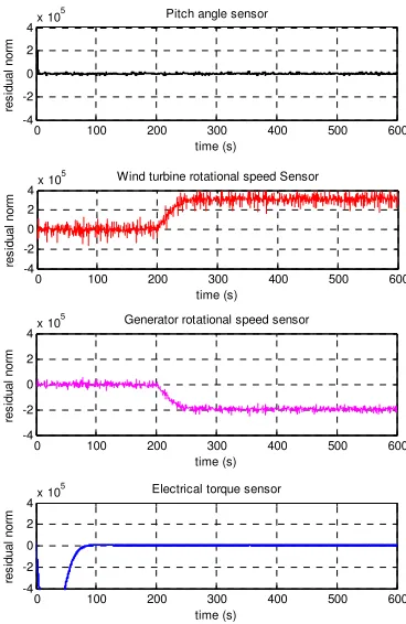
[image:5.612.310.550.90.214.2]

Simulation Results are shown in Figs. 5 to 8. The faults are applied by multiplying the sensor signal by 1.05, i.e. an increase of 5% at 200s, and the transient period is neglected. Fig. 5 shows the residual norm of the pitch sensor increased, when there is a fault. Fig. 6 is for a fault occurred in rotor speed sensor; the residual norm of the rotor and generator rotational speed sensors detects the faults. Fig. 7 for a fault occurred in generator speed sensor and Fig. 8 for a fault occurred in the generator torque sensor. The speed of the fault detection is very fast. Consequently, from figures 5, 6, 7 and 8, we can construct the Boolean decision table as shown in Table II. If a fault occurs, we can compare the results with this fault signature table and decide the location of the fault as shown in the Fig. 4. Therefore, fault detection and isolation are achieved.

Figure 4 A robust sensor FDI scheme. r1, r2, r3 and r4 represent pitch angle, rotor speed, generator speed and generator torque residuals respectively. r contains residuals for all sensors.

For a specific fault, we can now find its location using the following thresholds:

( ) | | ( ) 1 ( ) | | ( ) 0

k k k

r t T f t

> Þ =

£ Þ = (25)

where Tkis the threshold. fk(t) sensor fault. k=1,2 ,3 ,4 (for pitch angle, rotor speed, generator speed and torque sensors). Table II Boolean decision for sensor faults

Residual

Pitch residual

Rotor speed residual

Generator speed residual

Electrical torque residual

Pitch fault 1 0 0 0

Rotor speed

fault 0 1 1 0

Generator

speed fault 0 1 1 1

Electrical

torque fault 0 0 0 1

VI. CONCLUSIONS

A robust observer-based sensor fault detection and isolation scheme is developed for wind turbine. This scheme is systematic and easy to design and implement. Simulation results proved that it is very suitable for detection and isolation faults in sensors and simple to handle multiple faults.

The advantage of the proposed approach is that it depends on only one observer comparing with other approaches, which use a bank of observers such as a structured residual set designed by a dedicated or a generalized observer scheme.

REFERENCES

[1] Johan, R. and B. Lina Margareta, B. Survey of Failures in Wind Power Systems With Focus on Swedish Wind Power Plants During 1997& ndash;2005. Energy Conversion, IEEE Transactions on, 2007. 22(1): p. 167-173.

[2] Ogata, K., (2002). Modern Control Engineering. Pearson Education International, fourth edition.

[3] Chiang, L., Russell, E., and Braatz, R., (2001). Fault Detection and Diagnosis in Industrial Systems. Advanced Textbooks in Control and Signal Processing, Springer.

[4] Hwas, A. (2010). Wind energy conversion system model. Industrial Control Centre, Technical progress report first year, University of Strathclyde.

[5] Hur, Sung-ho and Katebi, M.R. and Taylor, A., (2010). Fault detection and diagnosis of a plastic film extrusion process. In: UKACC International Conference on CONTROL 2010, 2010-09-07 - 2010-09-10, Coventry, UK.

[6] Chen, J. and Patton, R.J., (1999). Robust model-based fault diagnosis for dynamic systems. Kluwer Academic Publishers.

[7] Gertler, J., (1991). Analytical redundancy methods in fault detection and isolation; survey and synthesis, IFAC Fault Detection, Supervision and Safety for Technical Processes, Baden-Baden, Germany, pp. 9–21.

[8] V. Chankong and Haimes, Y. Multi-objective decision making theory and methodology. New York: North-Holland, 1983.

[9] Zeleny, M. Multiple Criteria Decision Making, ser. Quantitative Methods for Management. : McGraw-Hill, 1982

[10] Burrows, S. P. and Patton, R. J. Design of a low sensitivity, minimum norm and structurally constrained control law using eigenstructure assignment. Optimal Control Appl. and Meth., 1991, 12, 131-140. [11] Chen, W., Khan, A., Abid, M. and Ding, S. Integrated design of

observer based fault detection for a class of uncertain nonlinear systems. - Int. J. Applied Mathematics and Computer. Science, 2011, vol.21, no.3

[12] Korbicz, J., Maquin, D. and Theiliol, D. Adances in Control and Fault-Tolerant Systems. Special issue of Int. J. Applied Mathematics and Computer. Science, 2012, vol.22, no.1.

d(t) , f(t), n(t)

Wind Turbine

Cm – C1 Cm – C2 Cm – C3 Cm – C4

Q1 Q2 Q3 Q4

Fault Detection and Isolation Logic

u y

r

r1 r2 r3 r4

[image:5.612.81.289.392.623.2]

(6)

[image:6.612.332.520.86.338.2]

APPENDIX A: SIMULATION RESULTS OF THE ROBUST SENSOR FDI SCHEME.

Fig. 5 Residual norm when a fault occurs in the Pitch angle sensor. _{Fig. 7 Residual norm, when a fault occurs in generator speed sensor.}

0 100 200 300 400 500 600 -4

-2 0 2 4x 10

5 _{Ptch angle sensor}

time (s)

res

id

u

a

l

no

rm

0 100 200 300 400 500 600 -4

-2 0 2 4x 10

5 _{Wind turbine rotational speed Sensor}

time (s)

re

s

id

u

a

l

no

rm

0 100 200 300 400 500 600 -4

-2 0 2 4x 10

5 _{Generator rotational speed sensor}

time (s)

re

s

id

u

a

l

n

o

rm

0 100 200 300 400 500 600 -4

-2 0 2 4x 10

5 _{Electrical torque sensor}

time (s)

re

s

id

ua

l

n

o

rm

0 100 200 300 400 500 600 -4

-2 0 2 4x 10

5 _{Pitch angle sensor}

time (s)

re

s

id

u

a

l

n

o

rm

0 100 200 300 400 500 600 -4

-2 0 2 4x 10

time (s)

re

s

id

u

a

l

n

o

rm

0 100 200 300 400 500 600 -4

-2 0 2 4x 10

time (s)

re

s

id

u

a

l

n

o

rm

0 100 200 300 400 500 600 -4

-2 0 2 4x 10

5 Electrical torque sensor

time (s)

re

s

id

u

a

l

n

o

rm

0 100 200 300 400 500 600 -4

-2 0 2 4x 10

time (s)

re

s

id

u

a

l

n

o

rm

0 100 200 300 400 500 600 -4

-2 0 2 4x 10

5 Wind turbine rotational speed Sensor

time (s)

re

s

id

u

a

l

n

o

rm

0 100 200 300 400 500 600 -4

-2 0 2 4x 10

time (s)

re

s

id

u

a

l

n

o

rm

0 100 200 300 400 500 600 -4

-2 0 2 4x 10

time (s)

re

s

id

u

a

l

n

o

rm

0 100 200 300 400 500 600 -4

-2 0 2 4x 10

time (s)

re

s

id

u

a

l

n

o

rm

0 100 200 300 400 500 600 -4

-2 0 2 4x 10

time (s)

re

s

id

u

a

l

n

o

rm

0 100 200 300 400 500 600 -4

-2 0 2 4x 10

time (s)

re

s

id

u

a

l

n

o

rm

0 100 200 300 400 500 600 -4

-2 0 2 4x 10

time (s)

re

s

id

u

a

l

n

o

[image:6.612.99.262.99.336.2]

rm

[image:6.612.330.521.367.657.2] [image:6.612.86.270.375.658.2]