Grindrod, Peter and Higham, Desmond and Parsons, Mark C. (2012)
Bistability through triadic closure. Internet Mathematics, 8 (4). pp.
402-423. ISSN 1542-7951 , http://dx.doi.org/10.1080/15427951.2012.714718
This version is available at https://strathprints.strath.ac.uk/42969/
Strathprints is designed to allow users to access the research output of the University of Strathclyde. Unless otherwise explicitly stated on the manuscript, Copyright © and Moral Rights for the papers on this site are retained by the individual authors and/or other copyright owners. Please check the manuscript for details of any other licences that may have been applied. You may not engage in further distribution of the material for any profitmaking activities or any commercial gain. You may freely distribute both the url (https://strathprints.strath.ac.uk/) and the content of this paper for research or private study, educational, or not-for-profit purposes without prior permission or charge.
Any correspondence concerning this service should be sent to the Strathprints administrator: [email protected]
The Strathprints institutional repository (https://strathprints.strath.ac.uk) is a digital archive of University of Strathclyde research outputs. It has been developed to disseminate open access research outputs, expose data about those outputs, and enable the
Bistability Through Triadic Closure
Peter Grindrod
∗Desmond J. Higham
†Mark C. Parsons
‡December 12, 2011
Abstract
We propose and analyse a class of evolving network models suitable for de-scribing a dynamic topological structure. Applications include telecommunication, on-line social behaviour and information processing in neuroscience. We model the evolving network as a discrete time Markov chain, and study a very general framework where, conditioned on the current state, edges appear or disappear independently at the next timestep. We show how to exploit symmetries in the microscopic, localized rules in order to obtain conjugate classes of random graphs that simplify analysis and calibration of a model. Further, we develop a mean field theory for describing network evolution. For a simple but realistic scenario incorporating the triadic closure effect that has been empirically observed by so-cial scientists (friends of friends tend to become friends), the mean field theory predicts bistable dynamics, and computational results confirm this prediction. We also discuss the calibration issue for a set of real cell phone data, and find support for a stratified model, where individuals are assigned to one of two distinct groups having different within-group and across-group dynamics.
Keywords calibration, conjugacy, dynamic network, mean field theory, random graph, stochastic process, temporal network, triangulation, voice call data.
1
Preliminaries
A diverse range of application areas give rise to large, complex interaction patterns. In the field of network science, classes of random graph have been proposed and tested as models to capture the structure of these interactions [24]. In many cases, the model may be viewed as an iterative procedure that builds a network sequentially by randomly
∗Department of Mathematics, University of Reading, UK
rewiring an existing structure [25, 30, 31] or by adding nodes and links in order to ‘grow’ a network [3]. In these cases the object of interest, however, is the final, static net-work. Our work differs in that we wish to model a network structure that is inherently dynamic, with edges appearing and disappearing between a fixed set of nodes. Such a scenario arises naturally in many modern, data-rich, applications; for example, telecom-munication (who phoned whom each day), on-line social interaction (who interacted with whom in a chat room), on-line retailing (people who bought this book also bought) [17]. Attention has recently been paid to the issue of extending traditional graph theoretical concepts such as paths to the time-dependent setting [5, 13, 16, 18, 28, 29] and related computational complexity issues [1, 7, 8]. There has also been interest in the waiting times between link changes [2, 32] and the emergence of communities [4, 23]. Also, link
prediction—estimating likely new connections a short time ahead—is being recognized
as an important task [10, 20, 22]. However, in this work we focus on the fundamental issue of modeling and analysing such networks directly and from first principles; that is, prescribing reasonable ‘laws of motion’ and studying the potential behaviors that can arise. Our target applications are digitally generated communication or on-line social interaction networks and our interest lies in the changes of the connectivity structure itself. Related work onadaptive networks [14] has studied scenarios where the nodes are involved in their own dynamical system that is coupled to the dynamic topology—for example, in an epidemiological SIS model, susceptible (S) nodes may seek to avoid links with nodes that are currently infected (I).
The main novel contributions in our work are (a) to introduce the concept of conjugate graphs, which can play an important role in understanding and analysing a model, (b) to derive a mean field theory approach to summarizing long term behaviour, (c) to introduce a simple but realistic nonlinear network evolution model driven by the concept of triadic closure from social science and to show that it admits bistable behaviour, and (d) to consider the issue of model calibration and show that the use of a stratified model improves the fit for a voice call data set.
The presentation is organised as follows. In the next section, we introduce a general stochastic framework and show how modelling and simulation can be simplified by fo-cussing on the dynamics of individual edges. We also illustrate the ideas in the particular case where triadic closure is encouraged—friends of friends tend to become friends. Sec-tion 3 then introduces the concept of conjugacy, which can be used to describe inherent symmetries in a model. A mean field approach is described in section 4 and applied to the triadic closure model in section 5. This model, and a more general stratified version, is fitted to voice call data in section 6, and conclusions are given in section 7.
2
Preliminaries
otherwise, with all aii = 0. Let Sn denote the set of all such adjacency matrices and
let 1 denote the adjacency matrix for the n-vertex clique. If A ∈ Sn then 1−A ∈ Sn
is the adjacency matrix for the complementary graph to that represented by A. Let
Rn denote the set of symmetric n×n real matrices with all elements taking values in
[0,1], with zeros on the main diagonal. So Sn ⊂ Rn. For real n ×n matrices M1 and
M2 the Hadamard (or Schur) product, denoted by M1◦M2, is the matrix obtained by
element-wise multiplication, so that
(M1◦M2)ij = (M1)ij(M2)ij.
If A1, A2 ∈ Sn then A1 ◦A2 ∈ Sn represents the adjacency matrix for the graph of
common edges.
Following the treatment in [12], we use the phrase evolving network model to describe a stochastic rule that generates a sequence of networks represented by a sequence of adjacency matrices, {Ak}Kk=0, where each Ak∈ Sn. We say that Ak represents the state
of the evolving network at the kth time step, tk, where t0 < t1 < . . . < tK are equally
spaced points in time.
It is natural and analytically convenient to focus on Markovian models. We therefore consider the case of afirst order evolving network model characterized by the conditional probability distribution for Ak+1 givenAk, denoted by P(Ak+1|Ak), defined for all pairs
Ak+1, Ak ∈Sn. The expected value of Ak+1 given Ak will be written as
'Ak+1|Ak(:=
!
Ak+1∈Sn
Ak+1P(Ak+1|Ak).
By construction 'Ak+1|Ak( ∈ Rn and the (i, j)th element of 'Ak+1|Ak( contains the
conditional probability that the corresponding edge is present in Ak+1.
We will say that the first order evolving network model,P(Ak+1|Ak), isedge independent
if, givenAk, information about the existence of any particular edges inAk+1 has no effect
on the probability that any other edge is in Ak+1.
We also note that under this assumption of edge independence, any element W ∈ Rn
defines a random graph. The (i, j)th element ofW contains the probability that the cor-responding edge is present and we can construct the associated probability distribution over Sn, say PW(A):
PW(A) = n
"
i=1,j=i+1
(W)(A)ij
ij (1−(W)ij)1
−(A)ij.
For example, if we havep∈(0,1) thenp1∈Rnrepresents a classical Erd¨os-R´enyi/Gilbert
random graph (usually denotedG(n, p)), where each edge exists with independent prob-ability p [24]. Let CL(n,k) ∈ Sn represent the adjacency matrix for a circular lattice on
with every edge present with independent probabilityp, whilepCL(n,k)+q(1−CL(n,k))
is a partial lattice with uniform “short cuts” in the spirit of the classical Watts-Strogatz small world model [25, 31].
In restricting ourselves to first order edge independent evolving network models we may simply consider matrix valued functions
F :Sn→Rn. (1)
Any such mapping F generates a first order edge independent evolving network model for which
< Ak+1|Ak >=F(Ak). (2)
A particularly useful form for F(Ak) is
F(Ak) = (1−ω(Ak))◦Ak+α(Ak)◦(1−Ak), (3)
where α(Ak) and ω(Ak) are given mappings Sn → Rn, representing conditional birth
rates and death rates respectively, as introduced in [12]. It is straightforward to compute a path for such a Markov chain; that is, a particular network sequence whose transitions respect the relevant edge birth and death rates. The following pseudo-code summarizes this approach, given an initial adjacency matrx, A0.
for k = 0,1, 2, ....
Compute α(Ak), ω(Ak)∈Rn
for all disjoint pairs i+=j
if (Ak)ij = 0 then set
(Ak+1)ij = 1 with prob. α(Ak)ij (birth)
(Ak+1)ij = 0 with prob. 1−α(Ak)ij (no change)
else we have (Ak)ij = 1, so set
(Ak+1)ij = 0 with prob. ω(Ak)ij (death)
(Ak+1)ij = 1 with prob. 1−ω(Ak)ij (no change)
end if
end for all pairs
We finish this section by introducing a novel example that fits into this framework. We consider the case where the death rate is a constant for all edges
ω(Ak)≡ω#1, for ω# ∈(0,1), (4)
while the birth rates for edges not present in Ak are given by
α(Ak) = δ1+ǫ1◦A2k, (5)
for some constants δ and ǫ. We assume that 0 < δ ≪1 and, to guarantee probabilities in the range [0,1], that 0< ǫ(n−2)<1−δ.
This model reflects a situation where the more common adjacencies two nonadjacent vertices have in Ak, the more likely they are to become adjacent in Ak+1. In other
words, somebody who is not currently your friend, but who is currently a friend of many of your current friends, has an enhanced chance of becoming your friend at the next step. Forming new associations by the process of triangulating current adjacencies is very natural within a number of applications. In social networks two peers may be likely to become introduced through common friends; in this context, the mechanism is often referred to as triadic closure [11, 19, 27]. In developing cognitive processing capability in the brain, triangulation increases efficiency of communication and resilience, and overabundance of triangles has been observed in both anatomical and functional studies [6, 15, 21].
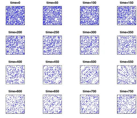
In Figure 1 we show the evolution of a network path from this model withn= 100 nodes and parameter values
#
ω= 0.01, ǫ= 0.0005, δ = 0.0004. (6)
A dot in rowiand column j denotes an edge from nodei to nodej. The initial network was a sample of an Erd¨os-R´enyi graph with expected edge densityp= 0.3—each possible edge exists with independent probability p. The figure shows the adjacency matrix at times tk for k = 50,100,150, . . . ,750. We see that the density of edges increases with
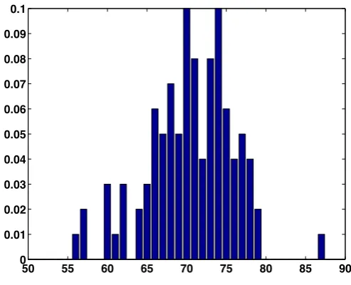
time. Figure 2 gives a histogram of the nodal degrees at the final time, k = 750. The structure appears to be approximately Poisson, and the edge density
$
pk:=
1
n(n−1)/2
! !
i>j(A [k])
ij, (7)
at the final time wasp$750 = 0.712.
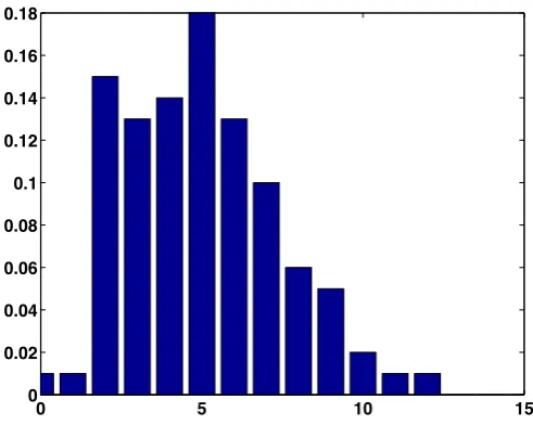
In Figure 3 we repeat the experiment with the same parameter values, but start with an Erd¨os-R´enyi graph with a lower expected edge density of p= 0.15. In this case we see that the edge density decreases over time. The final time value was p$750 = 0.051. The
degree distribution, shown in Figure 4, again appears to be approximately Poisson.
time=0 time=50 time=100 time=150
time=200 time=250 time=300 time=350
time=400 time=450 time=500 time=550
[image:7.595.84.558.222.647.2]time=600 time=650 time=700 time=750
50 55 60 65 70 75 80 85 90 0
[image:8.595.110.357.85.285.2]0.01 0.02 0.03 0.04 0.05 0.06 0.07 0.08 0.09 0.1
Figure 2: Degree distribution for the final network (after 750 iterations) in Figure 1.
3
Classes of Conjugate Random Graphs
In this section we show how symmetries in a model give rise to a natural definition of conjugacy. Assume that the mapping F in (1) characterising a first order edge inde-pendent evolving network is subordinate to a mapping F : Rn → Rn. We will see in
section 4 how this can be rather natural in some examples when we wish to replace Ak
by its own expected value. Let λ denote a (finite or infinite dimensional) parameter ranging over a domain Λ within some suitable space. Let W : Λ→Rn. We will say that
W(λ) is aclass of conjugate random graphs forF if for eachλ∈Λ there exists a unique element g(λ)∈Λ such that
W(g(λ)) =F(W(λ)).
Hence the parameterized set {W(λ)|λ ∈ Λ} ⊂ Rn is positively invariant under F.
Moreover the action of F on Rn can in this case be reduced to the action of g on
Λ.
Suppose thatF :Rn→Rnalso possesses some symmetries. That is, suppose that there
is a subgroup of n×n permutation matrices, H ={Qr}, such that F is invariant under
each of these these permutations; so that
F(A) =QrF(QTrAQr)QTr, A∈Sn, Qr ∈H.
Then F uses no a priori (extra) information about the vertices that distinguishes one permutation in H from another. Now let W ⊂Rn denote the subset of random graphs
inRn that are invariant under the symmetries in H, so that
QT
rW Qr=W,
for all W ∈ W, Qr ∈H. It then follows that
time=0 time=50 time=100 time=150
time=200 time=250 time=300 time=350
time=400 time=450 time=500 time=550
[image:9.595.76.558.230.646.2]time=600 time=650 time=700 time=750
0 5 10 15 0
[image:10.595.111.357.85.287.2]0.02 0.04 0.06 0.08 0.1 0.12 0.14 0.16 0.18
Figure 4: Degree distribution for the final network (after 750 iterations) in Figure 3.
Hence F maps W into W. So, under a suitable parametrization, with some λ ∈Λ, the subset W is a possible class of conjugate random graphs for F.
In the simple case where F is invariant under all possible permutations on n vertices, we know that no subset of nodes is distinguished in any way. For example this will certainly be so whenever F(W) = Q1(W)◦Q2(W) ◦...◦QS(W), where each of the
Qs(W) : Rn →Rn is a polynomial, Qs(W) =β01+β1W +β2W2+...+βµWµ, say, for
suitable nonnegative constants β0, ..., βµ. The random graph W =p1 is invariant under
all such permutations; W is the set of such graphs, parameterized by p ∈ [0,1]. This situation represents a kind of egalitarian or democratic scenario where every node is the same and none is distinguished based on any a priori information. So we must treat all edges and all edge birth dynamics according to the same model.
Alternatively, we may have a stratified model where some extra prior information di-vides the nodes onto two disjoint subsets. (The generalization to a finer partition is immediate.) This could represent a social network between individuals from two sexes for instance, where it was posited that male-male, female-male and female-female in-teractions follow different birth/death dynamics. Similarly, there may be an elite and non-elite (officers and troops), or cultural, or functional splitting of the vertices. To be concrete, suppose that all edges between any of the first n1 vertices satisfy a given
identical dynamic; all edges between any of the lastn2 =n−n1vertices satisfy a distinct
given identical dynamic; and all edges between any of the firstn1 vertices with any of the
last n2 vertices satisfy a third given identical dynamic. Then F will be invariant under
if it has a symmetric block structure: say
(W)ij = 0 if i=j
(W)ij = p if i+=j and i, j ≤n1
(W)ij = q if i+=j and i, j > n1
(W)ij = r if min{i, j} ≤n1 and max{i, j}> n1.
Then W is the set of such graphs, parameterised by three constants: λ = (p, q, r) ∈
[0,1]3 = Λ.
For such a stratified random graph, W ∈ W, the expected number of edges is given by
n1(n1−1)
2 p+
n2(n2−1)
2 q+n1n2r.
We also recall that the Watts-Strogatz clustering coefficient for a node is defined as the ratio of links between the vertices within its neighbourhood divided by the number of links that could possibly exist between them [24, 31]. The expected Watts-Strogatz clustering coefficient then has the form
n1!
2!(n1−3)!p
3+ n2!
2!(n2−3)!q
3+ n1n2!
2!(n2−2)!r
2q+ n2n1!
2!(n1−2)!r
2p+n
1(n1−1)n2pr2+n2(n2−1)n1qr2 n1!
2!(n1−3)!p2+ n2!
2!(n2−3)!q2+ n1n2!
2!(n2−2)!r2+ n2n1!
2!(n1−2)!r2+n1(n1−1)n2pr+n2(n2−1)n1qr
.
This expression has six terms in each of the denominator and the numerator, repre-senting the expected number of open jaws (pairs of edges from a central vertex to two other distinct vertices), and the expected number of those open jaws that are complete triangles, respectively. Six terms arise because the central vertex (of the open jaw) may be in either of the stratified subsets, while the other two vertices may be such that none, one, or both lie within the same subset. The expression simplifies to yield
3(n1−1)n1n2pr2+ 3n1(n2−1)n2qr2+ (n1−2)(n1−1)n1p3+ (n2−2)(n2−1)n2q3)
(2(n1−1)n1n2pr+ 2n1(n2−1)n2qr+ (n1−1)n1n2r2+n1(n2−1)n2r2+ (n1−2)(n1−1)n1p2+ (n2−2)(n2−1)n2q2)
.
In section 6 we compare unstratified and stratified models on voice call data.
4
A Mean Field Approximation for Evolving
Net-works
Our aim in this section is to develop a heuristic approach for analysing the behaviour of an edge independent first order evolving network (2). We begin with the simplifying assumption thatAk has the properties of its own mean (expected) graph, 'Ak|X(, given
In reality of course each of the edges in Ak is there or not, taking a binary value. Hence
by employing the expectation for Ak, the analysis is only an approximation. It will
be particularly poor at times when the probability of edges appearing is relatively small and/or the existence and distribution of just a few edges has a critical effect: they cannot in reality be smeared out.
Alternatively, we may only be given 'Ak|X( ∈ Rn as a random graph itself, conditional
on any previous information X, and we may wish to use our evolving graph model to calculate an estimate for 'Ak+1|X(, and so on. We should calculate
'Ak+1|X(=
!
Ak∈Sn
F(Ak)P(Ak|X).
Instead we might calculate the approximation
'Ak+1|X( ≈ F(
!
Ak∈Sn
AkP(Ak|X)) =F('Ak|X(). (8)
There is equality here if the only nonlinearities in F involve the multiplication of in-dependent stochastic variables. In most cases we will have to consider the expected number(s) of some combinations of edge being present. Here the edge independence assumption is exactly what we need. For example, the expected value of the number of mutual adjacencies (for any give pair of vertices) involves a sum over all pairs of edges connecting to the possible mutual adjacent vertex. These are mutually independent, and of course the two necessary edges within each term are mutually independent. Hence for this type ofF, with each term in the range involving only sums over independent events each of which itself is a product over individual edges, (8) is exact. We refer to (8) as a
mean field approximation for the evolving graph.
Suppose that we may represent < Ak|X >by some random graph, say Wk ∈Rn. Then
using the mean field approximation we simply iterate with F:
Wk′+1 =F(Wk′), k′ =k, k+ 1, k+ 2, . . .
to obtain 'Ak′|X( = Wk′ for all k′ = k, k + 1, k + 2, . . .. This iteration generates a sequence of expected values for the evolving network at all future time steps, given the approximation for Ak, but using the mean field approximation.
Now let us assume that W(λ) is a conjugate random graph for F. If we have Wk =
W(λk), for someλk ∈Λ, then we can iterate with g to produce a sequence
λk′+1 =g(λk′), k′ =k, k+ 1, k+ 2, . . . ,
and it follows that
'Ak′|X(=Wk′ =W(λk′), k ′
=k, k+ 1, k+ 2, . . .
5
Bistability Through Triadic Closure
We now apply this mean field theory to the triadic closure model (4)–(5), where
F(Ak) = (1−#ω)Ak+ (1−Ak)◦(δ1+ǫA2k). (9)
It is easy to see by symmetry of the model (there being no distinguished vertices nor differences in the way vertices and edges are treated) that the Erd¨os-R´enyi graphs are possible conjugate random graphs for this mapping. Substituting 'Ak|X( =pk1 for Ak
as the mean field approximation, we obtain the iteration pk+1 =g(pk) where
g(p) = (1−ω#)p+ (1−p)(δ+ǫ(n−2)p2). (10)
At equilibrium pk+1 =pk≡p⋆, where
p⋆ = (1−p⋆)(δ+ǫ(n−2)p⋆2
)/ω.# (11)
In the limitδ→0, there are three real rootsp⋆if and only if
#
ω < ǫ(n−2)/4. The smallest is δ/(δ+ω#) +O(δ2), representing a sparse graph with almost no triangulation, where
the random birth rate, δ, equilibrates with death rate, ω#; and the the larger roots are at 1/2±%1/4−ω/ǫ# (n−2) +O(δ), where the nonlinear triangulation term equilibrates with the death rate, ω#. Moreover g′
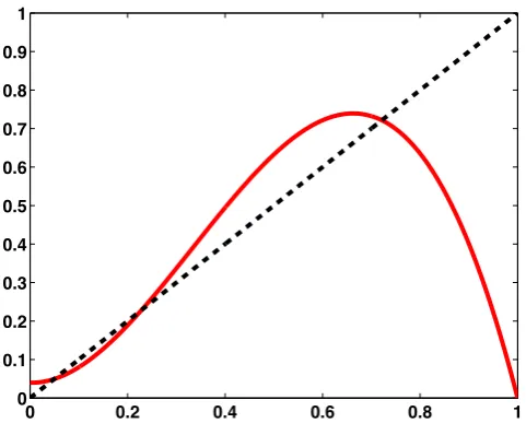
(p) ≥ 0 for all p ∈ [0,1] and g(0) = δ. Hence, in this regime, the two outer steady states are stable for this iteration, whilst the middle root is unstable. Intuitively, with a low initial edge density the triangulation rule cannot get started and the network remains sparse, whereas for a sufficiently high initial edge density, the network evolves into anǫ-dependent state. Figure 5 illustrates the case with
n = 100 and model parameters from (6), where there are stable fixed points at 0.049 and 0.721 surrounding an unstable fixed point atp⋆ = 0.229. These values are consistent
with the experiments in Figures 1–4.
As a further test, Figure 6 shows the results of a single simulation with the same model parameters as in Figure 5. As the initial network, we sampled an Erd¨os-R´enyi random graph with edge probability p = 0.3. The jagged curve in the figure shows the edge density (7) against tk. The solid curve represents the mean field recurrence from (10),
with p0 = 0.3. We see that there is very good agreement when this macroscopic
quan-tity is computed directly from the full microscopic simulation and from the mean field approximation.
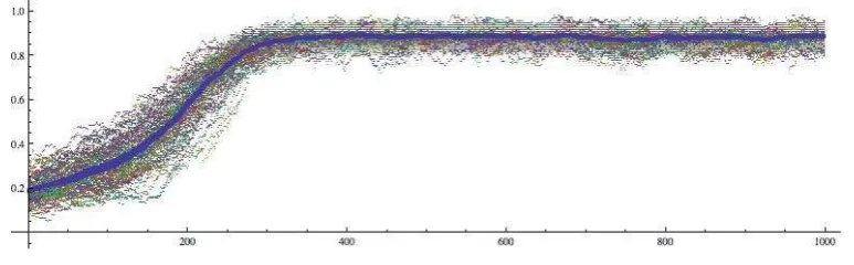
Our mean field analysis predicts that the long term behaviour may be sensitive not only to the initial conditions but also to the transient stochastic fluctuations. Figure 7 confirms this effect by showing five separate simulations with the same model parameters, all starting out from the same graph, a sample of an Erd¨os-R´enyi graph with edge probability
p = 0.23. This value was chosen deliberately to be close to the unstable middle fixed point of the mean field equation. As in Figure 6, we plot the edge densityp$kat each time
0 0.2 0.4 0.6 0.8 1 0
[image:14.595.185.426.85.284.2]0.1 0.2 0.3 0.4 0.5 0.6 0.7 0.8 0.9 1
Figure 5: Graph of p(dashed) and (1−p)(δ+ǫ(n−2)p2)/
#
[image:14.595.178.440.363.538.2]ω (solid): the fixed points are at 0.049, 0.229 and 0.721. (Here n = 100 and parameter values are taken from (6).)
Figure 6: Comparison of p$k in (7) estimated from a simulation with solution to the
dynamical mean field equation (10).
At eachtk, we can calculate the average Watts-Strogatz clustering coefficient,Ck, defined
as the clustering coefficient averaged over all nodes. It is interesting to compare its evolution with that of the edge density, p$k. Since the initial network and long term
networks are Erd¨os-R´enyi graphs we will have have Ck = p$k there. For the simulation
in Figure 8, we see that Ck increases slightly ahead of p$k, as initially random clusters
strengthen, before they infill at the higher density. The individual, vertex-wise, values of the clustering coefficient increase in variance during the phase of rapid growth; see Figure 9.
Figure 7: Five simulations starting from the same network: we show the fraction of edges p$k in (10) at each time step (equivalent to the edge probability p for an evolving
[image:15.595.174.442.365.543.2]Erd¨os-R´enyi random graph).
Figure 8: Ratio of average clustering coefficient to edge density: Ck/p$k.
Figure 9: Vertex-level clustering coefficients as the network in Figure 8 evolves.
[image:15.595.114.501.577.697.2]service provider may wish to stimulate early activity to move the edge density into a region where the network will then self-organise into a profitable, well connected regime.
6
Application to Voice Call Data
In this section we consider an evolving network data set of pairwise mobile phone com-munications during a period of the year where connections were on the increase. We compare the unstratified (homogeneous) model and a stratified model introduced in sec-tion 3, by first calibrating them via the evolusec-tion of the appropriate edge densities, and then examining how they predict the corresponding possible evolution of the average Watts-Strogatz clustering coefficient.
Suppose that we observe an evolving random graph. By making an assumption aboutF, and selecting an appropriate subgroup of permutations,Q, we may derive the mean field equations, over W, which will involve the dynamical parameters from F. From data we can calculate the evolution of the coordinates λ describing W. By fitting these to the mean field model we can estimate the unknown dynamical parameters. Then the choice of model may be validated or invalidated by checking other evolving network metrics not used to do the calibration.
For example here we consider weeks 8 through 15 of data from the Reality Mining data set given in [9], showing voice call between around 150 people over time. We consider the weekly call networks, summarizing which pairs of people communicated during successive weeks.
Assuming initially that no people are distinctive in any way, we first fit the simple three parameter unstratified model in (9). Assuming a homogeneous population, since F is invariant under all permutations, the mean field dynamics act overW ={p1|p∈[0,1]}. So, as described in section 5 we have pk+1 = g(pk) for g in (10). From the data we can
estimate pk viap$k in (7) , the density of edges present. We have
$
pk+1 = (1−ω#)p$k+ (1−p$k)(δ+ǫ(n−2)p$2k) + errk,
where the errors, errk, arise as an average over n(n−1)/2 independent edge-processes
each of which must take binary values. Thus a Gaussian approximation to the structure of the errors is reasonable and the parameters may be fitted with simple least squares. This results in estimates (δ, ǫ,ω#) = (0.02170,0.00868,0.18399). In Figure 10 we showp$k
as well as the 5th and 95th percentiles arising from 200 simulations with the full model, each starting out from A8 and using the estimated dynamical parameters. We see that
the calibrated model provides an ensemble of simulations about the actual data.
Now let us examine the performance of the model by considering the evolution of the average Watts-Strogatz clustering coefficient,Ck, from week to week. For an Erd¨os-R´enyi
8 9 10 11 12 13 14 15 0.04
0.05 0.06 0.07 0.08 0.09 0.1 0.11 0.12 0.13 0.14
[image:17.595.183.428.78.283.2]Edge Density
Figure 10: Evolution of edge density by week from data (crosses), and also the 5 and 95 percentile values (triangles) achieved via an ensemble of model simulations each using the fitted dynamical parameter values, and each starting from A8.
8 9 10 11 12 13 14 15
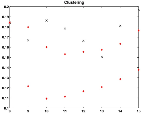
0.1 0.11 0.12 0.13 0.14 0.15 0.16 0.17 0.18 0.19 0.2
Clustering
Figure 11: Evolution of Ck by week from data (crosses), and also the the 5 and 95
percentile values (triangles) achieved via an ensemble of model simulations each using the fitted dynamical parameter values, and each starting from A8.
poorly since the observed values forCk are much higher than those achievable under the
[image:17.595.182.428.435.638.2]8 9 10 11 12 13 14 15 0.04
0.05 0.06 0.07 0.08 0.09 0.1 0.11 0.12 0.13
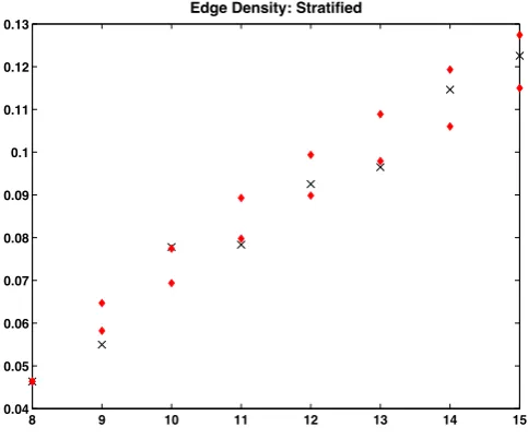
[image:18.595.184.426.80.281.2]Edge Density: Stratified
Figure 12: Evolution of edge density by week from data (crosses), and also the 5 and 95 percentile values (triangles) achieved via an ensemble of model simulations each using the fitted dynamical parameter values, and each starting from A8.
One explanation for this poor fit is that the population is not homogeneous, which motivates us to consider a stratified random graph model of the type introduced in section 3, in order to increase the clustering within some subgroup, and thus increase the values forCk overall, while keeping the overall edge density low. We partitioned the
vertices into two sets; one of sizen1 = 92, and one of sizen2 = 14. This was done by first
clustering the vertices using the sum of the adjacency matrices as a similarity matrix and adopting a Fiedler vector approach to give a spectral clustering [12, 26]. In other applications this task might be done a priori on grounds such as gender, functional role or responsibility of the individuals.
Assuming an identical birth and death dynamic for edges within each vertex subset and between the subsets, then, in the (p, q, r) notation of section 3, the mean field dynamic at the (k+ 1)th time step becomes
pk+1 = (1−ω#p)pk+ (1−pk)(δp +ǫp((n1−2)pk2 +n2r2k)),
rk+1 = (1−ω#r)rk+ (1−rk)(δr+ǫr((n1−1)pkrk+ (n2 −1)qkrk)),
qk+1 = (1−ω#q)qk+ (1−qk)(δq+ǫq((n2−2)qk2+n1r 2)),
involving nine parameters. These nine degrees of freedom can be fitted using the es-timates for (pk, qk, rk). We obtain the overall edge density evolution shown in Figure
12.
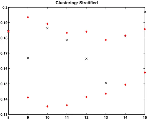
Again let us examine the performance of the stratified model by considering the evolution of the Watts-Strogatz clustering coefficient, Ck. In Figure 13 we see that the model
8 9 10 11 12 13 14 15 0.13
0.14 0.15 0.16 0.17 0.18 0.19 0.2
[image:19.595.185.429.187.391.2]Clustering: Stratified
Figure 13: Evolution ofCk by week from data (crosses), and also the 5 and 95 percentile
values (triangles) achieved via an ensemble of stratified model simulations each using the fitted dynamical parameter values, and each starting from A8.
7
Discussion
The motivation for this work was to develop a framework for modelling and analysing dynamic connectivity structures. A successful model offers the potential to illustrate the range of possible behaviors and also to allow predictions under various ‘what if’ scenarios, such as spiking information (rumours, marketing, stimulus) or making direct perturbations (disabling or enhancing specific vertices or edges).
By introducing the concept of conjugate graphs and developing a mean field theory, we opened up the potential to approximate and calibrate the dynamics of observed networks. In particular, this can help us to identify when the network is close to an unstable rest point, where stochastic details will be important.
for many other classes of evolving network mechanisms to be proposed, analysed and calibrated using the ideas and tools developed here.
Acknowledgment
The authors would like to thank the Engineering and Physical Sciences Research Coun-cil and the Research CounCoun-cils UK Digital Economy programme for support through the MOLTEN (Mathematics Of Large Technological Evolving Networks) project, EP/I016058/1 and HORIZON, EP/G065802/1.
References
[1] C. Avin, M. Kouck´y, and Z. Lotker, How to explore a fast-changing world
(cover time of a simple random walk on evolving graphs), in ICALP ’08: Proceedings
of the 35th international colloquium on Automata, Languages and Programming, Part I, Berlin, Heidelberg, 2008, Springer-Verlag, pp. 121–132.
[2] A.-L. Barab´asi,The origin of bursts and heavy tails in human dynamics, Nature, 435 (2005), pp. 207–211.
[3] A.-L. Barab´asi and R. Albert,Emergence of scaling in random networks, Sci-ence, 286 (1999), pp. 509–12.
[4] D. S. Bassett, N. F. Wymbs, M. A. Porter, P. J. Mucha, J. M. Carlson, and S. T. Grafton, Dynamic reconfiguration of human brain networks during
learning, Proc. Nat. Acad. Sci., 108 (2011), p. doi: 10.1073/pnas.1018985108.
[5] K. Berman, Vulnerability of scheduled networks and a generalization of Menger’s
Theorem, Networks, 28 (1996), pp. 125–134.
[6] E. Bullmore and O. Sporns, Complex brain networks: graph theoretical
anal-ysis of structural and functional systems, Nature Reviews Neuroscience, 10 (2009),
pp. 186–198.
[7] A. E. Clementi, C. Macci, A. Monti, F. Pasquale, and R. Silvestri,
Flooding time in edge-Markovian dynamic graphs, in Proceedings of the 27th
An-nual ACM SIGACT-SIGOPS Symposium on Principles of Distributed Computing (PODC’08), ACM Press, 2008, pp. 213–222.
[8] A. E. F. Clementi, F. Pasquale, A. Monti, and R. Silvestri,Information
spreading in stationary Markovian evolving graphs, in Proceedings of the 2009 IEEE
[9] N. Eagle, A. S. Pentland, and D. Lazer,Inferring friendship network
struc-ture by using mobile phone data, Proceedings of the National Academy of Sciences,
106 (2009), pp. 15274–15278.
[10] P. Esfandiar, F. Bonchi, D. Gleich, C. Greif, L. Lakshmanan, and B.-W. On, Fast Katz and commuters: Efficient estimation of social relatedness
in large networks, in Algorithms and Models for the Web-Graph, R. Kumar and
D. Sivakumar, eds., vol. 6516 of Lecture Notes in Computer Science, Springer Berlin/Heidelberg, 2010, pp. 132–145.
[11] S. Goodreau, J. A. Kitts, and M. Morris, Birds of a feather or friend of a friend? Using exponential random graph models to investigate adolescent friendship
networks, Demography, 46 (2009), pp. 103–126.
[12] P. Grindrod and D. J. Higham, Evolving graphs: Dynamical models, inverse
problems and propagation, Proceedings of the Royal Society, Series A, 466 (2010),
pp. 753–770.
[13] P. Grindrod, M. C. Parsons, D. J. Higham, and E. Estrada,
Communi-cability across evolving networks, Phys. Rev. E, 83 (2011), p. 046120.
[14] T. Gross and B. Blasius,Adaptive coevolutionary networks: a review, J. Royal Society Interface, 5 (2008), pp. 259–71.
[15] Y. He, Z. J. Chen, and A. C. Evans, Small-world anatomical networks in the
human brain revealed by cortical thickness from MRI, Cerebral Cortex, 17 (2007),
pp. 2407–2419.
[16] P. Holme, Network reachability of real-world contact sequences, Physical Review E, 71 (2005).
[17] P. Holme and J. Saram¨aki, Temporal Networks, ArXiv e-prints, (2011).
[18] G. Kossinets, J. Kleinberg, and D. Watts, The structure of information
pathways in a social communication network, in Proceeding of the 14th ACM
SIGKDD international conference on Knowledge discovery and data mining, KDD ’08, New York, NY, USA, 2008, ACM, pp. 435–443.
[19] G. Kossinets and D. J. Watts,Empirical analysis of an evolving social network, Science, 311 (2006), pp. 88–90.
[20] D. Liben-Nowell and J. Kleinberg, The link-prediction problem for social
networks, Journal of the American Society for Information Science and Technology,
58 (2007), pp. 1019–1031.
[22] Z. Lu, B. Savas, W. Tang, and I. Dhillon, Supervised link prediction using
multiple sources, in Data Mining (ICDM), 2010 IEEE 10th International Conference
on, Dec. 2010, pp. 923 –928.
[23] P. J. Mucha, T. Richardson, K. Macon, M. A. Porter, and J.-P.
On-nela, Community structure in time-dependent, multiscale, and multiplex networks,
Science, 328 (2010), pp. 876–878.
[24] M. E. J. Newman, Networks: An Introduction, Oxford Univerity Press, Oxford, 2010.
[25] M. E. J. Newman, C. Moore, and D. J. Watts, Mean-field solution of the
small-world network model, Physical Review Letters, 84 (2000), pp. 3201–3204.
[26] G. Strang, Computational Science and Engineering, Wellesley-Cambridge Press, 2008.
[27] M. Szell and S. Thurner,Measuring social dynamics in a massive multiplayer
online game, Social Networks, 39 (2010), pp. 313–329.
[28] J. Tang, M. Musolesi, C. Mascolo, V. Latora, and V. Nicosia,Analysing
information flows and key mediators through temporal centrality metrics, in SNS ’10:
Proceedings of the 3rd Workshop on Social Network Systems, New York, NY, USA, 2010, ACM, pp. 1–6.
[29] J. Tang, S. Scellato, M. Musolesi, C. Mascolo, and V. Latora,
Small-world behavior in time-varying graphs, Physical Review E, 81 (2010), p. 05510.
[30] A. Wagner, How the global structure of protein interaction networks evolves, Pro-ceedings of The Royal Society of London. Series B, Biological Sciences, 270 (2003), pp. 457–466.
[31] D. J. Watts and S. H. Strogatz,Collective dynamics of ‘small-world’ networks, Nature, 393 (1998), pp. 440–442.
[32] K. Zhao, J. Stehl´e, G. Bianconi, and A. Barrat, Social network dynamics