City, University of London Institutional Repository
Citation
: Karcanias, N. & Halikias, G. (2011). Approximate zero polynomials of polynomial
matrices and linear systems. 2011 50th IEEE Conference on Decision and Control and
European Control Conference, pp. 465-470. doi: 10.1109/CDC.2011.6160302
This is the accepted version of the paper.
This version of the publication may differ from the final published
version.
Permanent repository link:
http://openaccess.city.ac.uk/7297/
Link to published version
: http://dx.doi.org/10.1109/CDC.2011.6160302
Copyright and reuse:
City Research Online aims to make research
outputs of City, University of London available to a wider audience.
Copyright and Moral Rights remain with the author(s) and/or copyright
holders. URLs from City Research Online may be freely distributed and
linked to.
Approximate Zero Polynomials of Polynomial Matrices and Linear
Systems
Nicos Karcanias and George Halikias
Abstract— This paper introduces the notions of approximate and optimal approximate zero polynomial of a polynomial matrix by deploying recent results on the approximate GCD of a set of polynomials [1] and the exterior algebra [4] representation of polynomial matrices. The results provide a new definition for the “approximate”, or “almost” zeros of polynomial matrices and provide the means for computing the distance from non-coprimeness of a polynomial matrix. The computational framework is expressed as a distance problem in a projective space. The general framework defined for polynomial matrices provides a new characterization of approximate zeros and decoupling zeros [2], [4] of linear systems and a process leading to computation of their optimal versions. The use of restriction pencils provides the means for defining the distance of state feedback (output injection) orbits from uncontrollable (unobservable) families of systems, as well as the invariant versions of the “approximate decoupling polynomials”.
I. INTRODUCTION
The notion of almost zeros and almost decoupling zeros for a linear system has been introduced in [4] and their prop-erties have been linked to mobility of poles under compensa-tion. The basis of that definition has been the representation of the Pl¨ucker embedding by using the Grassmann polyno-mial vectors [3]. This process has introduced new system invariant and led to the definition of “almost zeros” of a set of polynomials as the minima of a function associated with the polynomial vector [2]. Here we develop the concept further by introducing the notion of “approximate zero polynomials” using the exterior algebra framework introduced in [4], and then by deploying the results on the approximate GCD defined in [1]. The notion of “approximate zero polynomials” (AZP) of a polynomial matrix and “optimal” AZP are defined in terms of an optimization expressing the computation of the distance of a point in a projective space from the intersection of two varieties. The first is the Grassmann variety [3], [13] and the second is the given degree GCD variety of the projective space. The results on polynomial matrices are then used to define the “approximate input, output decoupling zero polynomials” and “approximate zero polynomial” of a linear system.
Defining the distance of a system described by the pair
(A,B) (pair (A,C)) from the family of uncontrollable (un-observable) systems has been a subject under consideration
N. Karcanias is with the Systems and Control Research Centre, School of Engineering and Mathematical Sciences, City University, Northampton
Square, London EC1V 0HB, [email protected]
G. Halikias is with the the Systems and Control Research Centre, School of Engineering and Mathematical Sciences, City University, Northampton
Square, London EC1V 0HB, [email protected]
for some time [15]. It is worth pointing that although the controllability (observability) properties are invariant under state feedback (output injection), their “strength” (measured with different criteria) is not. This raises the question of whether invariant measures can be defined. Here we intro-duce a new framework for evaluating such distances that allows the computation of the specific system(A,B)((A,C)), as well as the state feedback (output injection) orbits (A+ BL,B)((A+KC,C)) from the uncontrollable (unobservable) systems. The latter is a new dimension to the problem and it is complemented by the definition of the corresponding decoupling zero polynomials.
We are using the exterior algebra framework by deploying the Pl¨ucker embedding [3] to associate polynomial vectors to polynomial matrices; thus we have a framework that allows a proper definition of the notion of “approximate matrix divisor” of polynomial models, as well as the notion of the distance of a polynomial matrix from families of non-coprime matrices. It is shown that the characterisation and computation of an “approximate matrix divisor” is equivalent to a distance problem of a general set of polynomials from the intersection of two varieties, a GCD (defined by the degree of the desirable GCD) and the dynamic Grassmann variety that is defined by the Forney order [8] of the polynomial matrix. The notion of approximate matrix divisor introduced here refers to a family of square matrices all having the same polynomial as determinant.
II. DEFINITIONS AND PRELIMINARY RESULTS
Consider the linear system S(A,B,C,D) :
S(A,B,C,D): ˙x=Ax+Bu, y=Cx+Du (1)
whereA∈Rn×n,B∈Rn×p,C∈Rm×n andD∈Rm×p. It is assumed that(A,B)is controllable and(A,C)is observable. Alternatively,S(A,B,C,D)is defined by the transfer function matrix represented in terms of left, right coprime matrix fraction descriptions (LCMFD, RCMFD), as
G(s) =Dl(s)−1Nl(s) =Nr(s)Dr(s)−1 (2)
whereNl(s),Nr(s)∈Rm×p[s],Dl(s)∈Rm×m[s] andDr(s)∈
Rp×p[s]. We shall denote by N a left annihilator of B, i.e.
N∈R(n−p)×n,NB=0 and byM a right annihilator ofC, i.e.
M∈Rn×(n−m),CM=0, whereN,M have full rank.
The family of frequency assignment problems has a com-mon formulation that allows a unifying treatment in terms of the Abstract Determinantal Assignment Problem. Thus :
(i) Pole assignment by state feedback:Pole assignment by state feedbackL∈Rn×preduces to
pL(s) =det{sI−A−BL}=det{B(s)L˜} (3)
whereB(s) = [sI−A,−B]is defined as the system controlla-bility pencil and ˜L= [In,Lt]t. The zeros ofB(s)are the input
decoupling zeros of the system [6].
(ii) Design observers: The design of an n-state observer by an output injectionT ∈Rn×m reduces to
pT(s) =det{sI−A−TC}=det{TC(s)˜ } (4)
whereC(s) = [sI−At,−Ct]t is the observability pencil and ˜
T = [In,T] represents output injection. The zeros of C(s)
define the output decoupling zeros [6].
(iii) Zero assignment by squaring down:Given a system withm>pandc∈Rpthe vector of the variables which are to be controlled, thenc=HywhereH∈Rp×m is asquaring down post-compensator, and G′(s) =HG(s) is the squared down transfer function matrix [5]. A right MFD for G′(s)
is defined G′(s) = HNr(s)Dr(s)−1, G(s) = Nr(s)Dr(s)−1.
FindingH such thatG′(s) has assigned zeros is defined as thezero assignment by squaring down problem [5], and the zero polynomial ofS(A,B,HC,HD)is
zK(s) =det{HNr(s)} (5)
Remark 1:The zeros ofM(s)are fixed zeros of all polyno-mial combinants f(s). The input (output) decoupling zeros are fixed zeros under state feedback (output injection) and nonsquare zeros are fixed zeros under all squaring down compensators. For the case of polynomial matrices, the zeros are expressed as zeros of matrix divisors [7], or as the roots of the GCD of a polynomial multi-vector [3], [4]. The latter formulation allows the development of a framework for defining “almost zeros” in a way that also permits the quantification of the strength of approximation.
A. The Abstract Determinantal Assignment Problem (DAP):
This problem is to solve equation (7) below with respect to the constant matrixH:
det(HN(s)) =f(s) (6)
where f(s) is the polynomial of an appropriate d-degree. DAP is a multilinear nature problem of a determinantal character. IfM(s)∈Rp×r[s],r≤psuch that rank{M(s)}=r
and letH be a family of full rank r×p constant matrices having a certain structure then DAP is reduced to solve equation (7) with respect toH∈H
fM(s,H) =det(HM(s)) =f(s) (7)
where f(s)is a real polynomial of some degreed.
Notation [3]: Let Qk,n be the set of lexicographically
ordered, strictly increasing sequences of k integers from 1,2, . . . ,n. If{xi
1, . . . ,xik}is a set of vectors of a vector space
V, ω= (i1, ...,ik)∈Qk,n, then xi1∧. . .∧xik=xω∧ denotes
the exterior product and by∧rV we denote ther-th exterior power ofV. IfH∈Fm×nandr≤min{m,n}, then byCr(H)
we denote ther-th compound matrix ofH [3].
Ifhti,mi(s),i∈r, denote the rows of H, columns of M(s)
respectively, then
Cr(H) =ht1∧. . .∧htr=ht∧ ∈Rl×σ (8)
Cr(M(s)) =m1(s)∧. . .∧mr(s) =m∧ ∈Rσ[s],σ=
( p r )
(9)
and by Binet-Cauchy theorem [3] we have that [4]:
fM(s,H) =Cr(H)Cr(M(s)) =⟨h∧,m(s)∧⟩=
∑
ω∈Qr,p
hωmω(s)
ω= (i1, . . . ,ir)∈Qr,p, andhω,mω(s)are the coordinates of
h∧, m(s)∧, respectively. Note thathω is ther×r minor of
H which corresponds to the ω set of columns ofH andhω
is a multilinear function of the entrieshi j ofH.
DAP Linear sub-problem: Setm(s)∧p(s)∈Rσ[s], f(s)∈
R[s]. Determine the existence ofk∈Rσ,k̸=0, such that
fM(s,H) =ktp(s) =
∑
kipi(s) =f(s), i∈σ (10)DAP Multilinear sub-problem: Assume that K is the family of solution vectorskof (5). Determine if there exists
Ht= [h1, ...,hr],Ht∈Rp×r, such that
h1∧. . .∧hr=h∧=k, k∈K (11) Lemma 1 [3]: Let k ∈Rσ, σ =(pr) and let kω, ω = (i1, ...,ir)∈Qr,p be the Pl¨ucker coordinates of a point in
Pσ−1(R). Necessary and sufficient condition for the existence
ofH∈Rr×p,H= [h1, . . . ,hr]t, such that
h∧=h1∧. . .∧hr=k= [. . . ,kω, . . .]t (12) is that the coordinateskω satisfy the quadratics
r+1
∑
k=1
(−1)v−1ki
1,...,ir−1,jkvj1,...,jv−1,jv+1,jr+1=0 (13) where 1≤i1<i2< . . . <ir−1≤n, 1≤j1<j2< . . . <jr+1≤
The quadratics defined by equation (13) are known as the
Quadratic Pl¨ucker Relations (QPR) [3] and they define the Grassmann varietyΩ(r,p)of Pσ−1(R).
III. GRASSMANN INVARIANTS OF LINEAR SYSTEMS
Consider T(s)∈ Rp×r[s], T(s) = [t1(s), . . . ,tr(s)], p ≥ r, rank{T(s)} = r, Xt = RangeR(s)(T(s)). If T(s) =
M(s)D(s)−1is a RCMFD ofT(s), thenM(s)is a polynomial basis for Xt. If Q(s) is a greatest right divisor of M(s)
thenT(s) =M(s)Q(s)D(s)˜ −1, where ˜M(s) is a least degree polynomial basis of Xt [7]. A Grassmann Representative
(GR) for Xt is defined by [4]
t(s)∧=t1(s)∧. . .∧tr(s) =m˜1(s)∧. . .∧m˜r(s)·zt(s)/pt(s)
(14) where zt(s) =det{Q(s)}, pt(s) =det{D(s)} are the zero,
pole polynomials of T(s) and ˜m(s) =m1(s)∧. . .∧m˜r(s)∈
Rσ[s], σ =(p r
)
, is also a GR of Xt. Since ˜M(s) is a least
degree polynomial basis for Xt, the polynomials of ˜m(s)∧
are coprime and ˜m(s)∧ is a reduced polynomial GR (R -R[s]- GR) ofXt. Ifδ =deg{m(s)˜ ∧}, then δ is the Forney
dynamical order [8] of Xt. ˜m(s)∧may be expressed as
˜
m(s)∧=p(s) =p0+p1s+. . .+pδsδ =Pδ·eδ(s) (15) where Pδ ∈Rσ×(δ+1) is a basis matrix for ˜m(s)∧ and
eδ(s) = [1,s, ...,sδ]t. All R[s]-GRs of Xt differ only by a
nonzero scalar factora∈Rand if ∥pδ∥=1, we define the canonical R[s]-GR g(Xt) and the basis matrix Pδ is the
Pl¨ucker matrix ofXt [4].
Theorem 1: g(Xt), or the associated Pl¨ucker matrix Pδ,
is a complete (basis free) invariant of Xt.
IfM(s)∈Rp×r[s],p≥r, rank{M(s)}=r, is a polynomial basis of Xt, then M(s) =M(s)Q(s)˜ , where ˜M(s) is a least
degree basis andQ(s)is a greatest right divisor of the rows of M(s)and thus
m(s)∧=m(s)˜ ∧ ·det(Q(s)) =Pδeδ(s)zm(s) (16)
A number of Pl¨ucker type matrices are:
(a) Controllability Pl ¨ucker Matrices:For the pair(A,B),
b(s)t∧ denotes the exterior product of the rows of B(s) = [sI−A,−B] andP(A,B) is the basis matrix of b(s)t∧, then
P(A,B) is the controllability Pl¨ucker matrix and its rank characterises the controllability properties. For the linear system an equivalent “state feedback-free” characterisation of controllability [14] is provided by the input-restricted pencil R(s) =sN−NA∈R(n−p)×n[s] which is invariant of
the state feedback orbit and its elementary divisors define the set of input-decoupling zeros of the system. Ifr(s)t∧is
the exterior product of the rows ofR(s)andP(N,NA)is the basis matrix ofr(s)t∧, thenP(N,NA)will be referred to as therestricted controllability Pl¨ucker matrix.
Theorem 2 [9]: S(A,B) is controllable, iff P(A,B) or equivalentlyP(N,NA)has full rank. (b) Observability Pl ¨ucker Matrix: For the pair (A,C),
c(s)∧denotes the exterior product of the columns ofC(s) = [sI−At,−Ct]t and P(A,C) is the basis matrix of c(s)∧.
P(A,C) is the observability Pl¨ucker matrix and its rank characterises system observability. For the linear system an equivalent “output injection feedback-free” characterisation of observability [14] is provided by the output-restricted pencil Q(s) =sM−AM∈Rn×(n−m) which is invariant of
the output-injection orbit and its elementary divisors define the set of output-decoupling zeros of the system. If q(s)t∧
is the exterior product of the rows ofQ(s)andP(M,AM)is the basis matrix of q(s)t∧, then P(M,AM) will be referred to as therestricted observability Pl¨ucker matrix.
Theorem 3 [9]: S(A,C) is observable, iff P(A,C) or equivalentlyM(M,AM)has full rank. Remark 2:As far as the exact properties of controllability (observability) the pencils B(s), R(s) (C(s), Q(s)) provide equivalent characterisations. The invariance of R(s), Q(s)
under feedback has significant differences when it comes to characterising the “relative degree” of controllability, observability, respectively. The relative rank properties of the matrices P(A,B), P(N,NA) and P(A,C), P(M,AM) as defined by the singular values characterise respectively dif-ferent system properties. In fact, rank properties of:
(i) P(A,B),P(A,C)provide an indication for relative con-trollability and observability respectively.
(ii) P(N,NA), P(M,AM)provide an indication for relative controllability and observability of the state feedback, output injection orbits respectively.
The vectorsbt∧,rt∧,ct∧, andqt∧are decomposable mul-tivectors [3] and thus the corresponding matrix coefficients should satisfy special conditions (based on the QPRs [3]) and thus they are sub-families of the corresponding general sets of matrices. This leads to:
Proposition 1:The smallest singular values of the Pl¨ucker matrices may be used to provide lower bounds for the dis-tance from the family uncontrollable (unobservable) systems. In particular, the smallest singular values of:
(i) P(A,B)(P(A,C)) provide a lower bound for distance of the systemS(A,B,C)from the family of uncontrollable (unobservable) systems.
(ii) P(N,NA) (P(M,AM)) provide a lower bound for dis-tance of the state feedback (output injection) system orbit S(A+BL,B) (S(A+KC,C)) from the family of uncontrollable (unobservable) systems.
Remark 3:For the cases p=1, or p=n−1, for (A,B)
orm=1, orm=n−1 for(A,C)the lower bounds become
exact.
(c) Column Pl ¨ucker Matrices:For the transfer function
G(s), m≥p, n(s)∧ is the exterior product of the columns of the numeratorNr(s), of a RCMFD andP(N)is the basis
matrix of n(s)∧. Note that d=δ, the Forney order of Xt,
if G(s) has no finite zeros and d =δ+k, where k is the number of finite zeros of G(s), otherwise. If Nr(s) is least
degree, thenPc(N)is the column space Pl¨ucker matrix.
Theorem 4 [10]: For a generic system with m>p, for whichp(m−p)>δ+1, whereδ is the Forney order,Pc(N)
IV. APPROXIMATEGCDOFPOLYNOMIALSETS
Consider a set P={a(s),bi(s)∈R[s], i=1,2, . . . ,h of
polynomials which has h+1 elements and with the two largest degrees (n,p), which is also denoted as Ph+1,n.
The greatest common divisor (GCD) of P will be denoted by φ(s). For any Ph+1,n we define a vector representative
p
h+1(s) and a basis matrix Ph+1. The classical approaches
for the study of coprimeness and determination of the GCD makes use of the Sylvester Resultant, SP, [11], [12]:
Theorem 5: For as set of polynomials Ph+1,n with a
resultant SP the following properties hold true:
1) Necessary and sufficient condition for a set of polyno-mials to be coprime is that rank(SP) =n+p.
2) Let φ(s)be the GCD of P. Then rank(SP) =n+p−
degφ(s).
3) If we reduceSP, by using elementary row operations,
to its row echelon form, the last non-vanishing row defines the coefficients of the GCD. The results in [12] establish a matrix based representation of the GCD, which is equivalent to the standard algebraic factorisation of the GCD of polynomials. This new GCD representation provides the means to define the notion of the “approximate GCD” subsequently in a formal way, and thus allows the definition of the optimal solution.
Theorem 6: Consider P = {a(s),b1(s), . . . ,bh(s)},
dega(s) = n, degbi(s) ≤ p ≤ n, i = 1, . . . ,h be a
polynomial set, SP the respective Sylvester matrix,
φ(s) =λksk+···+λ1s+λ0 be the GCD of the set and let k be its degree. Then there exists transformation matrix
Φφ∈R(n+p)×(n+p) such that: ¯
S(Pk∗)=SPΦφ=
[
0k S¯P∗
]
(17)
or
SP=S¯
(k)
P∗Φˆφ=
[
0k S¯P∗
]ˆ
Φφ (18)
whereΦφ=Φˆ−φ1, ˆΦφ being the Toeplitz form ofφ(s)[12] and
¯
S(Pk∗)=
0 S(0k)
0 S(1k)
.. . ... 0 S(hk)
= [0 ˜S
(k)
P ] (19)
whereS(ik) are appropriate Toeplitz blocks. The problem which is addressed next is the formal defi-nition of the notion of the “approximate GCD” [1] and the evaluation of its strength. We shall denote by Π(n,p;h+1)
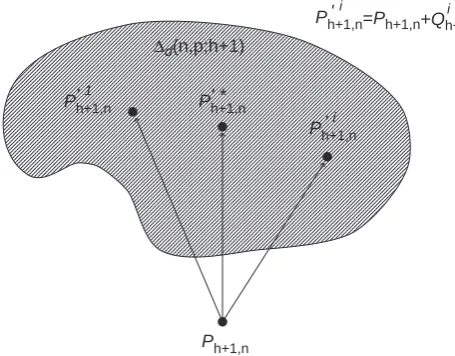
the set of all polynomial setsPh+1,nwith the(n,p)the maxi-mal two degrees andh+1 elements. IfPh+1,n∈Π(n,p;h+1)
we can define an (n,p)-ordered perturbed set
Ph′+1,n=Ph+1,n−Qh+1,n∈Π(n,p;h+1) (20)
={p′i(s) =pi(s)−qi(s): degqi(s)≤degpi(s)} (21)
This process is described by Figure 1.
Lemma 2 [1]: For a set Ph+1,n∈Π(n,p;h+1) and an
ω(s)∈R[s] with degω(s)≤p, there always exists a family
of(n,p)-ordered perturbationsQh+1,nand for every element
of this familyPh′+1,n=Ph+1,n−Qh+1,nhas a GCD divisible
byω(s).
Definition 1: LetPh+1,n∈Π(n,p;h+1)andω(s)∈R[s]be
a given polynomial with degω(s) =r≤p. IfΣω={Qh+1,n
}
is the set of all(n,p)-order perturbations
Ph′+1,n=Ph+1,n−Qh+1,n∈Π(n,p;h+1) (22)
with the property that ω(s) is a common factor of the elements of Ph′+1,n. If Q∗h+1,n is the minimal norm element of the set Σω, then ω(s) is referred as an r-order almost common factor of Ph+1,n, and the norm of Q∗h+1,n, denoted
by∥Q∗∥, as thestrength ofω(s). If ω(s)is the GCD of
Ph∗+1,n=Ph+1,n−Q∗h+1,n (23)
then ω(s) will be called an r-order almost GCD of Ph+1,n
with strength∥Q∗∥. A polynomial ˆω(s)of degreerfor which the strength∥Q∗∥is a global minimum will be called ther
-order optimal almost GCD(OA-GCD) of Ph+1,n.
The above definition suggests that any polynomial ω(s)
may be considered as an “approximate GCD”, as long as degω(s)≤p. Important issues in the definition of approxi-mate (optimal approxiapproxi-mate) GCD are the parameterisation of theΣω set, the definition of an appropriate metric forQh+1,n
and the solution of the optimization problem to defineQ∗h+1,n. The set of all resultants corresponding to Π(n,p;h+1) set, will be denoted byΨ(n,p;h+1).
Remark 4: If Ph+1,n, Qh+1,n, Ph′+1,n∈Π(n,p;h+1) are
sets of polynomials andSP,SQ, ¯S′P denote their generalised
resultants, then these resultants are elements ofΨ(n,p;h+1)
thenS′P=SP−SQ.
Theorem 7: Let Ph+1,n∈Π(n,p;h+1) be a set, SP∈
Ψ(n,p;h+1)be the corresponding generalized resultant and letυ(s)∈R[s], degυ(s) =r≤p,υ(0)̸=0. Any perturbation set Qh+1,n ∈Π(n,p;h+1), i.e. Ph′+1,n =Ph+1,n−Qh+1,n,
which has υ(s) as common divisor, has a generalized re-sultantSQ∈Ψ(n,p;h+1)that is expressed as
SQ=SP−S¯P(r∗)Φˆυ=[ 0r S¯P∗
] ˆ
Φυ (24)
where ˆΦυ is the Toeplitz representation of υ(s)and ¯SP∗ ∈
R(p+hn)×(n+p−r) the (n,p)-expanded resultant of a P∗ ∈
Π(n−r,p−r;h+1). Furthermore, if the parameters of ¯SP∗
are such that ¯SP∗ has full rank, then υ(s) is a GCD of set
Ph′+1,n.
Remark 5:The result provides a parameterisation of all perturbationsQh+1,n∈Π(n,p;h+1)which yield setsPh′+1,n
having a GCD with degree at leastrand divided by the given polynomialυ(s). The free parameters are the coefficients of thePh∗+1,n−r ∈Π(n−r,p−r;h+1) set of polynomials. For a set of parameters, υ(s) is a divisor of Ph′+1,n; for generic sets,υ(s)is a GCD ofPh′+1,n. The evaluation of strength of “approximate GCD” has to relate to the coefficients of the polynomials and the Frobenius norm is an appropriate choice.
Corollary 1:Let Ph+1,n∈Π(n,p;h+1)andυ(s)∈R[s],
almost common divisor ofPh+1,nand its strength is defined
as a solution of the following minimization problem:
f(P,P∗) =min ∀P∗
SP−
[
0r S¯P∗
] ˆ
ΦυF (25)
where P∗∈Π(n,p;h+1). Furthermore υ(s) is an r-order almost GCD of Ph+1,n if the minimal corresponds to a
coprime setP∗ or to full rankSP∗.
The optimization problem defining the strength of any order approximate GCD is now used to investigate the “best” amongst all approximate GCDs of a degree r. We consider polynomialsυ(s),υ(0)̸=0.
Optimisation Problem [1]:This can be expressed as
f1(P,P∗),∥Φˆυ∥F·f(P,P∗) (26)
=min ∀P∗{∥SP−
[
0r S¯P∗
]ˆ
Φυ∥F· ∥Φυ∥F} (27)
=min
∀P∗ ∥SPΦυ−
[
0r S¯P∗
]
∥F (28)
whereP,Φυ have the structure defined byυ(s)of degreer. Theorem 8 [1]: Consider the set of polynomials P∈
Π(n,p;h+1)andSP be its Sylvester matrix. Then,
1) For a certain approximate GCDυ(s)of degree k, the perturbed set ˜Pcorresponding to minimal perturbation applied on P, such that υ(s)becomes an exact GCD, is defined by:
SP˜=S˜
′
PΦˆυ=
[
0k Sˆ2P
]ˆ
Φυ (29)
2) The strength of an arbitrary υ(s) of degree k is
f(P,P∗) =min ∀P∗
S˜′
PΦυF.
3) The optimal approximate GCD of degree
k is a φ(s) defined by solving f(P,P∗) =
min ∀P∗ degφ(s)=k
{S˜′
PΦφF
}
.
The optimization problem defined in the above Theorem is non-convex. Computational algorithms for for calculating the optimal approximate GCD are currently under investigation.
V. GRASSMANN INVARIANTS, APPROXIMATE ZERO POLYNOMIALS AND DISTANCE PROBLEMS
The characterisation of the “approximate GCD” and its “optimal” version provides the means to define the respective approximate zero polynomials for different classes of linear systems properties, which cover the cases: (a) Approximate zero polynomial based on n(s)∧; (b) Approximate input decoupling zero polynomialbased onb(s)∧; (c)Approximate invariant input decoupling polynomial based on r(s)∧; (d)
Approximate output decoupling polynomial based onc(s)∧; (e) Approximate invariant output decoupling polynomial
based onq(s)∧.
Note that such polynomial multi-vectors have to satisfy the corresponding set of QPRs and this makes the computation of the approximate polynomials a more difficult problem. We shall develop the results for the case of a general polynomial matrix.
Corollary 2:LetΠ(n,p;h+1)be the set of all polynomial sets Ph+1,n with h+1 elements and with the two higher
degrees(n,p),n≥p and letSPbe the Sylvester resultant of
the general setPh+1,n. The variety ofPN−1which characterise
all sets Ph+1,n having a GCD with degree d, 0<d ≤p is
defined by the set of equationsCn+p−d+1(SP) =0.
The above defines a variety∆d(n,p;h+1)described by the polynomial equations in the coefficients of the vectorp
h+1,n,
or the point Ph+1,n of PN−1, and will be called thed-GCD
varietyof PN−1. This characterises all sets in Pi(n,p;h+1)
with a GCD of degreed. The definition of the the “optimal GCD” is thus a problem of finding the distance of a given setPh+1,n from the variety∆d(n,p;h+1). For anyPh+1,n∈
Π(n,p;h+1)this distance is defined by
d(P,∆) = min ∀P∗,φ
SP−
[
0k S¯P∗
]ˆ
ΦφF (30)
φ(s)∈R[s],P∗∈Π(n−k,p−k;h+1), degφ(s) =k, the k -distance ofPh+1,nfrom the thek-GCD variety∆k(n,p;h+1)
and ˜φ(s)emerges as a solution to an optimisation problem and it is the k-optimal approximate GCD and the value
d(P,∆) is its k-strenght. For polynomial matrices we can extend the scalar definition of the approximate GCD as follows:
Definition 2: Consider the coprime polynomial matrix
T(s)∈Rq×r[s]and let∆T(s)∈Rq×r[s]be an arbitrary matrix
such that
T(s) +∆T(s) =Tb(s) =Te(s)R(s) (31)
whereR(s)∈Rr×r[s]. ThenR(s) will be called an
approxi-mate matrix divisorof T(s).
The above definition may be interpreted using exterior products as an extension of the problem defined for poly-nomial vector sets. The difference between general sets of vectors and those generated from polynomial matrices by taking exterior products is that the latter must satisfy the decomposability conditions [3] and in turn they define another variety of the Grassmann type.
Consider now the set of polynomial vectorsΠ(n,p;h+1)
and let Π∧(n,p;h+1) be its subset of the decomposable polynomial vectors p(s)∈Rσ[s], which correspond to the
q×rpolynomial matrices with degreen. The setΠ∧(n,p;h+
1) is defined as the Grassmann variety G(q,r;R[s]) of the projective space Pσ−1(R[s]). The way we can extend the scalar results is based on:
(i)Parameterise the perturbations that move a general set
Pσ,n, to a set Pσ′,n=Pσ,n+Qσ,n∈∆k(n,p;σ)where initially
Qσ,nandP′σ,nare free.
(ii) For the scalar results to be transferred back to the polynomial matrices the setsPσ′,nhave to be decomposable multi-vectors which are denoted by Π∧(n,p;σ). The latter set will be referred to as then-order subsetof the Grassmann varietyG(q,r;R[s])and the setsPσ′,n must be such that
Pσ′,n∈Π(n,p;σ)∩∆k(n,p;σ) =∆∧kΠ(n,p;σ) (32)
where ∆∧kΠ(n,p;σ) is the decomposable subset of
∆k(n,p;σ). Parameterising all setsPσ′,n provides the means
the intersection variety defined by the corresponding set of QPRs and the equations of the GCD variety. Some preliminary results on this problem are stated below:
Lemma 3:The following properties hold true:
1) Π∧(n,p;h+1)is proper subset Π(n,p;h+1)ifr̸=1 andq̸=r−1.
2) Π∧(n,p;h+1) =Π(n,p;h+1) if either r=1 orq= r−1.
3) The set ∆∧kΠ(n,p;σ) is always nonempty. The result is a direct implication of the decomposability conditions for multivectors [3].
Theorem 9:LetPσ,n∈Π∧(n,p;σ)and denote byd(P,∆k),
d(P,∆∧k)the distance from∆k(n,p;σ)and∆∧k(n,p;σ)
respec-tively. The following hold true:
1) If q=r−1 or r=1, then the solutions of the two optimisation problems are identical and d(P,∆k) =
d(P,∆∧k).
2) If q̸=r−1 and r̸=1, then d(P,∆k)≤d(P,∆∧k).
Remark 6:For polynomial matrices this distance problem is defined on the set Ph+1,n of Π(n,p;h+1) from the
intersection of the varieties ∆d(n,p;h+1)andG(q,r;R[s]).
The above suggests that the Grassmann distance problem has to be considered only when q̸=r−1 and r̸=1. The Grassmann distance problem requires the study of some additional topics linked to algebraic geometry and exterior algebra such as: (i) Parameterisation of all decomposable sets P with a fixed order n; (ii) Characterisation of the set
∆∧
k(n,p;σ) and its properties. For the special case r=1,
q=r−1 the distance d(P,∆k) is reduced to that of the
polynomial vector case since we guarantee decomposability.
xxxxxxxxxxxxxxxxxxxxxxxxxxxxxxxxxxxxxxxxxxxxxxxxxxxxxxxxxxxxxxxxxxxxxxxxxxxxxxxxxxxxxxxxxxxxxxxxxxxxxxxxxxxxxxxxxx xxxxxxxxxxxxxxxxxxxxxxxxxxxxxxxxxxxxxxxxxxxxxxxxxxxxxxxxxxxxxxxxxxxxxxxxxxxxxxxxxxxxxxxxxxxxxxxxxxxxxxxxxxxxxxxxxx xxxxxxxxxxxxxxxxxxxxxxxxxxxxxxxxxxxxxxxxxxxxxxxxxxxxxxxxxxxxxxxxxxxxxxxxxxxxxxxxxxxxxxxxxxxxxxxxxxxxxxxxxxxxxxxxxx xxxxxxxxxxxxxxxxxxxxxxxxxxxxxxxxxxxxxxxxxxxxxxxxxxxxxxxxxxxxxxxxxxxxxxxxxxxxxxxxxxxxxxxxxxxxxxxxxxxxxxxxxxxxxxxxxx xxxxxxxxxxxxxxxxxxxxxxxxxxxxxxxxxxxxxxxxxxxxxxxxxxxxxxxxxxxxxxxxxxxxxxxxxxxxxxxxxxxxxxxxxxxxxxxxxxxxxxxxxxxxxxxxxx xxxxxxxxxxxxxxxxxxxxxxxxxxxxxxxxxxxxxxxxxxxxxxxxxxxxxxxxxxxxxxxxxxxxxxxxxxxxxxxxxxxxxxxxxxxxxxxxxxxxxxxxxxxxxxxxxx xxxxxxxxxxxxxxxxxxxxxxxxxxxxxxxxxxxxxxxxxxxxxxxxxxxxxxxxxxxxxxxxxxxxxxxxxxxxxxxxxxxxxxxxxxxxxxxxxxxxxxxxxxxxxxxxxx xxxxxxxxxxxxxxxxxxxxxxxxxxxxxxxxxxxxxxxxxxxxxxxxxxxxxxxxxxxxxxxxxxxxxxxxxxxxxxxxxxxxxxxxxxxxxxxxxxxxxxxxxxxxxxxxxx xxxxxxxxxxxxxxxxxxxxxxxxxxxxxxxxxxxxxxxxxxxxxxxxxxxxxxxxxxxxxxxxxxxxxxxxxxxxxxxxxxxxxxxxxxxxxxxxxxxxxxxxxxxxxxxxxx xxxxxxxxxxxxxxxxxxxxxxxxxxxxxxxxxxxxxxxxxxxxxxxxxxxxxxxxxxxxxxxxxxxxxxxxxxxxxxxxxxxxxxxxxxxxxxxxxxxxxxxxxxxxxxxxxx xxxxxxxxxxxxxxxxxxxxxxxxxxxxxxxxxxxxxxxxxxxxxxxxxxxxxxxxxxxxxxxxxxxxxxxxxxxxxxxxxxxxxxxxxxxxxxxxxxxxxxxxxxxxxxxxxx xxxxxxxxxxxxxxxxxxxxxxxxxxxxxxxxxxxxxxxxxxxxxxxxxxxxxxxxxxxxxxxxxxxxxxxxxxxxxxxxxxxxxxxxxxxxxxxxxxxxxxxxxxxxxxxxxx xxxxxxxxxxxxxxxxxxxxxxxxxxxxxxxxxxxxxxxxxxxxxxxxxxxxxxxxxxxxxxxxxxxxxxxxxxxxxxxxxxxxxxxxxxxxxxxxxxxxxxxxxxxxxxxxxx xxxxxxxxxxxxxxxxxxxxxxxxxxxxxxxxxxxxxxxxxxxxxxxxxxxxxxxxxxxxxxxxxxxxxxxxxxxxxxxxxxxxxxxxxxxxxxxxxxxxxxxxxxxxxxxxxx xxxxxxxxxxxxxxxxxxxxxxxxxxxxxxxxxxxxxxxxxxxxxxxxxxxxxxxxxxxxxxxxxxxxxxxxxxxxxxxxxxxxxxxxxxxxxxxxxxxxxxxxxxxxxxxxxx xxxxxxxxxxxxxxxxxxxxxxxxxxxxxxxxxxxxxxxxxxxxxxxxxxxxxxxxxxxxxxxxxxxxxxxxxxxxxxxxxxxxxxxxxxxxxxxxxxxxxxxxxxxxxxxxxx xxxxxxxxxxxxxxxxxxxxxxxxxxxxxxxxxxxxxxxxxxxxxxxxxxxxxxxxxxxxxxxxxxxxxxxxxxxxxxxxxxxxxxxxxxxxxxxxxxxxxxxxxxxxxxxxxx xxxxxxxxxxxxxxxxxxxxxxxxxxxxxxxxxxxxxxxxxxxxxxxxxxxxxxxxxxxxxxxxxxxxxxxxxxxxxxxxxxxxxxxxxxxxxxxxxxxxxxxxxxxxxxxxxx xxxxxxxxxxxxxxxxxxxxxxxxxxxxxxxxxxxxxxxxxxxxxxxxxxxxxxxxxxxxxxxxxxxxxxxxxxxxxxxxxxxxxxxxxxxxxxxxxxxxxxxxxxxxxxxxxx xxxxxxxxxxxxxxxxxxxxxxxxxxxxxxxxxxxxxxxxxxxxxxxxxxxxxxxxxxxxxxxxxxxxxxxxxxxxxxxxxxxxxxxxxxxxxxxxxxxxxxxxxxxxxxxxxx xxxxxxxxxxxxxxxxxxxxxxxxxxxxxxxxxxxxxxxxxxxxxxxxxxxxxxxxxxxxxxxxxxxxxxxxxxxxxxxxxxxxxxxxxxxxxxxxxxxxxxxxxxxxxxxxxx xxxxxxxxxxxxxxxxxxxxxxxxxxxxxxxxxxxxxxxxxxxxxxxxxxxxxxxxxxxxxxxxxxxxxxxxxxxxxxxxxxxxxxxxxxxxxxxxxxxxxxxxxxxxxxxxxx xxxxxxxxxxxxxxxxxxxxxxxxxxxxxxxxxxxxxxxxxxxxxxxxxxxxxxxxxxxxxxxxxxxxxxxxxxxxxxxxxxxxxxxxxxxxxxxxxxxxxxxxxxxxxxxxxx xxxxxxxxxxxxxxxxxxxxxxxxxxxxxxxxxxxxxxxxxxxxxxxxxxxxxxxxxxxxxxxxxxxxxxxxxxxxxxxxxxxxxxxxxxxxxxxxxxxxxxxxxxxxxxxxxx xxxxxxxxxxxxxxxxxxxxxxxxxxxxxxxxxxxxxxxxxxxxxxxxxxxxxxxxxxxxxxxxxxxxxxxxxxxxxxxxxxxxxxxxxxxxxxxxxxxxxxxxxxxxxxxxxx xxxxxxxxxxxxxxxxxxxxxxxxxxxxxxxxxxxxxxxxxxxxxxxxxxxxxxxxxxxxxxxxxxxxxxxxxxxxxxxxxxxxxxxxxxxxxxxxxxxxxxxxxxxxxxxxxx xxxxxxxxxxxxxxxxxxxxxxxxxxxxxxxxxxxxxxxxxxxxxxxxxxxxxxxxxxxxxxxxxxxxxxxxxxxxxxxxxxxxxxxxxxxxxxxxxxxxxxxxxxxxxxxxxx xxxxxxxxxxxxxxxxxxxxxxxxxxxxxxxxxxxxxxxxxxxxxxxxxxxxxxxxxxxxxxxxxxxxxxxxxxxxxxxxxxxxxxxxxxxxxxxxxxxxxxxxxxxxxxxxxx xxxxxxxxxxxxxxxxxxxxxxxxxxxxxxxxxxxxxxxxxxxxxxxxxxxxxxxxxxxxxxxxxxxxxxxxxxxxxxxxxxxxxxxxxxxxxxxxxxxxxxxxxxxxxxxxxx xxxxxxxxxxxxxxxxxxxxxxxxxxxxxxxxxxxxxxxxxxxxxxxxxxxxxxxxxxxxxxxxxxxxxxxxxxxxxxxxxxxxxxxxxxxxxxxxxxxxxxxxxxxxxxxxxx xxxxxxxxxxxxxxxxxxxxxxxxxxxxxxxxxxxxxxxxxxxxxxxxxxxxxxxxxxxxxxxxxxxxxxxxxxxxxxxxxxxxxxxxxxxxxxxxxxxxxxxxxxxxxxxxxx xxxxxxxxxxxxxxxxxxxxxxxxxxxxxxxxxxxxxxxxxxxxxxxxxxxxxxxxxxxxxxxxxxxxxxxxxxxxxxxxxxxxxxxxxxxxxxxxxxxxxxxxxxxxxxxxxx xxxxxxxxxxxxxxxxxxxxxxxxxxxxxxxxxxxxxxxxxxxxxxxxxxxxxxxxxxxxxxxxxxxxxxxxxxxxxxxxxxxxxxxxxxxxxxxxxxxxxxxxxxxxxxxxxx xxxxxxxxxxxxxxxxxxxxxxxxxxxxxxxxxxxxxxxxxxxxxxxxxxxxxxxxxxxxxxxxxxxxxxxxxxxxxxxxxxxxxxxxxxxxxxxxxxxxxxxxxxxxxxxxxx xxxxxxxxxxxxxxxxxxxxxxxxxxxxxxxxxxxxxxxxxxxxxxxxxxxxxxxxxxxxxxxxxxxxxxxxxxxxxxxxxxxxxxxxxxxxxxxxxxxxxxxxxxxxxxxxxx xxxxxxxxxxxxxxxxxxxxxxxxxxxxxxxxxxxxxxxxxxxxxxxxxxxxxxxxxxxxxxxxxxxxxxxxxxxxxxxxxxxxxxxxxxxxxxxxxxxxxxxxxxxxxxxxxx xxxxxxxxxxxxxxxxxxxxxxxxxxxxxxxxxxxxxxxxxxxxxxxxxxxxxxxxxxxxxxxxxxxxxxxxxxxxxxxxxxxxxxxxxxxxxxxxxxxxxxxxxxxxxxxxxx xxxxxxxxxxxxxxxxxxxxxxxxxxxxxxxxxxxxxxxxxxxxxxxxxxxxxxxxxxxxxxxxxxxxxxxxxxxxxxxxxxxxxxxxxxxxxxxxxxxxxxxxxxxxxxxxxx xxxxxxxxxxxxxxxxxxxxxxxxxxxxxxxxxxxxxxxxxxxxxxxxxxxxxxxxxxxxxxxxxxxxxxxxxxxxxxxxxxxxxxxxxxxxxxxxxxxxxxxxxxxxxxxxxx xxxxxxxxxxxxxxxxxxxxxxxxxxxxxxxxxxxxxxxxxxxxxxxxxxxxxxxxxxxxxxxxxxxxxxxxxxxxxxxxxxxxxxxxxxxxxxxxxxxxxxxxxxxxxxxxxx xxxxxxxxxxxxxxxxxxxxxxxxxxxxxxxxxxxxxxxxxxxxxxxxxxxxxxxxxxxxxxxxxxxxxxxxxxxxxxxxxxxxxxxxxxxxxxxxxxxxxxxxxxxxxxxxxx xxxxxxxxxxxxxxxxxxxxxxxxxxxxxxxxxxxxxxxxxxxxxxxxxxxxxxxxxxxxxxxxxxxxxxxxxxxxxxxxxxxxxxxxxxxxxxxxxxxxxxxxxxxxxxxxxx xxxxxxxxxxxxxxxxxxxxxxxxxxxxxxxxxxxxxxxxxxxxxxxxxxxxxxxxxxxxxxxxxxxxxxxxxxxxxxxxxxxxxxxxxxxxxxxxxxxxxxxxxxxxxxxxxx xxxxxxxxxxxxxxxxxxxxxxxxxxxxxxxxxxxxxxxxxxxxxxxxxxxxxxxxxxxxxxxxxxxxxxxxxxxxxxxxxxxxxxxxxxxxxxxxxxxxxxxxxxxxxxxxxx xxxxxxxxxxxxxxxxxxxxxxxxxxxxxxxxxxxxxxxxxxxxxxxxxxxxxxxxxxxxxxxxxxxxxxxxxxxxxxxxxxxxxxxxxxxxxxxxxxxxxxxxxxxxxxxxxx xxxxxxxxxxxxxxxxxxxxxxxxxxxxxxxxxxxxxxxxxxxxxxxxxxxxxxxxxxxxxxxxxxxxxxxxxxxxxxxxxxxxxxxxxxxxxxxxxxxxxxxxxxxxxxxxxx xxxxxxxxxxxxxxxxxxxxxxxxxxxxxxxxxxxxxxxxxxxxxxxxxxxxxxxxxxxxxxxxxxxxxxxxxxxxxxxxxxxxxxxxxxxxxxxxxxxxxxxxxxxxxxxxxx xxxxxxxxxxxxxxxxxxxxxxxxxxxxxxxxxxxxxxxxxxxxxxxxxxxxxxxxxxxxxxxxxxxxxxxxxxxxxxxxxxxxxxxxxxxxxxxxxxxxxxxxxxxxxxxxxx xxxxxxxxxxxxxxxxxxxxxxxxxxxxxxxxxxxxxxxxxxxxxxxxxxxxxxxxxxxxxxxxxxxxxxxxxxxxxxxxxxxxxxxxxxxxxxxxxxxxxxxxxxxxxxxxxx xxxxxxxxxxxxxxxxxxxxxxxxxxxxxxxxxxxxxxxxxxxxxxxxxxxxxxxxxxxxxxxxxxxxxxxxxxxxxxxxxxxxxxxxxxxxxxxxxxxxxxxxxxxxxxxxxx xxxxxxxxxxxxxxxxxxxxxxxxxxxxxxxxxxxxxxxxxxxxxxxxxxxxxxxxxxxxxxxxxxxxxxxxxxxxxxxxxxxxxxxxxxxxxxxxxxxxxxxxxxxxxxxxxx xxxxxxxxxxxxxxxxxxxxxxxxxxxxxxxxxxxxxxxxxxxxxxxxxxxxxxxxxxxxxxxxxxxxxxxxxxxxxxxxxxxxxxxxxxxxxxxxxxxxxxxxxxxxxxxxxx xxxxxxxxxxxxxxxxxxxxxxxxxxxxxxxxxxxxxxxxxxxxxxxxxxxxxxxxxxxxxxxxxxxxxxxxxxxxxxxxxxxxxxxxxxxxxxxxxxxxxxxxxxxxxxxxxx xxxxxxxxxxxxxxxxxxxxxxxxxxxxxxxxxxxxxxxxxxxxxxxxxxxxxxxxxxxxxxxxxxxxxxxxxxxxxxxxxxxxxxxxxxxxxxxxxxxxxxxxxxxxxxxxxx xxxxxxxxxxxxxxxxxxxxxxxxxxxxxxxxxxxxxxxxxxxxxxxxxxxxxxxxxxxxxxxxxxxxxxxxxxxxxxxxxxxxxxxxxxxxxxxxxxxxxxxxxxxxxxxxxx xxxxxxxxxxxxxxxxxxxxxxxxxxxxxxxxxxxxxxxxxxxxxxxxxxxxxxxxxxxxxxxxxxxxxxxxxxxxxxxxxxxxxxxxxxxxxxxxxxxxxxxxxxxxxxxxxx xxxxxxxxxxxxxxxxxxxxxxxxxxxxxxxxxxxxxxxxxxxxxxxxxxxxxxxxxxxxxxxxxxxxxxxxxxxxxxxxxxxxxxxxxxxxxxxxxxxxxxxxxxxxxxxxxx xxxxxxxxxxxxxxxxxxxxxxxxxxxxxxxxxxxxxxxxxxxxxxxxxxxxxxxxxxxxxxxxxxxxxxxxxxxxxxxxxxxxxxxxxxxxxxxxxxxxxxxxxxxxxxxxxx xxxxxxxxxxxxxxxxxxxxxxxxxxxxxxxxxxxxxxxxxxxxxxxxxxxxxxxxxxxxxxxxxxxxxxxxxxxxxxxxxxxxxxxxxxxxxxxxxxxxxxxxxxxxxxxxxx xxxxxxxxxxxxxxxxxxxxxxxxxxxxxxxxxxxxxxxxxxxxxxxxxxxxxxxxxxxxxxxxxxxxxxxxxxxxxxxxxxxxxxxxxxxxxxxxxxxxxxxxxxxxxxxxxx xxxxxxxxxxxxxxxxxxxxxxxxxxxxxxxxxxxxxxxxxxxxxxxxxxxxxxxxxxxxxxxxxxxxxxxxxxxxxxxxxxxxxxxxxxxxxxxxxxxxxxxxxxxxxxxxxx xxxxxxxxxxxxxxxxxxxxxxxxxxxxxxxxxxxxxxxxxxxxxxxxxxxxxxxxxxxxxxxxxxxxxxxxxxxxxxxxxxxxxxxxxxxxxxxxxxxxxxxxxxxxxxxxxx xxxxxxxxxxxxxxxxxxxxxxxxxxxxxxxxxxxxxxxxxxxxxxxxxxxxxxxxxxxxxxxxxxxxxxxxxxxxxxxxxxxxxxxxxxxxxxxxxxxxxxxxxxxxxxxxxx xxxxxxxxxxxxxxxxxxxxxxxxxxxxxxxxxxxxxxxxxxxxxxxxxxxxxxxxxxxxxxxxxxxxxxxxxxxxxxxxxxxxxxxxxxxxxxxxxxxxxxxxxxxxxxxxxx xxxxxxxxxxxxxxxxxxxxxxxxxxxxxxxxxxxxxxxxxxxxxxxxxxxxxxxxxxxxxxxxxxxxxxxxxxxxxxxxxxxxxxxxxxxxxxxxxxxxxxxxxxxxxxxxxx xxxxxxxxxxxxxxxxxxxxxxxxxxxxxxxxxxxxxxxxxxxxxxxxxxxxxxxxxxxxxxxxxxxxxxxxxxxxxxxxxxxxxxxxxxxxxxxxxxxxxxxxxxxxxxxxxx xxxxxxxxxxxxxxxxxxxxxxxxxxxxxxxxxxxxxxxxxxxxxxxxxxxxxxxxxxxxxxxxxxxxxxxxxxxxxxxxxxxxxxxxxxxxxxxxxxxxxxxxxxxxxxxxxx xxxxxxxxxxxxxxxxxxxxxxxxxxxxxxxxxxxxxxxxxxxxxxxxxxxxxxxxxxxxxxxxxxxxxxxxxxxxxxxxxxxxxxxxxxxxxxxxxxxxxxxxxxxxxxxxxx xxxxxxxxxxxxxxxxxxxxxxxxxxxxxxxxxxxxxxxxxxxxxxxxxxxxxxxxxxxxxxxxxxxxxxxxxxxxxxxxxxxxxxxxxxxxxxxxxxxxxxxxxxxxxxxxxx
∆d(n,p;h+1)
Ph+1,n
Ph+1,n Ph+1,n' 1
Ph+1,n=Ph+1,n+Qh+1,n
' *
Ph+1,n' i
[image:7.595.60.288.456.634.2]'i i
Fig. 1. The notion of “approximate GCD”
VI. CONCLUSIONS
The paper uses the recently introduced notion of “approx-imate GCD” of a set of polynomials [1] and the charac-terization of controllability and observability properties in
terms of exterior products and associated Pl¨ucker matrices of controllability and observability pencils [9] to define distance from the set of uncontrollable, unobservable systems, as well as the corresponding approximate decoupling polynomials; furthermore, the use of the restriction pencilsR(s)andQ(s)
allows the definition of the distance of the state feedback, output injection orbits from uncontrollable, unobservable families respectively. The main distinctive feature of the approach, is the definition of distance of the orbits of systems from the uncontrollable, unobservable sets, as well as the definition of the approximate decoupling polynomials. The paper also extends the notion of approximate GCD of a set of polynomials to the case of approximate matrix divisors. It has been shown that this problem is equivalent to a distance problem from the intersection of two varieties and it is much harder than the polynomial vectors case. Our approach is based on the optimal approximate GCD and when this is applied to linear systems introduces new system invariants with significance in defining system properties under parameter variations on the corresponding model. The optimization problem is non-convex and developing methodology for computing this distance is a problem of current research.
REFERENCES
[1] N. Karcanias, S. Fatouros, M. Mitrouli and G. Halikias, Approximate greatest common divisor of many polynomials, generalised resultants,
and strength of approximation,Comput & Maths with Applications,
vol. 51(12), 2006, pp 1817-1830.
[2] N. Karcanias, C. Giannakopoulos and M. Hubbard, Almost zeros of
a set of polynomials of R[s], Int. J. Control, vol. 38(6), 1983, pp
1213-1238.
[3] M. Marcus, Finite dimensional multilinear algebra (in two parts),
Marcel Deker, New York, 1973.
[4] N. Karcanias and C. Giannakopoulos, On Grassmann invariants and almost zeros of linear systems and the determinantal zero, pole
assignment problem,Int. J. Control, vol 40, 1984.
[5] N. Karcanias and C. Giannakopoulos, Necessary and Sufficient
Con-ditions for Zero Assignment by Constant Squaring Down, Linear
Algebra and Its Applications, Special Issue on Control Theory, vol. 122/123/124, pp 415-446, 1989.
[6] H.H. Rosenbrock, State Space and Multivariable Theory, Nelson,
London, 1970.
[7] T. Kailath,Linear Systems, Prentice Hall, Englewood Cliffs, NJ, 1980.
[8] G.D. Forney, Minimal Bases of Rational Vector Spaces with
Applica-tions to Multivariable Systems,SIAM J. Control, vol. 13, pp 493-520,
1975.
[9] N. Karcanias and J. Leventides, Grassman Invariants, Matrix Pencils and Linear System Properties,Linear Algebra & Its Applications, vol. 241-243, pp 705-731, 1996.
[10] J. Leventides and N. Karcanias N, Structured Squaring Down and Zero
Assignment,Int. J. Control, vol. 81, pp 294-306, 2008.
[11] S. Barnett, Matrices Methods and Applications, Clarendon Press,
Oxford, 1990.
[12] S. Fatouros and N. Karcanias, Resultant Properties of GCD of polynom
and a Factorisation Represent of GCD,Int. J. of Control, vol. 76, pp
1666-1683, 2003.
[13] S. Jaffe and N. Karcanias, Matrix pencil characterisation of almost
(A,B)-invariant subspaces: A classification of geometric concepts,Int. J. Control, vol. 33, pp 51-93, 1981.
[14] N. Karcanias and P. Macbean, Structural invariants and canonical
forms of linear multivariable systems, 3rd IMA Intern Conf. On
Control Theory, Academic Press, pp 257-282, 1981.
[15] D.L. Boley and W.S. Lu, Measuring how far a controllable system is
from an uncontrollable one,IEEE Tran. Auto. Contr., vol AC-31(3),