Modelling and simulation of advanced non-linear autopilot designs

Modeling and Simulation of Advanced Non-Linear Autopilot Designs

Joseph Brindley and John M Counsell University of Strathclyde

16 Richmond Street Glasgow, G1 1XQ, Scotland, UK.

[email protected] [email protected]

Keywords: Non-linear, Discontinuous, Control Systems, ESL

Abstract

This paper presents the simulation in ESL of a non-linear 6 degree-of-freedom missile model with an advanced, non-linear, multivariable autopilot designed using Rate Actuated Inverse Dynamics (RAID) methods. High performance control of non-linear systems requires the design of advanced, non-linear control systems, such as those used in autopilot design. Traditional linear control system design and analysis techniques are not sufficient for non-linear systems and current non-linear analysis methods are extremely limited. Therefore, the only method available to fully assess the performance of non-linear controller designs is simulation of the non-linear system. For this reason it is an essential part of the analysis and design process of these types of controllers. Non-linear dynamics can be continuous or discontinuous, the aerodynamics of a missile are non-linear but since they are continuous they do not represent a simulation challenge. However, there are multiple sets of discontinuous dynamics present in both the missile control surface model and the autopilot which can lead to multiple discontinuities being reached simultaneously, providing a challenging modeling exercise. The paper demonstrates how this kind of behavior can be successfully modeled and simulated within ESL using a simple switching logic.

1. NOMENCLATURE

d = missile diameter e = error signal

Ixx = moment of inertia about x axis Iyy = moment of inertia about y axis Izz = moment of inertia about z axis KI = integral gain matrix

KP = proportional gain matrix φ = missile angle of incidence λ = missile aerodynamic roll angle m = missile mass

M = Mach number

John G Pearce

ISIM International Simulation Limited 161 Claremont Road

Salford, M6 8PA, UK [email protected]

Pd = dynamic pressure p = roll rate

q = pitchrate r = yaw rate

η = control surface deflection eta ζ = control surface deflection zeta ξ = control surface deflection xi S = wetted surface area

Ta = air temperature uc = control signal

= estimated equivalent control signal Vm = total forward velocity

v = missile forward velocity w = missile vertical velocity y = system output

2. INTRODUCTION

The development of advanced non-linear controller designs has led to simulation becoming a key stage in the analysis and design of control systems. This is because classical linear design and analysis techniques, such as route locus and bode plots [1], are no longer fully applicable if the system in question is non-linear. Linear analysis methods have been adapted to analyze non-linear systems, for instance the describing function method [2], but their use is very limited. Methods that are able to determine stability if the system is non-linear are available (such as the Lyapunov stability criterion [1]), however, again these techniques are extremely limited and even more so if the system is both non-linear and discontinuous. Even if the controller being designed is fully linear, in reality, the system that you are trying to control will almost always be non-linear and so in order to properly assess the performance of the control system a full non-linear simulation is required.

aircraft are non-linear, but since these can generally be considered continuous they do not pose the greatest design challenge. The most significant non-linear behavior is due to the actuator driving the control surfaces having deflection and rate of deflection limits. This discontinuous feature of the actuator often results in linear autopilots being designed so that the limits are never reached [3]. However, high performance non-linear controller designs such as Robust Inverse Dynamics Estimation (RIDE) [4] and Rate Actuated Inverse Dynamics (RAID) [5] purposefully push the system to its performance limits. Therefore, the importance of simulation when designing these controllers is doubled as both the aircraft and the autopilot is non-linear. This places extra emphasis on the accuracy of simulation when, as there are multiple actuators, multiple limits are being reached simultaneously. It is the challenge of accurate simulation of discontinuous behavior that is the main focus of this paper.

This paper describes the modeling and simulation using the ESL simulation language of a multivariable missile autopilot designed using RAID methods. Particular attention is paid to the modeling of the actuator limits and the related non-linear conditioning of the autopilot. Discontinuity detection in ESL is discussed and finally simulation results are presented.

3. DISCONTINUITY TREATMENT IN ESL

All the modeling and simulation presented in this paper was done so using the ESL simulation language and solver. ESL is a high level, structured language and can be used for modeling a wide variety of system types described by partial or ordinary differential equations. The solver is advanced in its treatment of discontinuities which makes it particularly well suited to modeling the multiple discontinuities present in the missile dynamics and autopilot algorithm.

Integration algorithms cannot integrate satisfactorily in the presence of discontinuities. A discontinuity is an event which causes the algebraic or differential equations representing the system to suffer a jump or step change in one or more modeling variables. Such events are very common in real systems, that is, limits, dead-space etc.

In mathematical terms the function is piece-wise continuous with a discontinuity representing an abrupt change in a state variable, or its first or higher derivative. A discontinuity within an integration-step invalidates the Taylor series representation of the step, and consequently any of the integration algorithms used.

ESL incorporates an integration-discontinuity control mechanism which accurately and efficiently detects and locates discontinuities. ESL does not allow a discontinuity to occur within an integration-step. It arranges for it to occur after the end of one step and before the beginning of the next, that is, between steps. This would normally lead to a gross time error, however at the end of each step a check is made to see if a discontinuity should have occurred in the

step. If this was the case the last step may be repeated with a shorter step-length based on an interpolation of the discontinuity function (the relational expression describing the discontinuity). The interpolation process is repeated until the step-end occurs just after the point of discontinuity, that is, within specified error bounds. The change to a modeling parameter may then be made, between steps, before proceeding with the simulation of the new state of the system.

As the control mechanism does not allow any change to take effect during an integration-step, the integration routines are protected from the effects of a discontinuity occurring in mid-step.

A feature of ESL’s discontinuity detection mechanism that is particularly relevant to the simulation described in this paper is that it can handle the case where multiple discontinuities occur within one integration step. Once one discontinuity has been detected and its associated action taken, a check is made to see if this has triggered any consequential discontinuities. The process is repeated until all discontinuities occurring within an integration step have been processed in the correct sequence.

In terms of program code, discontinuities are described using two statement structures: the IF clause – which is essentially a switch allowing alternative values to be assigned to a variable, dependent upon the state of a logical expression; and the WHEN statement – which allows actions to be taken at the precise time a logical expressions becomes true. It is found that any discontinuous operation can be represented using a combination of these two statements. Examples of both structures will be found in the code excerpts presented in this paper.

4. OVERVIEW OF THE AUTOPILOT/MISSILE

SYSTEM

Z axes respectively. Therefore, the objective of the control system presented in this paper is the accurate and stable tracking of requested pitch, roll and yaw rates.

Figure 1. Missile body axis

Figure 2. The guided missile system

5. MODELING THE MISSILE SYSTEM

5.1. Aerodynamics

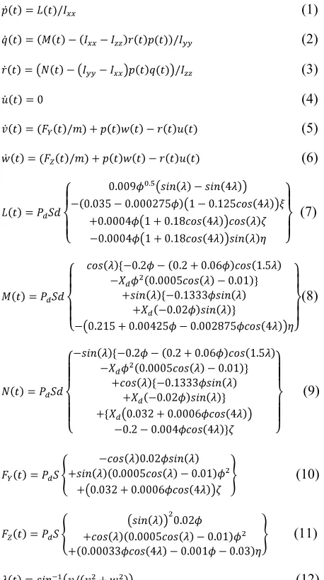
The aerodynamics of the missile are described by a set of non-linear, continuous, differential equations (equations 1-16). A number of assumptions were made in the development of the model[6]:

The aerodynamics are invariant with Mach number and hence the model is only valid for small changes in either altitude or missile velocity. The flexible body dynamics of the missile are not modeled and as such the missile is assumed to be completely rigid.

There are no fin stalling effects. Gravitational effects are ignored

The missile is assumed to have a constant mass, i.e. the effects of fuel being consumed are neglected.

(1)

(2)

(3)

(4)

(5)

(6)

(7)

(8)

(9)

(10)

(11)

(12)

Navigation System

LATAX Controller

Body Rate Controller

Missile

Target position information

Lateral accelerations

Angular velocities (p q r)

Control surface deflections

A

cc

ele

rati

o

n

fe

ed

b

ac

k

Bo

d

y rate

fee

d

b

ac

k

r

w

v p

q X

Y

Z

(13)

(14)

(15)

(16)

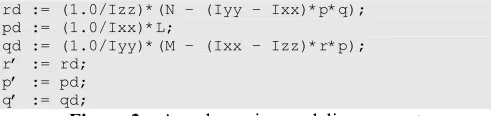
Since the equations are continuous it is a relatively straightforward task to code them in ESL. Figure 3 shows an excerpt of the modeling code.

rd := (1.0/Izz)*(N – (Iyy – Ixx)*p*q); pd := (1.0/Ixx)*L;

qd := (1.0/Iyy)*(M – (Ixx – Izz)*r*p); r’ := rd;

p’ := pd; q’ := qd;

Figure 3. Aerodynamics modeling excerpt

5.2. Control Surface Actuation

The missile being simulated has a cruciform control surface arrangement which is situated at the tail. These control surfaces can be represented as three equivalent deflections; elevator (η), rudder (ζ) and aileron (ξ). The control surfaces of most modern missiles are actuated by high performance D.C. electric motors. The motor can either be modeled in fine detail by explicitly simulating the electronics or a simpler model can be used which captures the important performance characteristics of the motor [6]. In this simulation the later approach was used.

The actuator model can be split into two components; a linear part which approximates the continuous dynamics and a non-linear part which approximates the discontinuous characteristics of the motor (such as deflection limits). Equation 17 describes the linear, continuous dynamics, which are second order. The speed of the linear response is determined by the time constant (τ).

(17)

The non-linear component of the actuator model is both challenging from a modeling and simulation point of view as well being extremely important for the controller design as it places limits on the maximum performance of the missile. The motor which is modeled has two discontinuous limits, a deflection limit and a rate of deflection limit, these are described in Table 1. The deflection limit occurs due to the space considerations of the control surface arrangement as well as the fact that airflow separation will occur once a high enough angle of deflection is reached. Rate of deflection limits of electric motors are generally determined

by the available torque or power of the motor. Since there are three control surface deflections (eta, zeta and xi), there are in total six limits which are to be modeled. An excerpt of the ESL code used to model the limits for eta is shown in Figure 4 (the code is simply repeated for zeta and xi). The first modeling challenge is to ensure that whenever the deflection or rate of deflection limit is reached that the acceleration of the control surface is zero. This problem is overcome through the use of an IF statement which resets the acceleration of the control surface to zero when either of these conditions is met. By doing this the rate limits are also indirectly defined. The second modeling challenge is to ensure that the control surface velocity is zero when the deflection limit is reached. This is achieved by using a WHEN statement which will reset the velocity when the deflection limit is met.

Table 1. Control surface properties

rate_error_eta := ceta_rate - eta_rate;

accl_eta := if (eta>=UL and rate_error_eta>0.0) or (eta<=LL and rate_error_eta<0.0)

or (eta_rate>=UVL and rate_error_eta>0.0) or (eta_rate<=LVL and rate_error_eta<0.0) then 0.0

else rate_error_eta/tau;

eta_rate' := accl_eta;

eta' := eta_rate;

when eta >=UL or eta <=LL then eta_rate := 0.0;

end_when;

Figure 4. Control surface limitations

5.3. Autopilot

The objective of the autopilot in this simulation is the control of the missile body rates, p (roll rate), q (pitch rate) and r (yaw rate). The autopilot was designed using the advanced non-linear controller design method of Rate Actuated Inverse Dynamics (RAID). The RAID controller requests a rate of deflection from each of the control surfaces in order to achieve the requested body rates. A block diagram of the RAID autopilot is shown in Figure 6.

The autopilot is required to fly the missile to its absolute performance limits; a result of this is that the control surfaces will become limited. Thus, the control system must be able to perform safely when these discontinuous non-linearities occur. Safe operation when the

τ = 0.0015 seconds

control surfaces limit in deflection and rate of deflection can be achieved with the RAID design by conditioning the error vector, e. If any one of the control surfaces limit in rate then the entire error vector is reset to zero. If any one of the control surfaces reaches its upper deflection limit and the rate of deflection is equal or greater than zero then the error vector is reset to zero. Similarly if one of the control surfaces reaches its lower deflection limit and the rate of deflection is equal or less than zero then the error vector is reset to zero. This results in a total of twelve reset conditions for the three control surfaces, which may be triggered simultaneously, providing a stern test for the robustness of the integration algorithm. The ESL modeling of the regulator conditioning is accomplished using multiple IF statements, which are shown in Figure 5.

error := if abs(urate1) >= 17.5 then reset else_if abs(urate2) >= 17.5 then reset else_if abs(urate3) >= 17.5 then reset

else_if uvector(1) >= 0.35 and urate1 >= 0.0 then reset

else_if uvector(1) <= -0.35 and urate1 <= 0.0 then reset

else_if uvector(2) >= 0.35 and urate2 >= 0.0 then reset

else_if uvector(2) <= -0.35 and urate2 <= 0.0 then reset

else_if uvector(3) >= 0.35 and urate3 >= 0.0 then reset

else_if uvector(3) <= -0.35 and urate3 <= 0.0 then reset

else yd-w;

Figure 5. Autopilot conditioning

Figure 6. Block diagram of the RAID autopilot

6. SIMULATION RESULTS

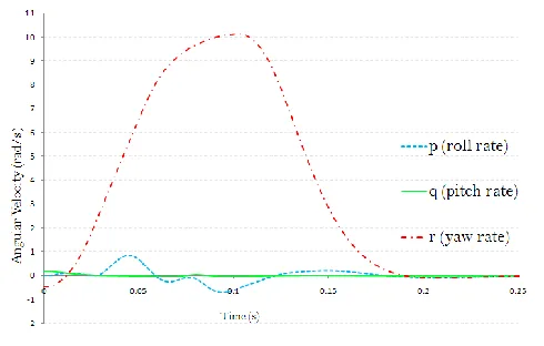
The simulation of the guided missile was performed with the ESL integration step set to 0.0005 seconds. This was chosen as the fasted dynamics present in the system are those of the actuator, which has a time constant of 0.0015. The autopilot was required to track a large yaw rate (r) pulse of 10 radians per second for 0.1 seconds so that the control system would saturate the deflection and rate of deflection of the control surfaces. Figure 7 shows that the autopilot is

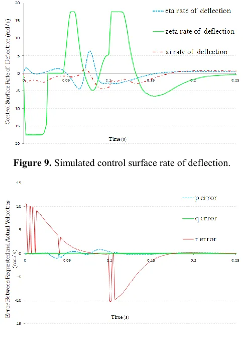
performing extremely well given the non-linear nature of the system. More interesting from a simulation point of view are Figures 8, 9 and 10 which show the saturation of the actuator in deflection and rate of deflection as well as the conditioning of the error signal. Figure 8 shows the control surface zeta reaching its deflection limit from approximately 0.025 to 0.05 seconds. This is preceded by the control surface limiting in rate, so almost the entire time between 0 and 0.05 seconds the actuator is in a non-linear mode of operation. In order for the control system to remain stable during this period the error signal is conditioned resulting in a rapid switching of the vector. This switching occurs again when the actuator becomes limited in rate from approximately 0.1 to 0.125 seconds.

Figure 7. Simulated body rate response

Figure 9. Simulated control surface rate of deflection.

Figure 10. Conditioning of the error vector

7. CONCLUSIONS

A non-linear, discontinuous, multivariable model of a high performance missile has been presented. The modelling of the system in ESL has been described with particular attention paid to the discontinuous features. In order to control the missile an advanced non-linear autopilot is also presented and the modelling in ESL described. It has been demonstrated that complex discontinuous behaviour can be simply modelled with logical statements, which, cause the ESL integration algorithm to be modified when the discontinuities occur. The results of the guided missile simulation are presented which illustrates the discontinuous behaviour of the system described in the paper. The control system presented in this paper could not have been fully designed and analysed without the use of non-linear simulation, this emphasises the dependence of modern, high performance controller design on accurate simulation.

References

[1] Franklin, G., Powell, J. D., Emami-Naeini, A., Feedback

Control of Dynamic Systems, 5th _{ed., Prentice Hall, 2005.}

[2] Fielding, C., Flux, P. K., “Non-linearities in Flight Control

Systems,” Royal Aeronautical Society Journal, Vol. 107, No.

1077, 2003, pp. 673, 686.

[3] Fielding, C., Varga, A., Bennani, S., Selier, M., Advanced

Techniques for Clearance of Flight Control Laws, Springer-Verlag, New York, 2002.

[4] Muir, E., Bradshaw, A., “Control Law Design for a Thrust Vectoring Fighter Aircraft using Robust Inverse Dynamics

Estimation,” Proceedings of the IMechE, Vol. 210, May 1996, pp.

333, 343.

[5] Brindley, J., Counsell, J.M., Zaher, O.S., “Design of a Non-linear Missile Autopilot using Rate Actuated Inverse Dynamics”,

AIAA Guidence, Navigation and Control Conference, Toronto, 2-5 August 2010.