Multi-agent collaborative search : an agent-based memetic multi-objective optimization algorithm applied to space trajectory design

http://pig.sagepub.com/

Engineering

Engineers, Part G: Journal of Aerospace

http://pig.sagepub.com/content/225/11/1211

The online version of this article can be found at:

DOI: 10.1177/0954410011410274

originally published online 5 September 2011

2011 225: 1211

Proceedings of the Institution of Mechanical Engineers, Part G: Journal of Aerospace Engineering

M Vasile and F Zuiani

applied to space trajectory design

Multi-agent collaborative search: an agent-based memetic multi-objective optimization algorithm

Published by:

http://www.sagepublications.com

On behalf of:

Institution of Mechanical Engineers

can be found at:

Proceedings of the Institution of Mechanical Engineers, Part G: Journal of Aerospace Engineering

Additional services and information for

http://pig.sagepub.com/cgi/alerts

Email Alerts:

http://pig.sagepub.com/subscriptions

Subscriptions:

http://www.sagepub.com/journalsReprints.nav

Reprints:

http://www.sagepub.com/journalsPermissions.nav

Permissions:

http://pig.sagepub.com/content/225/11/1211.refs.html

Citations:

What is This?

- Sep 5, 2011

OnlineFirst Version of Record

- Nov 16, 2011

Version of Record

Multi-agent collaborative search: an agent-based

memetic multi-objective optimization algorithm

applied to space trajectory design

M Vasile* andF Zuiani

Department of Mechanical and Aerospace Engineering, University of Strathclyde, Glasgow, UK

The manuscript was received on 2 November 2010 and was accepted after revision for publication on 21 April 2011.

DOI: 10.1177/0954410011410274

Abstract: This article presents an algorithm for multi-objective optimization that blends together a number of heuristics. A population of agents combines heuristics that aim at exploring the search space both globally and in a neighbourhood of each agent. These heuristics are com-plemented with a combination of a local and global archive. The novel agent-based algorithm is tested at first on a set of standard problems and then on three specific problems in space trajec-tory design. Its performance is compared against a number of state-of-the-art multi-objective optimization algorithms that use the Pareto dominance as selection criterion: non-dominated sorting genetic algorithm (NSGA-II), Pareto archived evolution strategy (PAES), multiple objec-tive particle swarm optimization (MOPSO), and multiple trajectory search (MTS). The results demonstrate that the agent-based search can identify parts of the Pareto set that the other algo-rithms were not able to capture. Furthermore, convergence is statistically better although the variance of the results is in some cases higher.

Keywords: multi-objective optimization, trajectory optimization, memetic algorithms, multiagent systems

1 INTRODUCTION

The design of a space mission steps through different phases of increasing complexity. In the first phase, a trade-off analysis of several options is required. The trade-off analysis compares and contrasts design solutions according to different criteria and aims at selecting one or two options that satisfy mission requirements. In mathematical terms, the problem can be formulated as a multi-objective optimization problem.

As part of the trade-off analysis, multiple transfer trajectories to the destination need to be designed. Each transfer should be optimal with respect to a number of criteria. The solution of the associated multi-objective optimization problem, has been

addressed, by many authors, with evolutionary tech-niques. Coverstone-Carollet al. [1] proposed the use of multi-objective genetic algorithms for the optimal design of low-thrust trajectories. Dachwaldet al. [2] proposed the combination of a neurocontroller and of a multi-objective evolutionary algorithm for the design of low-thrust trajectories. In 2005, a study by Leeet al. [3] proposed the use of a Lyapunov control-ler with a multi-objective evolutionary algorithm for the design of low-thrust spirals. More recently, Schu¨ tze et al. [4] proposed some innovative tech-niques to solve multi-objective optimization prob-lems for multi-gravity low-thrust trajectories. Two of the interesting aspects of the work of Schu¨ tze et al. [4] are the archiving ofe- and-approximated solutions, to the known best Pareto front, and the deterministic pre-pruning of the search space [5]. In 2009, Dellnitz et al. [6] proposed the use of multi-objective subdivision techniques for the design of low-thrust transfers to the halo orbits around theL2

libration point in the Earth–Moon system. Minisci

*Corresponding author: Department of Mechanical and Aerospace Engineering, University of Strathclyde, James Weir Building, 75 Montrose Street, Glasgow G1 1XJ, UK.

et al. [7] presented an interesting comparison between an EDA-based algorithm, called MOPED,

and non-dominated sorting genetic algorithm

(NSGA-II) on some constrained and unconstrained multi-impulse orbital transfer problems.

In this article, a hybrid population-based approach that blends a number of heuristics is proposed. In particular, the search for Pareto optimal solutions is carried out globally by a population of agents imple-menting classical social heuristics and more locally by a subpopulation implementing a number of indi-vidualistic actions. The reconstruction of the set of Pareto optimal solutions is handled through two archives: a local and a global one.

The individualistic actions presented in this article are devised to allow each agent to independently con-verge to the Pareto optimal set, thus creating its own partial representation of the Pareto front. Therefore, they can be regarded as memetic mechanisms asso-ciated to a single individual. It will be shown that individualistic actions significantly improve the per-formance of the algorithm.

The algorithm proposed in this article is an exten-sion of the multi-agent collaborative search (MACS), initially proposed in references [8,9], to the solution of multi-objective optimization problems. Such an extension required the modification of the selection criterion, for both global and local moves, to handle Pareto dominance and the inclusion of new heuristics to allow the agents to move toward and along the Pareto front. As part of these new heuristics, this arti-cle introduces a dual archiving mechanism for the management of locally and globally Pareto optimal solutions and an attraction mechanism that improves the convergence of the population.

The new algorithm is here applied to a set of known standard test cases and to three space mission design problems. The space mission design cases in this arti-cle consider spacecraft equipped with a chemical engine and performing a multi-impulse transfer. Although these cases are different from some of the above-mentioned examples, that consider a low-thrust propulsion system, nonetheless the size and complexity of the search space is comparable. Furthermore, it provides a first test benchmark for multi-impulsive problems that have been extensively studied in the single objective case but for which only few comparative studies exist in the multi-objective case [7].

This article is organized as follows: section 2 contains the general formulation of the problem. Section 3 starts with a general introduction to the multi-agent collaborative search algorithm and heu-ristics before going into some of the implementation details. Section 4 contains a set of comparative tests

that demonstrates the effectiveness of the heuristics implemented in MACS. The section briefly introduces the algorithms against which MACS is compared and the two test benchmarks that are used in the numer-ical experiments. It then defines the performance metrics and ends with the results of the comparison.

2 PROBLEM FORMULATION

A general problem in multi-objective optimization is to find the feasible set of solutions that satisfies the following problem

min

x2D fðxÞ ð1Þ

where D is a hyperrectangle defined as D¼

xj jxj 2 ½bjlbuj R, j¼1,. . .,n

and f the vector function

f:D !Rm_{, fðxÞ ¼ ½f1ðxÞ,f2ðxÞ,. . .,fmðxÞ}T

ð2Þ

The optimality of a particular solution is defined through the concept of dominance: with reference to problem (1), a vector y2D is dominated by a vectorx2Diffj(x)<fj(y) for allj¼1,. . .,m. The

rela-tionxaystates thatxdominatesy.

Starting from the concept of dominance, it is pos-sible to associate, to each solution in a set, the scalar dominance index

IdðxjÞ ¼ jfiji^j2Np^xi xjgj ð3Þ

where the symbolW.Wis used to denote the cardinality of a set andNpis the set of the indices of all the

solu-tions. All non-dominated and feasible solutions form the set

X ¼ fx2D jIdðxÞ ¼0g ð4Þ

Therefore, the solution of problem (1) translates into finding the elements ofX. IfXis made of a collection of compact sets of finite measure inRn_{, then once an}

element ofXis identified, it makes sense to explore its neighbourhood to look for other elements of X. On the other hand, the set of non-dominated solu-tions can be disconnected and its elements can form islands inD. Hence, restarting the search process in unexplored regions ofDcan increase the collection of elements ofX.

The setX is the Pareto set and the corresponding image in criteria space is the Pareto front. It is clear that inD, there can be more than oneXlcontaining

solutions that are locally non-dominated, or locally Pareto optimal. The interest is, however, to find the setXgthat contains globally non-dominated, or

3 MULTIAGENT COLLABORATIVE SEARCH

The key motivation behind the development of multi-agent collaborative search was to combine local and global search in a coordinated way such that local convergence is improved while retaining global exploration [9]. This combination of local and global search is achieved by endowing a set of agents with a repertoire of actions producing either the sampling of the whole search space or the explo-ration of a neighbourhood of each agent. More pre-cisely, in the following, global exploration moves will be called collaborative actions while local moves will be called individualistic actions. Note that not all the individualistic actions, described in this article, aim at exploring a neighbourhood of each agent, though. The algorithm presented in this article is a modifi-cation of MACS to tackle multi-objective optimiza-tion problems. In this secoptimiza-tion, the key heuristics underneath MACS will be described together with their modification to handle problem (1) and recon-structX.

3.1 General algorithm description

A populationP0 ofnpopvirtual agents, one for each

solution vectorxi, with i¼1,. . .,npop, is deployed in

D. The population evolves through a number of gen-erations. At every generationk, the dominance index (3) of each agentxi,kin the populationPkis evaluated.

The agents with dominance indexId¼0 form a setXk

of non-dominated solutions. Hence, problem (1) translates into finding a series of sets Xk such that

Xk!Xg for k!kmax with kmax possibly a finite

number.

The position of each agent inDis updated through a number of heuristics. Some are calledcollaborative actions, because they are derived from the interaction of at least two agents and involve the entire popula-tion at one time. The general collaborative heuristic can be expressed in the following form

xk¼xkþSðxkþukÞuk ð5Þ

whereukdepends on the other agents in the

popula-tion andSis a selection function which yields 0 if the candidate point xkþuk is not selected or 1 if it is

selected (section 3.2). In this implementation, a can-didate point is selected if its dominance index is better or equal than the one ofxk. A first restart

mech-anism is then implemented to avoid crowding. This restart mechanism is taken from reference [9] and prevents the agents from overlapping or getting too close. It is governed by the crowding factor wcthat

defines the minimum acceptable normalized dis-tance between agents. Note that, this heuristic

increases the uniform sampling rate ofD, when acti-vated, thus favouring exploration. On the other hand, by setting wc small, the agents are more directed

towards local convergence.

After all the collaborative and restart actions have been implemented, the resulting updated population Pkis ranked according toIdand split in two

subpop-ulations:Pu

k andPkl. The agents in each

subpopula-tion implement sets of, so called, individualistic actionsto collect samples of the surrounding space and to modify their current location. In particular, the lastnpopfenpopagents belong toPkuand implement

heuristics that can be expressed in a form similar to equation (5) but withukthat depends only onxk.

The remaining fenpop agents belong to Pkl and

implement a mix of actions that aim at either improv-ing their location or explorimprov-ing the neighbourhood Nr(xi,k), withi¼1,. . .,fenpop.Nr(xi,k) is a

hyperectan-gle centred inxi,k. The intersectionNr(xi,k)\D

repre-sents the local region around agent xi,k that one

wants to explore. Thesizeof Nr(xi,k) is specified by

the value r(xi,k): the ith edge of Nr has length

2ðxi,kÞmaxfbuj xi,k½j,xi,k½j bljg.

The agents in Pl

k generate a number of perturbed

solutions ys for each xi,k, with s¼1,. . ., smax. These

solutions are collected in a local archiveAland a

dom-inance index is computed for all the elements inAl. If

at least one elementys2AlhasId¼0, thenxi,k ys. If

multiple elements ofAlhaveId¼0, then the one with

the largest variation, with respect to xi,k, in criteria

space is taken. Figure 1(a) shows three agents (circles) with a set of locally generated samples (stars) in their respective neighbourhoods (dashed square). The arrows indicate the direction of motion of each agent. The figure show also the local archive for the first agentAl1and the target global archiveXg.

The value associated to an agent is updated at each iteration according to the rule devised in refer-ence [9]. Furthermore, a values(xi,k) is associated to

each agentxi,kto specify the number of samples

allo-cated to the exploration of Nr(xi,k). This value is

updated at each iteration according to the rule devised in reference [9].

The adaptation of r is introduced to allow the agents to self-adjust the neighbourhood removing the need to set a priori the appropriate size of Nr(xi,k). The consequence of this adaptation is an

individualistic moves and has the effect of avoiding an excessive sampling ofNr(xi,k) whenris small. The

value ofs(xi,k) is initialized to the maximum number

of allowable individualistic movessmax. The value of

smaxis here set equal to the number of dimensionsn.

This choice is motivated by the fact that a gradient-based method would evaluate the function a mini-mum of n times to compute an approximation of the gradient with finite differences. Note that the set of individualistic actions allows the agents to

inde-pendently move towards and within the set X,

although no specific mechanism is defined as in reference [10]. On the other hand, the mechanisms proposed in reference [10] could further improve the local search and will be the subject of a future investigation.

All the elements ofXkfound during one generation

are stored in a global archiveAg. The elements inAg

are a selection of the elements collected in all the local archives. Figure 1(b) illustrates three agents per-forming two social actions that yield two samples (black dots). The two samples together with the non-dominated solutions coming from the local archive form the global archive. The archive Ag is

used to implement an attraction mechanism that improves the convergence of the worst agents (sec-tion 3.4.1). During the global archiving process, a second restart mechanism that reinitializes a portion of the population (bubble restart) is implemented. Even this second restart mechanism is taken from reference [9] and avoids that, if collapses to zero, the agent keeps on sampling a null neighbourhood.

Note that, within the MACS framework, other strat-egies can be assigned to the agents to evaluate their moves in the case of multiple objective functions, for example a decomposition technique [11]. However, in this article, we develop the algorithm based only on the use of the dominance index.

3.2 Collaborative actions

Collaborative actions define operations through which information is exchanged between pairs of agents. Consider a pair of agents x1 and x2, with x1ax2. One of the two agents is selected at random

in the worst half of the current population (from the point of view of the propertyId), while the other is

selected at random from the whole population. Then, three different actions are performed. Two of them are defined by adding tox1a stepukdefined as

follows

uk¼rtðx2x1Þ ð6Þ

and corresponding to:extrapolationon the side ofx1

(a¼ 1, t¼1), with the further constraint that the result must belong to the domainD (i.e. if the step

ukleads out ofD, its size is reduced until we get back

to D); interpolation (a¼1), where a random point betweenx1andx2is sampled. In the latter case, the

shape parametertis defined as follows

t¼0:75sðx1Þ sðx2Þ smax

þ1:25 ð7Þ

The rationale behind this definition is that we are favouring moves, which are closer to the agent with a higher fitness value if the two agents have the sames (a)

(b)

value, while in the case where the agent with the high-est fitness value has asvalue much lower than that of the other agent, we try to move away from it, because a smallsvalue indicates that improvements close to the agent are difficult to detect.

The third operation is therecombinationoperator, asingle-point crossover, where given the two agents: we randomly select a component j; split the two agents into two parts, one from component 1 to com-ponentjand the other from componentjþ1 to com-ponentn; and then, we combine the two parts of each of the agents in order to generate two new solutions. The three operations give rise to four new samples, denoted byy1,y2,y3, andy4. Then,Idis computed for

the set x2, y1, y2, y3, y4. The element with Id¼0

becomes the new location ofx2inD.

3.3 Individualistic actions

Once the collaborative actions have been imple-mented, each agent in Pu

k is mutated a number of

times: the lower the ranking the higher the number of mutations. The mutation mechanisms is not dif-ferent from the single objective case, but the selection is modified to use the dominance index rather than the objective values.

A mutation is simply a random vectoruksuch that xi,kþuk2D. All the mutated solution vectors are then

compared toxi,k, i.e.Idis computed for the set made

of the mutated solutions andxi,k. If at least one

ele-mentypof the set hasId¼0, thenxi,k yp. If multiple

elements of the set haveId¼0, then the one with the

largest variation, with respect toxi,k, in criteria space

is taken.

Each agent inPl

k performs at mostsmaxof the

fol-lowing individualistic actions: inertia, differential, random with line search. The overall procedure is summarized in Algorithm 2 and each action is described in detail in the following subsections.

3.3.1 Inertia

If agentihas improved from generationk1 to gen-erationk, then it follows the direction of the improve-ment (possibly until it reaches the border ofD), i.e. it performs the following step

ys¼xi,kþ I ð8Þ

where ¼minf1, maxf : y_s 2Dgg and

I¼(xi,kxi,k1).

3.3.2 Differential

This step is inspired by differential evolution [12]. It is defined as follows: letxi1,k,xi2,k,xi3,kbe three randomly selected agents; then

ys¼xi,kþe xi1,kþFðxi3,kxi2,kÞ

ð9Þ Algorithm 1 Main MACS algorithm

1: Initialize a populationP0ofnpopagents inD,k¼0, number of function evaluationsneval¼0, maximum number of function evaluationsNe,

crowding factorwc

2: for alli¼1,. . .,npopdo

3: xi,k¼xi,kþS(xi,kþui,k)ui,k

4: end for

5: Rank solutions inPkaccording toId

6: Re-initialize crowded agents according to the single agent restart mechanism 7: for alli¼fenpop,. . .,npopdo

8: Generatenpmutated copies ofxi,k.

9: Evaluate the dominance of each mutated copyypagainstxi,k, withp¼1,. . .,np

10: if9pWypaxi,kthen

11: p¼arg maxpkypxi,kk

12: xi,k yp

13: end if

14:end for

15:for alli¼1,. . .,fenpopdo

16: Generates<smaxindividual actionsussuch thatys¼xi,kþus

17: if9sWysaxi,kthen

18: s¼arg maxskysxi,kk

19: xi,k ys

20: end if

21: Store candidate elementsysin the local archiveAl

22: Updater(xi,k) ands(xi,k)

23:end for

24: FormPk¼Pkl

S Pu

kandA^g¼AgSAlSPk

25: ComputeIdof all the elements in Aˆg

26:Ag¼ fxjx2A^g^IdðxÞ ¼0^ kxxAgk4wcg

27: Re-initialize crowded agents inPkaccording to the second restart mechanism

28: Compute attraction component toAgfor allxi,k2PknXk

29:k¼kþ1

withe, a vector containing a random number of 0 and 1 (the product has to be intended componentwise) with probability 0.8 andF¼0.8 in this implementa-tion. For every componentys[j] ofysthat is outside the

boundaries defining D, then ys½j ¼rðbu

j bjlÞ þbjl,

with r2U(0, 1). Note that, although this action involves more than one agent, its outcome is only compared to the other outcomes coming from the actions performed by agent xi,k and therefore it is

considered individualistic.

3.3.3 Random with line search

This move realizes a local exploration of the neigh-bourhoodN(xi,k). It generates a first random sample ys2N(xi,k). Then, ifysis not an improvement, it

gen-erates a second sampleysþ1by extrapolating on the

side of the better one betweenysandxi,k

y_sþ1¼xi,kþ 2rtðysxi,kÞ þ1ðysxi,kÞ

ð10Þ

with ¼minf1, maxf : y_sþ12Dgg and where a1,

a22{1, 0, 1},r2U(0, 1) andtis a shaping parameter

which controls the magnitude of the displacement. Here, we use the parameter values a1¼0, a2¼ 1,

t¼1, which correspond toextrapolationon the side of xi,k, and a1¼a2¼1, t¼1, which correspond to

extrapolationon the side ofys.

The outcome of the extrapolation is used to con-struct a second-order one-dimensional model of Id.

The second-order model is given by the quadratic functionfl(s)¼a1s2þa2sþa3, wheresis a

coordi-nate along theysþ1ysdirection. The coefficientsa1,

a2, and a3 are computed so that fl interpolates

the values Id(ys), Id(ysþ1), and Id(xi,k). In particular,

for s¼0 fl¼Id(ys), s¼1 fl¼Id(ysþ1), and for

s¼(xi,kys)/Ixi,kysI fl¼Id(xi,k). Then, a new

sampleysþ2is taken at the minimum of the

second-order model along theysþ1ysdirection.

The position ofxi,kinDis then updated with theys

that hasId¼0 and the longest vector difference in the

criteria space with respect toxi,k. The displaced

vec-torsysgenerated by the agents inPkl are not discarded

but contribute to a local archive Al, one for each

agent, except for the one selected to update the loca-tion ofxi,k. In order to rank theys, the following

mod-ified dominance index is used

^

Idðxi,kÞ ¼

jjfjðysÞ ¼fjðxi,kÞþ

jjfjðysÞ4fjðxi,kÞ

ð11Þ

wherekis equal to one if there is at least one compo-nent off(xi,k)¼[f1,f2,. . .,fm]Twhich is better than the

corresponding component of f(ys), and is equal to

zero otherwise.

Now, if for thesth outcome, the dominance index in equation (11) is not zero, but is lower than the number of components of the objective vector, then the agentxi,kis only partially dominating thesth

out-come. Among all the partially dominated outcomes with the same dominance index, we select the one that satisfies the condition

min

s

fðxi,kÞÞ fðysÞ ,e

ð12Þ

where e is the unit vector of dimension m,

e¼½1, 1, 1,pffiffiffiffi_m..., 1T_{. All the non-dominated and selected}

partially dominated solutions form the local

archiveAl.

3.4 The local and global archivesALandAG

Since the outcomes of one agent could dominate other agents or the outcomes of other agents, at the end of each generation, everyAland the whole

pop-ulationPkare added to the current global archiveAg.

The globalAgcontainsXk, the current best estimate of

Xg. The dominance index in equation (3) is then

com-puted for all the elements inA^g ¼AgSlAlSPk and

only the non-dominated ones with crowding distance Ixi,kxAgI>wcare preserved (wherexAgis an element ofAg).

3.4.1 Attraction

The archive Ag is used to direct the movements of

those agents that are outside Xk. All agents, for

which Id6¼0 at step k, are assigned the position of Algorithm 2 Individual Actions inP_kl

1: s¼1,stop¼0

2: if xi,kaxi,k1then

ys¼xi,kþðxi,kxi,k1Þ

with¼minf1, maxfk : ys2Dgg:

3: end if

4: if xi,kaysthen

s¼sþ1

ys¼e½xi,k ðxi1,kþ ðxi3,kxi2,kÞÞ

8jWys(j)2=D,ys(j)¼r(bu(j)bl(j))þbl(j),

withj¼1,. . .,nandr2U(0, 1)

5: elsestop¼1

6: end if

7: if xi,kaysthen

s¼sþ1

Generateys2Nr(xi,k).

Computeysþ1¼xi,kþrtðxi,kysÞ

with¼minf1, maxf : ys2Dgg

andr2U(0, 1).

Computeysþ2¼ minðysþ1ysÞ=kðysþ1ysÞk,

withsmin¼arg mins{a1s2þa2sþId(ys)},

and¼minf1, maxf : ysþ22Dgg:

s¼sþ2

8: elsestop¼1

9: end if

the elements in Ag and their inertia component is

recomputed as

I ¼rðxAgxi,kÞ ð13Þ

More precisely, the elements in the archive are ranked according to their reciprocal distance or crowding factor. Then, every agent for which Id6¼0

picks the least crowded element xAg not already picked by any other agent.

3.5 Stopping rule

The search is stopped when a prefixed numberNeof

function evaluations is reached. At termination of the algorithm, the whole final population is inserted into the archiveAg.

4 COMPARATIVE TESTS

The proposed optimization approach was imple-mented in a software code, in MATLAB, called MACS. In previous works [8,9], MACS was tested on single objective optimization problems related to space trajectory design, showing good performances. In this study, MACS was tested at first on a number of standard problems, found in literature, and then on three typical space trajectory optimization problems. This article extends the results presented in Vasile and Zuiani [13] by adding a broader suite of algorithms for multi-objective optimization to the comparison and a different formulation of the perfor-mance metrics.

4.1 Tested algorithms

MACS was compared against a number of state-of-the-art algorithms for multi-objective optimization. For this analysis, it was decided to take the basic ver-sion of the algorithms that is available online. Further developments of the basic algorithms have not been considered in this comparison and will be included in future works. Note that, all the algorithms selected for this comparative analysis use Pareto dominance as selection criterion.

The tested algorithms are: NSGA-II [14], multiple objective particle swarm optimization (MOPSO) [15], Pareto archived evolution strategy (PAES) [16], and multiple trajectory search (MTS) [17]. A short description of each algorithm with their basic param-eters follows.

4.1.1 NSGA-II

Non-dominated sorting genetic algorithm (NSGA-II) is a genetic algorithm which uses the concept of

dominance class (or depth) to rank the population. A crowding factor is then used to rank the individuals within each dominance class. Optimization starts from a randomly generated initial population. The indi-viduals in the population are sorted according to their level of Pareto dominance with respect to other indi-viduals. To be more precise, a fitness value equal to 1 is assigned to the non-dominated individuals. Non-domi-nated individuals form the first layer (or class). Those individuals dominated only by members of the first layer form the second one and are assigned a fitness value of 2, and so on. In general, for dominated indi-viduals, the fitness is given by the number of dominat-ing layers plus 1. A crowddominat-ing factor is then assigned to each individual in a given class. The crowding factor is computed as the sum of the Euclidean distances, in criteria space, with respect to other individuals in the same class, divided by the interval spanned by the pop-ulation along each dimension of the objective space. Inside each class, the individuals with the higher value of the crowding parameter obtain a better rank than those with a lower one.

At every generation, binary tournament selection, recombination, and mutation operators are used to create an offspring of the current population. The combination of the two is then sorted according to dominance first and then to crowding. The non-dominated individuals with the lowest crowding factor are then used to update the population.

The parameters to be set are the size of the popula-tion, the number of generations, the cross-over and mutation probability, pc and pm, and distribution

indexes for cross-over and mutation, Zc and Zm,

respectively. Three different ratios between population size and number of generations were considered: 0.08, 0.33, and 0.75. The valuespcandpmwere set to 0.9 and

0.2, respectively and kept constant for all the tests. The values, 5, 10, and 20, were considered forZc, while tests

were run for values ofZmequal to 5, 25, and 50.

4.1.2 Multiple objective particle swarm

optimization

in the external archive are thus reorganized in these hypercubes. The algorithm keeps track of the crowd-ing level of each hypercube and promotes move-ments towards less-crowded areas. In a similar manner, it also gives priority to the insertion of new non-dominated individuals in less-crowded areas if the external archive has already reached its prede-fined maximum size. For MOPSO, three different ratios between population size and number of gener-ations were tested: 0.08, 0.33, and 0.75. It was also tested with three different numbers of subdivisions of the solution space: 10, 30, and 50. The inertia com-ponent in the motion of the particles was set to 0.4 and the weights of the social and individualistic com-ponents were se to 1.

4.1.3 Pareto archived evolution strategy

Pareto archived evolution strategy is a (1þ1) evolution strategy with the addition of an external archive to store the current best approximation of the Pareto front. It adopts a population of only a single chromo-some which, at every iteration, generates a mutated copy. The algorithm then preserves the non-domi-nated one between the parent and the candidate solu-tion. If none of the two dominates the other, the algorithm then checks their dominance index with respect to the solutions in the archive. If also this com-parison is inconclusive, then the algorithm selects the one which resides in the less-crowded region of the objective space. To keep track of the crowding level of the objective space, the latter is subdivided in an n-dimensional grid. Every time a new solution is added to (or removed from) the archive, the crowding level of the corresponding grid cell is updated. PAES has two main parameters that need to be set, the number of subdivisions in the space grid and the mutation probability. Values of 1, 2, and 4 were used for the former and 0.6, 0.8, and 0.9 for the latter.

4.1.4 Multiple trajectory search

Multiple trajectory search is an algorithm based on pat-tern search. The algorithm first generates a population of uniformly distributed individuals. At every iteration, a local search is performed by a subset of individuals. Three different search patterns are included in the local search: the first is a search along the direction of each decision variable with a fixed step length; the second is analogous but the search is limited to one-fourth of all the possible search directions; the third one also searches along each direction but selects only solu-tions, which are evenly spaced on each dimension within a predetermined upper bound and lower bound. At each iteration and for each individual, the

three search patterns are tested with few function eval-uations to select the one which generates the best can-didate solutions for the current individual. The selected one is then used to perform the local search which will update the individual itself. The step length along each direction, which defines the size of the search neigh-bourhood for each individual, is increased if the local search generated a non-dominated child and is decreased otherwise. When the neighbourhood size reaches a predetermined minimum value, it is reset to 40 per cent of the size of the global search space. The non-dominated candidate solutions are then used to update the best approximation of the global Pareto front. MTS was tested with a population size of 20, 40, and 80 individuals.

4.2. Performance metrics

Two metrics were defined to evaluate the perfor-mance of the tested multi-objective optimizers

Mspr¼

1 Mp

XMp

i¼1

min

j2Np 100

fjg_igi

ð14Þ

Mconv¼

1 Np

XNp

i¼1

min

j2Mp 100

gjfi gj

ð15Þ

whereMpis the number of elements, with objective

vector g, in the true global Pareto front and Np the

number of elements, with objective vector f, in the Pareto front that a given algorithm is producing. Although similar, the two metrics are measuring two different things:Mspris the sum, over all the elements

in the global Pareto-front, of the minimum distance of all the elements in the Pareto frontNpfrom theith

ele-ment in the global Pareto front.Mconv, instead, is the

sum, over all the elements in the Pareto frontNp, of the

minimum distance of the elements in the global Pareto front from theith element in the Pareto frontNp.

Therefore, ifNpis only a partial representation of

the global Pareto front but is a very accurate partial representation, then metricMspr would give a high

value and metricMconva low value. If both metrics

are high, then the Pareto frontNpis partial and poorly

accurate. The index Mconv is similar to the mean

Euclidean distance [15], although in Mconv, the

Euclidean distance is normalized with respect to the values of the objective functions, whileMspris similar

to the generational distance [18], although even for Msprthe distances are normalized.

Given n repeated runs of a given algorithm, we

can define two performance indexes: pconv¼

P(Mconv<tolconv) or the probability that the index

Mconvachieves a value less than the thresholdtolconv

index Mspr achieves a value less than the threshold

tolconv.

According to the theory developed in references [7,19], 200 runs are sufficient to have a 95 per cent confidence that the true values ofpconvandpsprare

within a 5 per cent interval containing their esti-mated value.

Performance index (14) and (15) tend to uniformly weigh every part of the front. This is not a problem for index (14) but if only a relatively small portion of the front is missed the value of performance index (15) might be only marginally affected. For this reason, we slightly modified the computation of the indexes by taking only theM

P andNP solutions with a

normal-ized distance in criteria space that was higher than 103_.

The global fronts used in the three space tests were built by taking a selection of about 2000 equispaced, in criteria space, non-dominated solutions coming from all the 200 runs of all the algorithms.

4.3. Preliminary Test Cases

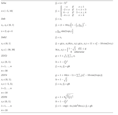
For the preliminary tests, two sets of functions, taken from the literature [14,15], were used and the perfor-mance of MACS was compared to the results in [14,15]. Therefore, for this set of tests, MTS was not included in the comparison. The function used in this section can be found in Table 1.

The first three functions were taken from reference [15]. Test cases Deb and Scha are two examples of disconnected Pareto fronts, Deb2 is an example of problem presenting multiple local Pareto fronts, 60 in this two-dimensional case.

The last three functions are instead taken from reference [14]. Test caseZDT2 has a concave Pareto front with a moderately high-dimensional search space. Test case ZDT6 has a concave Pareto front but because of the irregular nature of f1 there is a

strong bias in the distribution of the solutions. Test

case, ZDT4, with dimension 10, is commonly

Table 1 Multi-objective test functions

Scha f2¼(x5)2

x2[5, 10] f1¼

x if x1

2þx if 15x53

4x if 35x4

4þx if x44

8 > > < > > :

Deb f1¼x1

x1,x22[0, 1] f2¼ ð1þ10x2Þ

h

1 x1

1þ10x2

a¼2;q¼4 x1

1þ10x2sinð2qx1Þ

i

Deb2 f1¼x1

x12[0, 1] f2¼gðx1,x2Þhðx1,x2Þ;gðx1,x2Þ ¼11þx2210 cosð2x2Þ

x22[30, 30] hðx1,x2Þ ¼

n₁ ffiffiffif1 g

q

if f1g

0 otherwise

ZDT2 g¼1þ 9

n1

Pn

i¼2xi

xi2[0, 1]; h¼1 ðfg1Þ

2

i¼1,. . .,n f1¼x1;f2¼gh

n¼30

ZDT4 g¼1þ10ðn1Þ þPn_i¼2½x2

i 10 cosð2qxiÞ;

x12[0, 1]; h¼1

ffiffiffi

f1 g

q

xi2[5, 5]; f1¼x1;f2¼gh

i¼2,. . .,n

n¼10

ZDT6 g¼1þ9

ffiffiffiffiffiffiffiffiffiffiffiffiffi

Pn

i¼2xi n1

4

r

xi2[0, 1]; h¼1 ðfg1Þ

2

i¼1,. . .,n f1¼1exp(4x1)sin6(6px1);f2¼gh

recognized as one of the most challenging problems since it has 219different local Pareto fronts of which only one corresponds to the global Pareto-optimal front.

As a preliminary proof of the effectiveness of MACS, the average Euclidean distance of 500 uniformly spaced points on the true optimal Pareto front from the solutions stored in Ag by MACS was computed

and compared to known results in the literature. MACS was run 20 times to have a sample comparable to the one used for the other algorithms. The global archive was limited to 200 elements to be consistent with reference [14]. The value of the crowding factor wc, the thresholdtoland the convergenceminwere

kept constant to 1e-5 in all the cases to provide good local convergence.

To be consistent with reference [15], onDeb,Scha and, Deb2, MACS was run, respectively, for 4000, 1200, and 3200 function evaluations. Only two agents were used for these lower dimensional cases, with fe¼1/2. On test casesZDT2,ZDT4, and ZDT6,

MACS was run for a maximum of 25 000 function evaluations to be consistent with reference [14], with three agents and fe¼2/3 for ZDT2 and four

agents andfe¼3/4 onZDT4 andZDT6.

The results onDeb,Scha, andDeb2 can be found in Table 2, while the results onZDT2,ZDT4, andZDT6 can be found in Table 3.

On all the smaller dimensional cases, MACS per-forms comparably to MOPSO and better than PAES. It also performs than NSGA-II onDebandDeb2. On Scha, MACS performs apparently worse than NSGA-II, although after inspection one can observe that all the elements of the global archive Agbelong to the

Pareto front but not uniformly distributed, hence the higher value of the Euclidean distance. On the higher dimensional cases, MACS performs compara-bly to NSGA-II on ZDT2 but better than all the others on ZDT4 and ZDT6. Note, in particular, the improved performance on ZDT4.

On the same six functions, a different test was run to evaluate the performance of different variants of MACS. For all variants, the number of agents,fe,wc,

tol, and min was set as before, but instead of the

mean Euclidean distance, the success rates pconv

and pspr were measured for each variant. The

number of function evaluations for ZDT2, ZDT4, ZDT6, and Deb2 is the same as before, while for Scha and Deb it was reduced, respectively, to 600 and 1000 function evaluations given the good perfor-mance of MACS already for this number of function evaluations. Each run was repeated 200 times to have good confidence in the values ofpconvandpspr.

Four variants were tested and compared to the full version of MACS. Variant MACS no local does not

implement the individualistic moves and the local archive, variant MACSr¼1 has no adaptivity on the neighbourhood, its size is kept fixed to 1,variant MACS r¼0.1 has the size of the neighbourhood fixed to 0.1, variant MACS no attraction has the attraction mechanisms not active.

The result can be found in Table 4. The values of tolconvandtolsprare, respectively, 0.001 and 0.0035 for

ZDT2, 0.003 and 0.005 for ZDT4, 0.001 and 0.025 forZDT6, 0.0012 and 0.035 forDeb, 0.0013 and 0.04 forScha, 0.0015 and 0.0045 for Deb2. These thresh-olds were selected to highlight the differences among the various variants.

The table shows that the adaptation mechanism is beneficial in some cases although, in others, fixing the value ofrmight be a better choice. This depends on the problem and a general rule is difficult to derive at present. Other adaptation mechanisms could further improve the performance.

The use of individualistic actions coupled with a local archive is instead fundamental, so is the use of the attraction mechanism. Note, however, how the attraction mechanism penalizes the spreading on biassed problems like ZDT6, this is expected as it accelerates convergence.

Table 2 Comparison of the average Euclidean dis-tances between 500 uniformly space points on the optimal Pareto front for various opti-mization algorithms: smaller dimension test problems

Approach Deb2 Scha Deb

MACS 1.542e3 3.257e3 7.379e4

(5.19e4) (5.61e4) (6.36e5)

NSGA-II 0.094 644 0.001 594 0.002 536

(0.117 608) (0.000 122) (0.000 138)

PAES 0.259 664 0.070 003 0.002 881

(0.573 286) (0.158 081) (0.002 13)

MOPSO 0.001 161 1 0.001 473 96 0.002 057

(0.000 720 5) (0.000 201 78) (0.000 286)

Table 3 Comparison of the average Euclidean dis-tances between 500 uniformly space points on the optimal Pareto front for various opti-mization algorithms: larger dimension test problems

Approach ZDT2 ZDT4 ZDT6

MACS 9.0896e4 0.0061 0.0026

(4.0862e5) (0.0133) (0.0053)

NSGA-II 0.000 824 0.513 053 0.296 564

(<1e5) (0.118 460) (0.013 135)

PAES 0.126 276 0.854 816 0.085 469

4.4. Application to space trajectory design

In this section, we present the application of MACS to three space trajectory problems: a two-impulse orbit transfer from a low Earth orbit (LEO) to a high-eccen-tricity Molniya-like orbit, a three-impulse transfer from a LEO to geostationary Earth orbit (GEO) and a multi gravity assist transfer to Saturn equivalent to the transfer trajectory of the Cassini mission. The first two cases are taken from the work of Minisci and Avanzini [7].

In the two-impulse case, the spacecraft departs at time t0 from a circular orbit around the Earth (the

gravity constant is E¼3.986 0105km3/s2) with

radiusr0¼6721 km and at timetfis injected into an

elliptical orbit with eccentricityeT¼0.667 and

semi-major axis aT¼26 610 km. The transfer arc is

com-puted as the solution of a Lambert’s problem [20] and the objective functions are the transfer time T¼tft0and the sum of the two norms of the velocity

variations at the beginning and at the end of the transfer arc vtot. The objectives are functions of

the solution vector x¼[t0 tf]T2D R2. The search

space D is defined by the following intervals t02[0

10.8] andtf2[0.03 10.8].

In the three-impulse case, the spacecraft departs at time t0 from a circular orbit around the Earth with

radius r0¼7000 km and after a transfer time

T¼t1þt2is injected into a circular orbit with radius

rf¼42 000. An intermediate manoeuvre is performed

at timet0þt1and at position defined in polar

coordi-nates by the radiusr1and the angley1. The objective

functions are the total transfer timeTand the sum of the three impulsesvtot. The solution vector in this

case isx¼[t0,t1,r1,y1,tf]T2D R5. The search space

D is defined by the following intervals t02[0 1.62],

t12[0.03 21.54], r12[7010 105410], y12[0.01

2p0.01], andt22[0.03 21.54].

The Cassini case consists of five transfer arcs con-necting a departure planet, the Earth, to the destina-tion planet, Saturn, through a sequence of swing-by’s with the planets: Venus, Venus, Earth, and Jupiter. Each transfer arc is computed as the solution of a

Lambert’s problem [21] given the departure time from planet Pi and the arrival time at planet Piþ1.

The solution of the Lambert’s problems yields the required incoming and outgoing velocities at each swing-by planetvinandvrout. The swing-by is

mod-elled through a linked-conic approximation with powered manoeuvres [22], i.e. the mismatch between the required outgoing velocityvroutand the

achiev-able outgoing velocityvaoutis compensated through a

vmanoeuvre at the pericentre of the gravity assist hyperbola. The whole trajectory is completely defined by the departure timet0and the transfer time for each

legTi, withi¼1,. . ., 5. The normalized radius of the

pericentrerp,i of each swing-by hyperbola is derived

a posteriorionce each powered swing-by manoeuvre is computed. Thus, a constraint on each pericentre radius has to be introduced during the search for an optimal solution. In order to take into account this constraint, one of the objective functions is aug-mented with the weighted violation of the constraints

f ðxÞ ¼v0þ

X4

i¼1

viþvf þ

X4

i¼1

wiðrp,irpmin,iÞ2

ð16Þ

for a solution vectorx¼[t0, T1, T2,T3, T4,T5]T. The

objective functions are, the total transfer time T ¼P5_i Ti andf(x). The minimum normalized

peri-centre radii are rpmin,1¼1.0496, rpmin,2¼1.0496,

rpmin,3¼1.0627, and rpmin,4¼9.3925. The search

space D is defined by the following intervals: t02[1000, 0]MJD2000, T12[30, 400]d, T22[100,

470]d, T32[30, 400]d, T42[400, 2000]d, and

T52[1000, 6000]d. The best known solution for

the single objective minimization of f(x) is fbest¼4.9307 km/s, with xbest¼[789.753, 158.2993,

449.3859, 54.7060, 1024.5896, 4552.7054]T.

4.4.1 Test results

For this second set of tests, each algorithm was run for the same number of function evaluations. In partic-ular, consistent with the tests performed in the work

Table 4 Comparison of different versions of MACS

Approach Metric ZDT2(%) ZDT4(%) ZDT6(%) Scha(%) Deb(%) Deb2(%)

MACS pconv 83.5 75 77 73 70.5 60

pspr 22.5 28 58.5 38.5 83 67.5

MACS pconv 14 0 45 0.5 72.5 11

no local pspr 1 0 34 0 4 15

MACS pconv 84 22 78 37 92 21

r¼1 pspr 22 7 63 0 54 38

MACS pconv 56 42 57 78 85 42

r¼0.1 pspr 5 15 61 88 94.5 74

MACS pconv 21 0.5 14.5 0.5 88.5 0

of Minisci and Avanzini [7], we used 2000 function evaluations for the two-impulse case and 30 000 for the three-impulse case. For the Cassini case, instead, the algorithms were run for 180 000, 300 000, and 600 000 function evaluations.

Note that the version of all the algorithms used in this second set of tests is the one that is freely avail-able online, written in C/Cþþ. We tried in all cases to stick to the available instructions and recommenda-tions by the author to avoid any bias in the comparison.

The threshold values for the two-impulse cases was taken from reference [7] and is tolconv¼0.1,

tolspr¼2.5. For the three-impulse, case instead we

considered tolconv¼5.0, tolspr¼5.0. For the Cassini

case, we usedtolconv¼0.75,tolspr¼5, instead. These

values were selected after looking at the dispersion of the results over 200 runs. Lower values would result in a zero value of the performance indexes of all the algorithms, which are not very significant for a comparison.

MACS was tuned on the three-impulse case. In par-ticular, the crowding factorwc, the thresholdrtoland

the convergence rmin were kept constant to 1e5,

which is below the required local convergence accu-racy, whilefeandnpopwere changed. A value of 1e-5 is

expected to provide good local convergence and good density of the samples belonging to the Pareto front. Table 5 reports the value of performance indexes

pconvandpsprover 200 runs of MACS with different

settings. The indexpsprand the indexpconvhave

dif-ferent, almost opposite, trends. However, it was decided to select the setting that provides the best convergence,i.e. npop¼15 and fe¼1/3. This setting

will be used for all the tests in this article.

On top of the complete algorithm, two variants of MACS were tested: one without individualistic moves and local archive, denoted asno localin the tables, and one with no attraction towards the global archive Ag, denoted as no att in the tables. Only these two

variants are tested on these cases as they displayed the most significant impact in the previous standard test cases and more importantly were designed spe-cifically to improve performances.

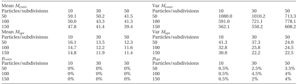
NSGA-II, PAES, MOPSO, and MTS were tuned as well on the three-impulse case. In particular, for NSGA-II the best result was obtained for 150 individ-uals and can be found in Table 6. A similar result could be obtained for MOPSO (Table 7). For MTS, only the population was changed while the number of individuals performing local moves was kept con-stant to 5. The results of the tuning of MTS can be found in Table 8. For the tuning of PAES the results can be found in Table 9.

All the parameters tuned in the three-impulse case were kept constant except for the population size of NSGA-II and MOPSO. The size of the population of NSGA-II and MOPSO was set to 100 and 40, respec-tively, on the two impulse case and was increased with the number of function evaluations in the Cassini case. In particular, for NSGA-II, the following ratios between population size and number of func-tion evaluafunc-tions were used: 272/180 000, 353/300 000, and 500/600 000. For MOPSO, the following ratios between population size and number of function evaluations were used: 224/180 000, 447/300 000, and 665/600 000. This might not be the best way to set the population size for these two algorithms, but it

Table 5 Indexespconvandpsprfor different settings of

MACS on the three-impulse case

npop(%)¼5 npop(%)¼10 npop(%)¼15

pconv

fe¼1/3 45.5 55.5 61.0

fe¼1/2 48.0 51.0 55.5

fe¼2/3 45.0 52.5 43.0

pspr

fe¼1/3 68.5 62.0 56.0

fe¼1/2 65.0 57.0 46.0

fe¼2/3 67.5 51.0 36.5

Table 6 NSGAII tuning on the three-impulse case

MeanMconv VarMconv

Zc/Zm 5 25 50 Zc/Zm 5 25 50

5 36.1 38.3 43.0 5 201.0 202.0 185.0

10 32.3 39.4 40.6 10 182.0 172.0 182.0

20 31.7 39.6 42.5 20 175.0 183.0 169.0

MeanMspr VarMspr

Zc/Zm 5 25 50 Zc/Zm 5 25 50

5 6.77 7.24 8.08 5 9.97 9.47 7.25

10 5.91 7.50 7.81 10 9.74 8.68 8.34

20 5.78 7.50 8.16 20 9.75 8.53 8.04

pconv pspr

Zc/Zm 5 25 50 Zc/Zm 5 25 50

5 0.0% 0.0% 0.0% 5 44.8% 37.7% 23.4%

10 0.0% 0.0% 0.0% 10 57.8% 33.1% 29.2%

is the one that provided better performance in these tests.

Note that the size of the global archive for MACS was constrained to be lower than the size of the pop-ulation of NSGA-II, in order to avoid any bias in the computation ofMspr.

The performance of all the algorithms on the Cassini case can be found in Table 10 for a variable number of function evaluations.

For the three-impulse case, MACS was able to iden-tify an extended Pareto front (Figs 2(a) and (b)), where all the non-dominated solutions from all the 200 runs are compared to the global front), compared to the results in reference [7]. The gap in the Pareto front is probably due to a limited spreading of the solutions in that region. Note the cusp due the transition between

the condition in which two-impulse solutions are optimal and the condition in which three-impulse solutions are optimal.

Table 10 summarizes the results of all the tested algorithms on the two-impulse case. The average value of the performance metrics is reported with, in parentheses, the associated variance over 200 runs. The two-impulse case is quite easy and all the algorithms have no problems identifying the front. However, MACS displays a better convergence than the other algorithms, while the spreading of MOPSO and MTS is superior to the one of MACS.

The three-impulse case is instead more problem-atic (Table 11). NSGA-II is not able to converge to the upper-left part of the front and therefore the conver-gence is 0 and the spreading is comparable to the one

Table 7 MOPSO tuning on the three-impulse case

MeanMconv VarMconv

Particles/subdivisions 10 30 50 Particles/subdivisions 10 30 50

50 59.1 50.2 41.5 50 1080.0 1010.2 713.3

100 50.0 43.3 41.3 100 591.0 721.1 778.1

150 47.8 41.4 39.4 150 562.1 550.2 608.2

MeanMspr VarMspr

Particles/subdivisions 10 30 50 Particles/subdivisions 10 30 50

50 16.1 13.5 12.3 50 41.3 37.3 24.0

100 14.7 12.2 11.6 100 32.8 25.8 24.5

150 14.8 11.9 11.4 150 30.0 22.2 22.5

pconv pspr

Particles/subdivisions 10 30 50 Particles/subdivisions 10 30 50

50 0% 0% 0% 50 0.5% 2.5% 3.5%

100 0% 0% 0% 100 0.5% 4.5% 4%

150 0% 0% 0% 150 0.5% 2% 4%

Table 8 MTS tuning on the three-impulse

3imp Population 20 40 80

Mconv Mean 17.8 22.6 23.6

Var 97.6 87.8 73.2

Mspr Mean 12.6 19.9 18.4

Var 34.7 26.2 18.6

pconv 1.0% 0.0% 0.0%

pspr 0.5% 0.0% 0.0%

Table 9 PAES tuning on the three-impulse case

MeanMconv VarMconv

Subdivisions/mutation 0.6 0.8 0.9 Subdivisions/mutation 0.6 0.8 0.9

1 53.7 70.6 70.2 1 525.0 275.0 297.0

2 52.8 70.2 70.0 2 479.0 266.0 305.0

4 53.0 70.2 70.1 4 453.0 266.0 311.0

MeanMspr VarMspr

Subdivisions/mutation 0.6 0.8 0.9 Subdivisions/mutation 0.6 0.8 0.9

1 14.2 27.7 36.7 1 20.0 14.3 17.3

2 13.6 27.6 36.6 2 17.5 14.6 16.8

4 13.8 27.7 36.6 4 17.2 15.8 17.0

pconv pspr

Subdivisions/mutation 0.6 0.8 0.9 Subdivisions/mutation 0.6 0.8 0.9

1 0.0% 0.0% 0.0% 1 0.0% 0.0% 0.0%

2 0.0% 0.0% 0.0% 2 0.0% 0.0% 0.0%

of MACS. All the other algorithms perform poorly with a value of almost 0 for the performance indexes.

This is mainly due to the fact that no one can identify the vertical part of the front.

Note that the long tail identified by NSGA-II is actu-ally dominated by two points belonging to the global front (Fig. 2(b)).

Table 12 reports the statistics for the Cassini prob-lem. On top of the performance of the three variants tested on the other two problems, the table reports also the result for 10 agents andfe¼5. For all numbers

of function evaluations, MACS has better spreading than NSGA-II, because NSGA-II converges to a local Pareto front. Nonetheless, NSGA-II displays a more regular behaviour and a better convergence for low number of function evaluations although it never reaches the best front. The Pareto fronts are repre-sented in Figs 3(a) and (b) (even in this case, the figures represent all the non-dominated solutions coming from all the 200 runs). Note that, the minimum f returned by MACS is the best known solution for the single objective version of this problem [9]. All the other algorithms perform quite poorly on this case.

Of all the variants of MACS tested on these prob-lems, the full complete one is performing the best. As expected, in all three cases, removing the individual-istic moves severely penalizes both convergence and spreading. It is interesting to note that removing the attraction towards the global front is also compara-tively bad. On the two-impulse case, it does not impact the spreading but reduces the convergence, while on the Cassini case, it reduces mean and vari-ance but the success rates are zero. The observable reason is that MACS converges slower but more uni-formly to a local Pareto front.

Finally, it should be noted that mean and variance seem not to capture the actual performance of the

0 50 100 150 200 250 300 350

0 5 10 15 20 25 30

Pareto Front Comparison (a)

(b)

Δ v tot [km/s]

T [h]

Global MACS NSGA−II

Part of the front not identified by NSGAII

Dominated tail

10 20 30 40 50 60

0 1 2 3 4 5 6 7 8

Pareto Front Comparison

Δ v tot [km/s]

T [h]

Global MACS NSGA−II

Dominated tail

Fig. 2 Three-impulse test case: (a) complete Pareto front, (b) close-up of the Pareto fronts

Table 10 MetricsMconvandMspr, and associated performance indexespconvandpspr, on

the two impulse test cases

Metric MACS MACS no local MACS no att NSGA-II PAES MOPSO MTS

Mconv 0.0077 0.039 0.0534 0.283 0.198 0.378 0.151

(1e-3) (1.4e-2) (9.5e-3) (4.35e-3) (0.332) (0.0636) (0.083)

Mspr 2.89 6.87 3.08 2.47 332.0 2.11 1.95

(0.49) (7.36) 0.943 (0.119) (2.61e4) (2.65) (1.41)

pconv 98.5% 91.5% 84% 0% 75.5% 9% 57.5%

pspr 29.5% 0% 24% 62.5% 0.5% 94.5% 85.5%

Table 11 Summary of metricsMconvandMspr, and associated performance indexespconv

andpspr, on the three impulse test cases

Metric MACS MACS no local MACS no att NSGA-II PAES MOPSO MTS

Mconv 5.53 7.58 154.7 31.7 53.0 39.4 17.8

(15.1) (26.3) (235.0) (175.0) (453.0) (608.1) (97.6)

Mspr 5.25 6.03 9.16 5.78 13.8 11.4 12.6

(3.73) (3.95) (2.07) (9.75) (17.2) (22.5) (34.7)

pconv 61.0% 40.5% 0.0% 0.0% 0.0% 0% 1.0%

algorithms. In particular, they do not capture the abil-ity to identify the whole Pareto front as the success rates instead do.

5. CONCLUSIONS

In this article, we presented a hybrid evolutionary algorithm for multi-objective optimization problems. The effectiveness of the hybrid algorithm, imple-mented in a code called MACS, was demonstrated at first on a set of standard problems and then its performance was compared against NSGA-II, PAES, MOPSO, and MTS on three space trajectory design problems. The results are encouraging as, for the same computational effort (measured in number of function evaluations, MACS was converging more accurately than NSGA-II on the two-impulse case and managed to find a previously undiscovered part of the Pareto front of the three-impulse case. As a consequence, on the three-impulse case, MACS, has better performance metrics than the other algo-rithms. On the Cassini case, NSGA-II appears to con-verge better to some parts of the front although MACS yielded solutions with better f and identifies once

more a part of the front that NSGA-II cannot attain. PAES and MTS do not perform well on the Cassini case, while MOPSO converges well locally but, with the settings employed in this study, yielded a very poor spreading.

From the experimental tests in this article, we can argue that the following mechanisms seem to be par-ticularly effective: the use of individual local actions with a local archive as they allow the individuals to move towards and within the Pareto set; the use of an attraction mechanism as it accelerates convergence.

Finally, it should be noted that all the algorithms tested in this study use the Pareto dominance as selection criterion. Different criteria, like the decom-position in scalar subproblems, can be equality implemented in MACS, without disrupting its work-ing principles, and lead to different performance results.

ACKNOWLEDGEMENTS

The authors would like to thank Dr Edmondo Minisci and Dr Guilio Avanzini for the two-and three-impulse cases and the helpful advice.

0 50 100 150 200 250

1000 2000 3000 4000 5000 6000 7000

Pareto Front Comparison

(a)

(b)

f [km/s]

T [day]

Global MACS NSGA−II

4 5 6 7 8 9 10

2000 2500 3000 3500 4000 4500 5000 5500 6000

Pareto Front Comparison

f [km/s]

T [day]

Global MACS NSGA−II

Fig. 3 Cassini test case: (a) complete Pareto front and (b) close-up of the Pareto fronts

Table 12 MetricsMconvandMspr, and associated

per-formance indexes pconv and pspr, on the

Cassini case

Approach Metric 180k 300k 600k

MACS 5/15 Mconv 6.50 (229.1) 4.48 (107.1) 3.91 (62.6)

Mspr 12.7 (126.0) 11.1 (83.1) 8.64 (35.5)

pconv 6% 14% 21.5%

pspr 27.5% 31% 41%

MACS 5/10 Mconv 6.74 (217.9) 5.56 (136.4) 3.14 (50.1)

Mspr 12.1 (83.0) 10.3 (63.7) 8.11 (30.0)

pconv 8% 10% 25.5%

pspr 26.0% 31.5% 45.5%

MACS no local Mconv 13.5 (436.2) 10.2 (350.1) 7.86 (190.2)

Mspr 31.1 (274.3) 27.9 (278.9) 21.9 (226.7)

pconv 1.0% 1.5% 2.5%

pspr 1.0% 2.5% 6%

MACS no att Mconv 2.62 (1.46) 2.2 (0.88) 1.82 (0.478)

Mspr 27.8 (83.2) 22.9 (58.0) 18.2 (28.0)

pconv 0.0% 0.0% 1.0%

pspr 0.0% 0.0% 0.0%

NSGA-II Mconv 2.43 (18.0) 1.99 (16.8) 1.24 (1.62)

Mspr 11.6 (71.4) 11.0 (47.5) 8.78 (28.2)

pconv 17.5% 24.0% 29.0%

pspr 15.5% 12.5% 25.0%

MOPSO Mconv 2.62 (7.33) 2.4 (2.57) 2.14 (0.94)

Mspr 28.0 (308.3) 24.6 (260.4) 21.8 (231.3)

pconv 0.5% 1.0% 1.0%

pspr 0.0% 0.0% 0.5%

PAES Mconv 24.0 (54.5) 19.8 (32.9) 15.2 (16.6)

Mspr 30.1 (47.3) 26.0 (33.9) 21.4 (19.5)

pconv 0.0% 0.0% 0.0%

pspr 0.0% 0.0% 0.0%

MTS Mconv 3.71 (1.53) 3.39 (1.67) 3.02 (1.69)

Mspr 18.1 (18.2) 15.6 (13.4) 13.1 (8.46)

pconv 0.0% 0.0% 0.0%

ßAuthors 2011

REFERENCES

1 Coverstone-Caroll, V., Hartmann, J. W., and

Mason, W. M. Optimal multi-objective low-thrust spacecraft trajectories. Compu. Methods Appl. Mech. Eng., 2000,186, 387–402.

2 Dachwald, B. Optimization of interplanetary solar sailcraft trajectories using evolutionary neurocon-trol.J. Guid. Dyn., 2004,27, 66–72.

3 Lee, S., von Allmen, P., Fink, W., Petropoulos, A. E.,

andTerrile, R. J.Multiobjective evolutionary algo-rithms for low-thrust orbit transfer optimization. In Proceedings of the Genetic and Evolutionary

Computation Conference (GECCO 2005),

Washington DC, USA, 25–29 June 2005.

4 Schu¨tze, O., Vasile, M. M.,andCoello Coello, C. A.

Approximate solutions in space mission design. In Parallel Problem Solving from Nature (PPSN 2008), Dortmund, Germany, 13–17 September, 2008.

5 Schu¨tze, O., Vasile, M., Junge, O., Dellnitz, M.,and

Izzo, D.Designing optimal low-thrust gravity-assist trajectories using space pruning and a multi-objec-tive approach.Eng. Optim., 2009,41(2), 155–181.

6 Dellnitz, M., Ober-Blbaum, S., Post, M., Schtze, O.,

and Thiere, B. A multi-objective approach to the design of low thrust space trajectories using optimal control. Celestial Mech. Dyn. Astron., 2009,105(1), 33–59.

7 Minisci, E. andAvanzini, G. Optimisation of orbit transfer manoeuvres as a test benchmark for evolu-tionary algorithms. In Proceedings of the 2009 IEEE Congress on Evolutionary Computation (CEC2009), Trondheim, Norway, May 2009, pp. 350–357.

8 Vasile, M. A behavioral-based meta-heuristic for robust global trajectory optimization. In Proceedings

of the 2007 IEEE Congress on Evolutionary

Computation (CEC2007), Singapore, September 2007, pp. 2056–2063.

9 Vasile, M. and Locatelli, M. A hybrid multiagent approach for global trajectory optimization. J. Global Optim., 2009,44(4), 461–479.

10 Adriana Lara, Gustavo Sanchez, Carlos A. Coello Coello, and Oliver Schu¨tze. HCS: A new local search strategy for memetic multi-objective evolu-tionary algorithms. IEEE Trans. Evol. Comput., 2010,14(1), 112–132.

11 Zhang, Q.andLi, H.Moea/d: A multi-objective evo-lutionary algorithm based on decomposition. IEEE Trans. Evol. Comput., 2007,11(6), 712–731.

12 Price, K. V., Storn, R. M., and Lampinen, J. A.

Differential evolution. A practical approach to global optimization, 2005 (Natural Computing Series, Springer, Berlin).

13 Vasile, M. and Zuiani, F. A hybrid multi-objective optimization algorithm applied to space trajectory optimization. In Proceedings of the IEEE International Conference on Evolutionary

Computation, Barcelona, Spain, July 2010,

pp. 308–315.

14 Deb, K. A., Pratap, A.,andMeyarivan, T.Fast elitist multi-objective genetic algorithm: Nga-ii. Kangal report no. 200001, KanGAL, 2000.

15 Coello, C.andLechuga, M.Mopso: A proposal for multiple objective particle swarm optimization. Technical report evocinv-01-2001., CINVESTAV, Instituto Politecnico Nacional Col, San Pedro Zacatenco, Mexico, 2001.

16 Knowles, J. D.andCorne, D. W.The pareto archived evolution strategy: A new baseline algorithm for pareto multi-objective optimisation. In Proceedings

of the IEEE International Conference on

Evolutionary computation, Washington DC, US, 1999, pp. 98–105.

17 Tseng, L.-Y.andChen, C.Multiple trajectory search for multi-objective optimization. In Proceedings of the IEEE International Conference on Evolutionary computation, Singapore, 25–28 September 2007, pp. 3609–3616.

18 Van Veldhuizen, D. A. and Lamont, G. B.

Evolutionary computation and convergence to a pareto front. In Late Breaking papers at the Genetic Programming, California, July 1998, pp. 221–228.

19 Vasile, M., Minisci, E.,andLocatelli, M.On testing global optimization algorithms for space trajectory

design. In Proceedings of the AIAA/AAS

Astrodynamic Specialists Conference Honolulu, Hawaii, USA, August 2008.

20 Avanzini, G. A simple Lambert algorithm. J. Guidance, Control, Dynamics, 2008, 31(6), 1587–1594.

21 Battin, R.An Introduction to the mathematics and methods of astrodynamics., 1999 (AIAA).

22 Myatt, D. R., Becerra, V. M., Nasuto, S. J., and

Bishop, J. M.Global optimization tools for mission analysis and design.2004, Final rept. esa ariadna itt ao4532/18138/04/nl/mv,call03/4101, ESA/ESTEC.

APPENDIX

Notation

aT semimajor axis

Ag global archive

Al local archive

D search space

eT eccentricity

f cost function

fe fraction of the population doing local

moves

Id dominance index

Mconv convergence metrics

Mspr spreading metrics

neval number of function evaluations

npop population size

Nr neighbourhood of solutionx

Ne maximum number of allowed function

pconv percentage of success on convergence

pspr percentage of success on spreading

Pi ith planet

Pk population at generationk

r random number

rp pericentre radius

rpmin minimum pericentre radius

s resource index

S selection function

t0 departure time

ti manoeuvre time

tf final time

T transfer time

u variation of the solutionx

U uniform distribution

wc tolerance on the maximum allowable

crowding

x solution vector

X Pareto optimal set

y mutate individual

v variation of velocity

yi true anomaly of manoeuvrei

E gravity constant