Integration of a mean-torque diesel engine model into a
hardware-in-the-loop shipboard network simulation using
lambda-tuning
A. J. Roscoe*, I. M. Elders*, J. E. Hill†, G. M. Burt*
*Institute for Energy and Environment, University of Strathclyde, Glasgow, G1 1XW [email protected]
†Rolls-Royce plc, Derby, UK
Keywords: marine electrical systems/technologies, power system control, power system stability, power system reliability, simulation.
Abstract
This paper describes the creation of a hardware-in-the-loop (HIL) environment for use in evaluating network architecture, control concepts and equipment for use within marine electrical systems. The environment allows a scaled hardware network to be connected to a simulation of a multi-megawatt marine diesel prime-mover, coupled via a synchronous generator. This allows All-Electric marine scenarios to be investigated without large-scale hardware trials. The method of closing the loop between simulation and hardware is described, with particular reference to the control of the laboratory synchronous machine which represents the simulated generator(s). The fidelity of the HIL simulation is progressively improved in this paper. Firstly a faster and more powerful field drive is implemented to improve voltage tracking. Secondly the phase tracking is improved by using two nested PIDA (proportional integral derivative acceleration) controllers for torque control, tuned using lambda-tuning. The HIL environment is tested using a scenario involving a large constant-power load step. This both provides a very severe test of the HIL environment, and also reveals the potentially adverse effects of constant-power loads within marine power systems.
1 Introduction
meet the existing and forthcoming standards of reliability and safety, as well as delivering the promised benefits in maintainability and reduced fuel use.
One approach that has been adopted in meeting this challenge is the construction of a full-scale hardware demonstrator [1]. While this approach has obvious advantages, it also has several drawbacks, including high costs, limited flexibility, and the inability to evaluate equipment at the design stage. Alternatively, evaluation of designs through simulation can be adopted, which removes some of the cost and inflexibility of an all-hardware approach, but requires sufficiently accurate models of all components which are to be included. Where equipment or phenomena are poorly understood or poorly documented, this can be a significant barrier.
A third approach is to adopt a reduced-scale Hardware-in-the-Loop (HIL) approach [2] [3] [4] [5] [6] in which physical machines, drives, cables, etc. are used to represent certain parts of the system, while others are represented using simulation models. Key advantages of this approach, which is described in more detail in [7], include the ability to evaluate the actual performance of physical drives, controllers, etc., as well as the option to scale the output from large simulated devices such as prime movers in a way which would not be possible in hardware.
This paper describes the adaption and integration of a model of a large multi-megawatt diesel engine, as developed by the manufacturer, into a kilowatt-scale marine network hardware demonstrator. To improve the fidelity of the HIL experiments, pre-existing laboratory HIL capability described in [7] is augmented; firstly with more powerful field controls, and secondly using a dual nested control loop using PIDA controllers, which are tuned in turn using the “Iambda tuning” approach. To demonstrate the effectiveness of the approach, measurements of the HIL network behaviour are compared with equivalent simulations. The test scenario used is a large constant-power load step. It is shown that good agreement in both electrical and mechanical behaviour can achieved in the HIL simulation.
2 Choice of test scenario: constant power load step
calculations, the propeller characteristic (torque as a function of propeller speed) can be approximated as a square-law in the first quadrant, i.e. the propeller pushing the vessel through the water in the forward direction.
At low vessel speeds, it is usual to control the propeller at a constant speed via a propulsion motor speed-control loop. However, at higher vessel speeds, the response of this type of control scheme is unsatisfactory. Small changes in vessel speed, due to a dynamic change in vessel resistance, lead to large changes in the torque (and electrical power demand) demanded via the propulsion motors. This in turn leads to changes in electrical system frequency, and is particularly problematic at higher sea states. The electrical generators are governed to maintain constant frequency, and therefore the engine fuel demand also fluctuates. Overall, this causes extra stress and wear on the prime movers. Therefore, a constant-power propulsion mode is used at higher vessel speeds. Changes in the vessel resistance are then manifest through changes in the vessel speed which are smoothed through the vessel’s inertia, which is usually large.
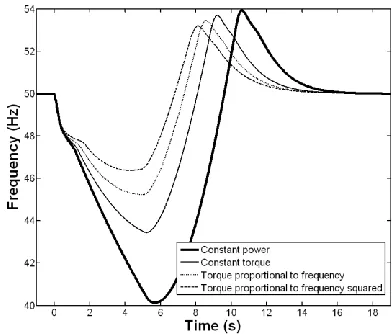
In modern vessels with an All-Electric design, such constant-power drive systems are relatively easy to implement, using power electronics. However, the impact that a step change in load applied through a constant-power drive can have on a marine power system is large. As an illustration, Fig. 1 and Fig. 2 show the resulting generator torque and frequency (speed) from four different load steps of 0.5pu (per-unit):
Constant power of 0.5 pu
Constant torque of 0.5 pu
Torque proportional to electrical frequency
Torque proportional to electrical frequency squared
Clearly, the constant-power load step causes the biggest perturbation to the power system. This is because the torque at the generator shaft is inversely dependent upon engine speed, for a given power, and therefore rises as the frequency (engine speed) falls, exacerbating the frequency dip. Sudden introductions of loads in constant torque mode, or where torque falls when speed (frequency) falls, provide much smaller perturbations.
1500rpm, giving 50Hz). The inputs to the engine model are the speed reference (set to an un-drooped value of 1pu for a 50Hz target), and the generator torque. The per-unit torque is calculated by the per-unit load power divided by the per-unit frequency. Two cases of this scenario are presented and compared. In the first case (“Pure Simulation”), the engine model plus the electrical load are simulated. In this case, the electrical load is set to a perfect step-function. In the second case, (“HIL”), the engine model is simulated, but the electrical load is applied in hardware using a resistive loadbank, The loadbank is insensitive to frequency, and therefore, so long as the system voltage remains at 1pu, the resistive load behaves as a constant-power load. In both cases, it is assumed that the generator maintains a constant 1pu voltage during the step, due to effective AVR action. In reality, an actual AVR may struggle to maintain nominal voltage during the severe test presented in this study, in the same way that the HIL hardware cannot reduce voltage excursions to exactly zero. However, the assumption of perfect regulation is useful because it provides both the harshest tests of the diesel engine and the HIL hardware, and also it allows simple frequency-insensitive resistive loadbanks to be used in hardware to provide the constant-power load step.
In the hardware (HIL) test, the diesel engine model (which models a machine at the 4 MW scale) was scaled such that its nominal 1pu power rating was 37.4kW. Thus, the actual resistive load applied was nominally a resistive 18.7kW (0.5 pu) at 400V (1pu), 3-phase, 50Hz. The scaling to the multi-MW model is achieved in this case by simply multiplying the measured electrical power flow in hardware by the factor 4000/37.4, to derive the power (and hence torque via knowledge of the rotational speed) which would have been extracted from the full-scale diesel.
3 Architecture of simulation and HIL implementation
3.1 Simulation of diesel engine
The mean-torque diesel engine model used in this paper is a significant piece of proprietary MATLAB® Simulink® code, supplied by a European manufacturer of marine reciprocating engines. The structure of this simulation model approximately follows that described in [9]. A simpler model, developed specifically for HIL applications, is presented in [10].
magnetic phenomena or the electrical behaviour of the generator; the electrical behaviour is determined by the physical synchronous generator.
The diesel model was originally developed in the “continuous” mode within Simulink, and so this has been converted for use with discrete simulations (and HIL applications) by replacing all filters, differentials and integrals with digital equivalents. For this paper, a time step of 2ms is used, since it matches that used in the HIL application.
3.2 Hardware in the loop implementation
The diesel engine model can be placed within a HIL environment (Fig. 3). In this case, the aim is to control a real 80kVA synchronous motor-generator so that it behaves with the same speed/torque and inertial response as the model of the diesel engine and coupled generator. This allows an entire laboratory network of loads, interconnectors, breakers, and smaller generators to be connected. The power hardware network can thus virtually driven by the model of the diesel/generator, and the model of the diesel/generator becomes loaded by the network. The closure of this feedback loop creates a HIL environment. It should be noted that while this paper refers specifically to scenarios where the simulated part consists of a diesel reciprocating engine, the hardware-in-the-loop design, functionality and fidelity is applicable to many other types of simulated prime movers, machines or electrical networks. When entire electrical networks are required to be simulated, an appropriate electrical real-time simulator is required [7].
The 80kVA motor-generator is driven by a fast responding DC motor coupled to a thyristor drive. The essential details of this implementation are described in [7]. However, in this case the simulation of the diesel engine can be executed on the same computer as the HIL control (the simulator and controller in Fig. 3). Also, the diesel engine model returns a speed output as a response to a torque input, and this speed output must be integrated to provide the phase of VN*. This integration includes an arbitrary (constant) phase offset value which is essentially a free
variable. For these two reasons, so long as the sampled values of VN, IN are measured carefully with matched
anti-aliasing filters and made coherently (or processed to be coherent as in [7]), then there is essentially zero loop delay. This significantly simplifies the implementation compared to previous work in [7].
4 Incremental improvements to HIL fidelity
and the torque control used a control algorithm shown in Fig. 2 of [7]. It was shown in [7] that although the rotary exciter had sufficient power to maintain steady-state operation, it was lacking in sufficient overhead voltage capability to enable the toughest HIL scenarios to be tracked accurately. This is borne out in the first set of results, shown in Fig. 4, and by the “original” lines on Fig. 11 to Fig. 13. In particular, the poor voltage tracking (Fig. 11) leads to a drop in power flow relative to the pure simulation
4.1 Improving the accuracy of the voltage tracking at the shared node
To improve the voltage tracking, the rotary exciter for the 80kVA generator was removed from the HIL hardware, and replaced with a large solid-state DC power supply with a high switching frequency and fast response. This has adequate DC current capability to maintain steady-state terminal voltage at the machine rating. More significantly, it has a much higher available DC voltage than the rotary exciter. This enables the field current to be increased much more rapidly during load changes, allowing terminal voltage to be regulated much better. The particular DC supply used during this study is only capable of generating positive voltages. For the scenario presented, this is acceptable. For scenarios involving tracking of voltage dips, a bidirectional DC source capable of negative voltage output and reverse power flow would be highly desirable, to allow forcible collapse of the field. The field control contains a PID (proportional-integral-derivative) controller, and the control gains can be increased using the DC supply, due to the faster response of the field using this hardware.
Using the improved field control leads to the dashed lines on Fig. 11 to Fig. 13. Notably, the voltage tracking error is much reduced, and therefore the power flow in the HIL experiments is much closer to the “pure simulation” case, than with the original setup.
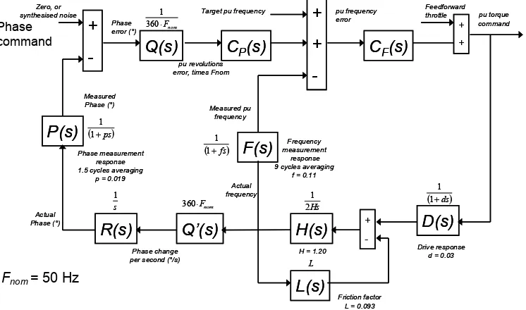
4.2 Improving the accuracy of the phase tracking at the shared node
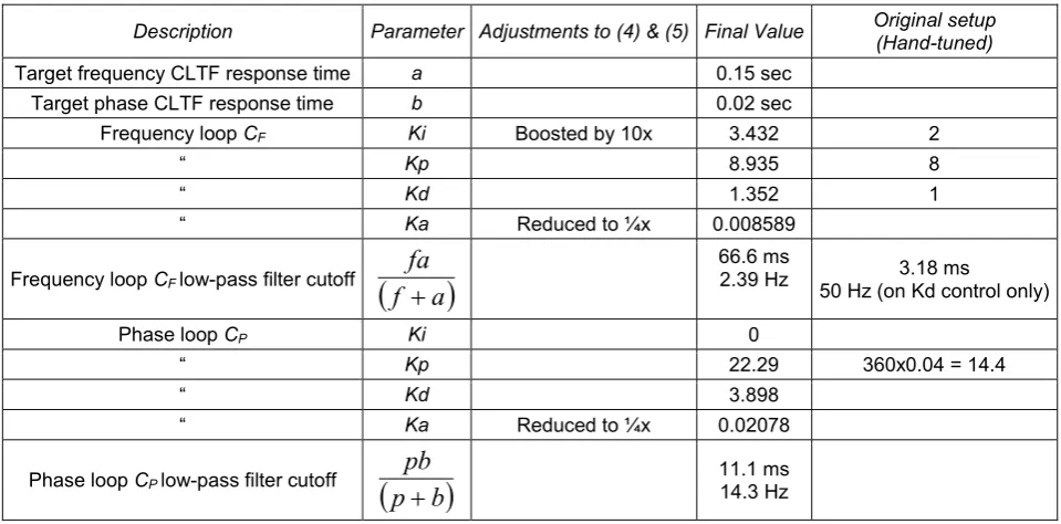
In [7], the torque control to the DC motor (driving the 80kVA generator) was derived using a phase-locking control shown in Fig. 2 of [7]. This consisted of a PID controller to control frequency, using an additional low-pass filter on the differential control (only) to limit the effects of measurement noise [11], augmented with a simple proportional-only controller to enable tracking of phase. In addition, the values of the control parameters were obtained by hand tuning in the laboratory. The values of these original parameters are shown in Table 1.
tests, such as spin-down tests (to measure inertia and friction), and step-changes in command torque (to measure drive response). Knowledge of these parameters, combined with knowledge of the measurement algorithms, allows the system to be modelled to the required level of accuracy. The model structure is shown in Fig. 5.
The right-hand loop of Fig. 5 is a conventional loop for controlling frequency to a given target. The left-hand loop augments the control system with the unconventional (but required) control of generator phase to achieve a given target. In the model, this input can be regarded as a zero input for OLTF (open-loop transfer function) stability analysis, or can be used to simulate the effects of measurement noise at different frequencies in a CLTF (closed-loop transfer function) analysis. To simplify the control system, the right-hand frequency control loop could be opened during phase control, leaving only the left-hand loop active. However, this means that both the integration (1/s) stages H(s) – the generator inertia, and R(s) – the frequency-to-phase transformation, would be present in the OLTF. This means that the phase lag of the OLTF would be 180° even at DC, becoming even more lagged at higher frequencies due to the action of low-pass filters and measurement times. Stabilising such a loop presents a significant problem requiring large amounts of differential gain. Thus, the control is easier to stabilise if both the control loops are cascaded, since the effect of the inertial lag can be reduced by closing the frequency-control loop.
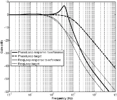
The round-trip (command to measured value) closed-loop responses for the system, using the original hand-tuned parameters (Table 1) are shown in Fig. 6. The phase loop response represents the entire control system of Fig. 5, whereas the frequency loop response represents the inner frequency-control loop. The phase loop has a bandwidth of about 2 Hz. The OLTF (open loop transfer function) is not shown graphically, but the forecast gain margin is 15.5dB and the phase margin is 42°.
To improve the response, “lambda-tuning” was used [12]. Targets were set for the desired closed-loop command-to-measured-value responses of the frequency control loop, and then the phase control loop. The targets are defined such that the responses should ideally behave as first-order low-pass filter responses to command signals. Firstly, the CLTF for the frequency-control loop:
HL
F
as
H D C
HL H D C
F F
1 1
1 1
where a is the target first-order response time. Secondly, the response for the phase-control loop:
bs P R Q F HL H D C HL H D C C Q R Q F HL H D C HL H D C C Q F F P F F P 1 1 ' 1 1 1 1 ' 1 1 1 (2)
where b is the target first-order response time.
Assuming that (1) can be satisfied, then (2) can be simplified to:
bs
P R as C R as C P P 1 1 1 1 1 1 1 (3)(1) and (3) can be solved, yielding:
s a f fa a f s Hfd s Lfd d f H d f L H s L CF ) 1 2 2 2
1 2 (4)
and s b p pb b p s ap s p a s CP 1 1 1
0 2 (5)
Equations (4) and (5) define the parameters for the two controllers CF and CP. Notably these controllers are
unconventional PIDA controllers, combined with low-pass filter elements. The acceleration terms (in s2) dramatically aid the stability, since they counter the phase lags. However, the risk in a practical system is that they (and indeed even the differential controls) introduce large amounts of noise due to the differentiation stages. It is only possible to use these terms, even with reduced magnitude, due to the good noise reduction of the measurement algorithms [13]
Setting the actual controls in practice involved the following steps, recognising that Fig. 5 is only an estimation of the actual system, and that the simple targets (1) and (2) do not fully define the response required in all scenarios:
evaluating (4), (5) and then examining OLTF (stability), CLTF (command-to-output) and response (command-to-measured-value) plots using MATLAB®
Trials of the chosen settings in the hardware implementation, making small changes to the settings of a and b
Reductions in the actual proportions of acceleration (s2) controls used, from those suggested in (4) and (5), to limit the response to measurement noise, as shown in table 1.
Increasing the amount of integral gain in CF to improve the initial settling to a new frequency, as shown in
table 1.
Repetition of trials of steps 2-4, in a range of scenarios, until the best behaviour is achieved.
The final set of control parameters are shown below in Table 1, together with the original hand-tuned values.
The resulting bode plots of the OLTF and the command-to-output CLTF are shown in Fig. 7 and Fig. 8. Forecast gain margin is 9dB and phase margin is 32°. Indeed, the hardware system is fast responding and on the limit of stability with this configuration. It is certainly found that if the Ka acceleration terms (in s2) are set to zero, the hardware is unstable. Conversely, if the Ka terms are increased to their theoretical values, noise becomes intolerable at the torque command output due to the increased CLTF response at high frequencies. The resulting responses (commands to measured values) are shown in Fig. 9. The phase loop bandwidth is increased from about 2 Hz to about 6Hz. Fig. 9 also shows the predicted deviations from the target “lambda-tuned” response, caused mainly by the ¼ reductions in the Ka gains to limit the effects of noise. The 10x boost to the integral gain of
CF causes almost no visible change to the responses shown on this figure.
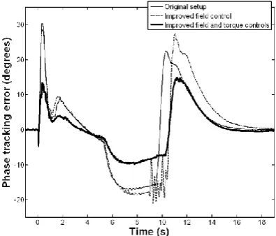
Using the improved controls, the HIL environment is now able to track the “pure simulation” case much more accurately. Fig. 10 shows the frequency profile, with the HIL results now tracking the simulation results much more closely than before (Fig. 10 to Fig. 13). The use of the lambda-tuning approach and the redesign of the torque control allows the peak phase tracking error to be reduced from 30° to 15°.
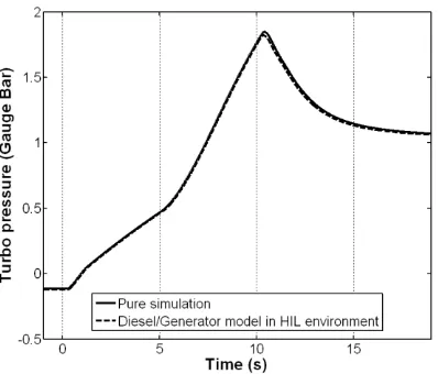
gauge bar) can be extracted from the HIL model in real time, and is shown in Fig. 14. This shows excellent agreement between the “pure simulation” and the HIL results.
4.3 Summary of incremental improvements
The incremental improvements in the fidelity of the hardware-in-the-loop environment, from the starting point of the basic controls used in [7], are summarised in Table 2. The incremental improvements are first the more powerful and faster-acting field control (section 4.1), followed by the improved phase tracking using lambda-tuning (section 4.2). The improvements in fidelity are also shown in Fig. 10 to Fig. 13.
5 Conclusions
A nested pair of PIDA (proportional-integral-derivative-acceleration) controllers have been tuned using “lambda-tuning”. These can be used to tightly match the phase of a large synchronous machine to the phase of a simulated machine. This allows a simulation of a multi-megawatt diesel engine to be interfaced with physical hardware to create a hardware in the loop (HIL) simulation environment, suitable for use with marine power system scenarios. The PIDA controllers allow the physical generator to track the phase of the simulated prime-mover to within 10-15° for scenarios with rates of change of frequency up to 5 Hz/s. The phase tracking is much better than this figure for less dynamic scenarios. The phase tracking accuracy cannot be significantly improved from the present performance, due to the physical limitations of the drive system and machine inertia. However, some further marginal improvements might be made by reducing the measurement algorithm times (Fig. 5). Care would be needed, however, since noise output from these algorithms will degrade the control signals, which make use of unconventional control terms in s2 to increase the control gain without becoming unstable.
For use within a HIL environment, it is also important that the field control for the synchronous generator be able to rapidly increase or decrease the field current, to track the simulation. This requires a field drive with sufficiently large voltage drive capability. Improved performance was shown in this paper by using a more capable field drive. A bidirectional field drive would also allow scenarios such as sharp voltage dips to be modelled.
Acknowledgements
The authors would like to acknowledge the funding and support provided by Rolls-Royce plc, which enabled this work to be undertaken.
References
[1] Butcher, M.S., Mattick, D., and Cheong, W.J.: 'Informing the AC versus DC debate - the Electric Ship Technology Demonstrator'. All Electric Ship (AES) Versailles, France, 2005
[2] Armstrong, M., Atkinson, D.J., Jack, A.G., and Turner, S.: 'Power system emulation using a real time, 145 kW, virtual power system'. European Conference on Power Electronics and Applications, 2005
[3] Langston, J., Suryanarayanan, S., Steurer, M., Andrus, M., Woodruff, S., and Ribeiro, P.F.: 'Experiences with the simulation of a notional all-electric ship integrated power system on a large-scale high-speed electromagnetic transient simulator'. Power Engineering Society General Meeting, 18-22 June 2006
[4] Liu, Y., Steurer, M., and Ribeiro, P.: 'A novel approach to power quality assessment: Real time hardware-in-the-loop test bed', IEEE Transactions on Power Delivery, 2005, 20, (2), pp. 1200-1201
[5] Qian, L., Liu, L., and Cartes, D.A.: 'A Reconfigurable and Flexible Experimental Footprint for Control Validation in Power Electronics and Power Systems Research'. Power Electronics Specialists Conference (PESC) Orlando, USA, 2007
[6] Woodruff, S., Boenig, H., Bogdan, F., Fikse, T., Petersen, L., Sloderbeck, M., Snitchler, G., and Steurer, M.: 'Testing a 5 MW high-temperature superconducting propulsion motor'. Electric Ship Technologies Symposium, 25-27 July 2005, pp. 206-213
[7] Roscoe, A.J., Mackay, A., Burt, G.M., and McDonald, J.R.: 'Architecture of a network-in-the-loop environment for characterizing AC power system behavior', IEEE Transactions on Industrial Electronics, 2010, 57, (4), pp. 1245-1253
[8] Hill, J.E., Kinson, A.S., Eraut, N.D., French, C., and Tumilty, R.M.: 'Motor Load Train Calculations for a Land Based Demonstrator for Marine Electrical Networks (DMEN)'. IEE International Conference on Power Electronics, Machines and Drives (PEMD), Edinburgh, UK, 2004
[9] Kao, M.H., and Moskwa, J.J.: 'Turbocharged Diesel-Engine Modeling for Nonlinear Engine Control and State Estimation', Journal of Dynamic Systems Measurement and Control-Transactions of the Asme, 1995,
117, (1), pp. 20-30
[10] Cooper., A.R., Morrow, D.J., and Chambers, K.D.R.: 'A Turbocharged Diesel Generator Set Model'. Universities’ Power Engineering Conference (UPEC) Glasgow, UK, 2009
[11] Kristiansson, B., and Lennartson, B.: 'Robust tuning of PI and PID controllers - Using derivative action despite sensor noise', IEEE Control Systems Magazine, 2006, 26, (1), pp. 55-69
[12] Lennartson, B., and Kristiansson, B.: 'Evaluation and tuning of robust PID controllers', IET Control Theory and Applications, 2009, 3, (3), pp. 294-302
Fig. 1 Generator torque due to 0.5pu load steps in four different modes
Fig. 2 Generator frequency due to 0.5pu load steps in four different modes
Fig. 3 Hardware-in-the-loop (HIL) environment for the diesel/generator model
80 kVA motor-generator
Fixed load
~
Local closed-loop control to force shared node voltages
Shared node
IG VN
IN
Key
Physical 3-phase cable connections Control signals/data
Measurements of voltages or currents Simulation boundary
Diesel-generator model calculates generator speed (frequency), due to electrical power output (IN, VN) and
governor action.
Real-Time Simulator & Controller
Integrate frequency to a target phase, and thus create a three-phase voltage set VN*
Control 80kVA genset to lock phase and magnitude of the actual VN triplet to the simulated VN*
Laboratory power hardware
network
M
Nomenclature
IG Vector of 3-phasecurrents from 80kVA generator
IN Vector of 3-phasecurrents flowing into hardware
VN Vector of 3-phase voltages at shared node in hardware
[image:12.595.58.530.549.707.2]Fig. 4 Generator frequency : Pure simulation and HIL using original setup
Fig. 5 Torque control system
Zero, or synthesised noise
Friction factor L = 0.093 nom
F
360 1
C
P(s)
Q(s)
Phase error (°)pu revolutions error, times Fnom
+
+
-C
F(s)
D(s)
1ds 1
H(s)
Hs 2 1L(s)
+ -LF(s)
1fs 1 Measured pu frequency
Q’(s)
nom F 360R(s)
s 1P(s)
1ps1 Measured Phase (°) Actual Phase (°) Actual frequency
+
-Target pu frequency
pu torque command
Phase change per second (°/s)
pu frequency error + + Feedforward throttle Drive response d = 0.03 H = 1.20
Phase measurement response 1.5 cycles averaging
p = 0.019
Frequency measurement
response 9 cycles averaging
f = 0.11 Zero, or
synthesised noise
Friction factor L = 0.093 nom
F
360 1
C
P(s)
Q(s)
Phase error (°)pu revolutions error, times Fnom
+
+
-C
F(s)
D(s)
1ds 1
H(s)
Hs 2 1L(s)
+ -LF(s)
1fs 1 Measured pu frequency
Q’(s)
nom F 360R(s)
s 1P(s)
1ps1 Measured Phase (°) Actual Phase (°) Actual frequency
+
-Target pu frequency
pu torque command
Phase change per second (°/s)
pu frequency error + + Feedforward throttle Drive response d = 0.03 H = 1.20
Phase measurement response 1.5 cycles averaging
p = 0.019
Frequency measurement
response 9 cycles averaging
f = 0.11
Fnom = 50 Hz
[image:13.595.116.489.324.544.2]Fig. 6 Command to measured-value response of the phase loop and frequency loop: hand-tuned parameters
Description Parameter Adjustments to (4) & (5) Final Value Original setup (Hand-tuned)
Target frequency CLTF response time a 0.15 sec
Target phase CLTF response time b 0.02 sec
Frequency loop CF Ki Boosted by 10x 3.432 2
“ Kp 8.935 8
“ Kd 1.352 1
“ Ka Reduced to ¼x 0.008589
Frequency loop CF low-pass filter cutoff
a
f
fa
66.6 ms
2.39 Hz 50 Hz (on Kd control only) 3.18 ms
Phase loop CP Ki 0
“ Kp 22.29 360x0.04 = 14.4
“ Kd 3.898
“ Ka Reduced to ¼x 0.02078
Phase loop CP low-pass filter cutoff
b
p
pb
11.1 ms 14.3 Hz [image:14.595.58.538.309.546.2]Fig. 7 OLTF and CLTF bode plots (Gain) for lambda-tuned torque control
Fig. 8 OLTF and CLTF bode plots (Phase) for lambda-tuned torque control
[image:15.595.198.393.540.707.2]Fig. 10 Generator frequency : Pure simulation and HIL using improved field and torque controls
Fig. 11 Voltage tracking for 0.5pu constant-power step HIL experiments
[image:16.595.194.392.525.694.2]Fig. 13 Power flow for 0.5pu constant-power step HIL experiments
Fig. 14 Turbo pressure
Description Original setup as per [7] tracking (80kVA field Improved voltage control)
Improved voltage tracking and DC
motor control
Maximum voltage
tracking error (pu) 0.058 0.024 0.020
Maximum
frequency-tracking error (Hz) 3.4 Hz 0.6 Hz 0.6 Hz
Maximum phase tracking error
(degrees) 30° 29° 15°
Maximum power flow
tracking error (pu) 0.055 0.022 0.018
[image:17.595.104.493.530.674.2]