City, University of London Institutional Repository
Citation
:
Renshaw, A. E. and Haberman, S. (2007). On simulation-based approaches to
risk measurement in mortality with specific reference to Poisson Lee-Carter modelling
(Actuarial Research Paper No. 181). London, UK: Faculty of Actuarial Science & Insurance,
City University London.
This is the unspecified version of the paper.
This version of the publication may differ from the final published
version.
Permanent repository link:
http://openaccess.city.ac.uk/2313/
Link to published version
:
Actuarial Research Paper No. 181
Copyright and reuse:
City Research Online aims to make research
outputs of City, University of London available to a wider audience.
Copyright and Moral Rights remain with the author(s) and/or copyright
holders. URLs from City Research Online may be freely distributed and
linked to.
Cass means business
Faculty of Actuarial
Science
and
Insurance
On Simulation-based
Approaches to Risk
Measurement in Mortality with
Specific Reference to Poisson
Lee-Carter Modelling.
Arthur Renshaw and
Steven Haberman.
Actuarial Research Paper
No. 181
May 2007
ISBN 978-1-905752-10-2
Cass Business School
106
Bunhill
Row
London
EC1Y
8TZ
On simulation-based approaches to risk measurement in mortality with specific
reference to Poisson Lee-Carter modelling.
A.E. Renshaw, S. Haberman
Cass Business School, City University, London, EC1Y 8TZ, UK
Abstract
This paper provides a comparative study of simulation strategies for assessing risk in mortality
rate predictions and associated estimates of life expectancy and annuity values in both period and
cohort frameworks.
Keywords:
Poisson modelling; Over-dispersion; Joint modelling; Negative binomial modelling;
Mortality projections; Mortality statistics; Simulated risk
1. Introduction
The trend in many countries to reform public sector pension provision and
encourage more private sector provision plus the widespread shift within private
sector pension provision towards more defined contribution schemes at the expense of
defined benefit schemes both mean, that, in the future, we can expect an increased
demand for post retirement annuity-type products.
From the viewpoint of insurance companies (and other providers) selling
annuity polices involves risk because of their exposure to uncertain future interest
rates and mortality rates. In this paper, we consider the second source of risk and the
need for effective risk measurement (and risk management) techniques.
Simulation techniques have been suggested in the literature as a means of
measuring risk, when modelling dynamic mortality rates and their impact on future
predictions of life expectancy and annuity values, because of the general intractability
of applying theoretical methods. We give further consideration to three such
simulation strategies (denoted A, B, C) which have been applied recently to Poisson
Lee-Carter (bilinear) modelling and extrapolation. Strategy A (semi parametric
bootstrap) is suggested in Brouhns
et al.
(2002) and illustrated (and compared with
Strategy B) in Brouhns
et al.
(2005). Strategy B (parametric Monte-Carlo) is
described and illustrated in Brouhns
et al.
(2002). Strategy C (residual bootstrap) is a
variant on the method described and illustrated in Koissi
et al.
(2006).
variable (Renshaw and Haberman (2003a & c)) and investigate the implications for
risk measurement. Additional consideration is given to aspects of parametric
simulation Strategy B in Section 6, to the impact of extra provision for variable
dispersion through joint modelling on simulation Strategies A and C in Section 7, and
to the impact of switching to negative binomial modelling on simulation Strategies A
and C in Section 8. A comparative assessment is made with a non-simulation method
of assessing risk in life expectancy predictions (Denuit 2006) in Section 9. Section 10
provides a discussion of the results and presents some concluding comments.
We conventionally refer to interval estimates as confidence intervals (CIs),
unless extrapolation is involved in their construction, as with statistics computed by
fixed cohort (Sections 5 to 9), when we refer to prediction limits.
2. Single parameter model
We illustrate the methodology in this section by considering a single
parameter model in the context of a well-known data set. In an investigation to test
whether the impact points of flying-bombs during World War II tended to be grouped
in clusters, Clarke (1946) divides an area of 144 sq. km. in south London into
n
= 576
squares of ¼ sq. km., and makes a count of the number of impact points in each
square. The (grouped) results are as summarised in the first two rows below:
Number of impacts per square
d
i
0
1
2
3
4
7
Number of squares or frequency
f
i
229
211
93
35
7
1
Predicted number of squares
f
ˆ
i
227
211
99
31
7
2
Deviance residual
r
i
-1.3655 0.0693 0.9579 1.6962 2.3486 4.0111
Modelling the number of impacts
D
i
per square
i
(= 1, 2,…,
n
) as independent
identically distributed Poisson random variables
D
i
~
Poi
(
e
i
µ
)
, with an assumed
single unit of exposure to the risk of impact, the same for all squares
(
e
i
=
1
∀
i
)
,
gives
9323
.
0
ˆ
=
=
=
µ
d
d
n
i
i
.
The frequency distribution predicted by the fitted model and recorded (to the nearest
whole number) in the third row of the above table, is indicative of a good fit.
The associated (classical) inference is standard. Thus,
µ
is estimated by
maximising the log likelihood
(
log
)
const
.
log
=
µ
−
µ
+
i
i
i
e
d
L
n
L
µ
=
µ
∂
∂
−
−
µ
=
µ
ˆ
log
E
1
ˆ
2
2
, and large sample CI
n
z
µ
±
µ
ˆ
1
−
α′
/
2
ˆ
where
z
1
−
α′
/
2
is the usual standard normal deviate.
Under the alternative canonical parameterisation (log link)
log
µ
=
α
, which
forms the basis of more complex parameterised structures and the second of the
simulation strategies considered below. Hence,
α
ˆ
=
log
d
with variance
α
=
α
∂
∂
−
−
α
=
α
exp
ˆ
1
log
E
1
ˆ
2
2
n
L
which is the inverse
−
1
of the information matrix .
We focus on the construction of CIs for
µ
by simulation and consider three
possible strategies. At each simulation
j
(= 1, 2, …,
N
)
A: simulate responses
d
i
(
j
)
∀
i
by sampling
Poi
(
d
ˆ
i
)
and compute
µ
(
j
)
by fitting
(
j
)
~
Poi
(
(
j
)
)
i
D
µ
.
B: randomly generate a standard normal deviate
ε
(
j
)
~
N
(
0
,
1
)
to simulate the parameter as
(
)
.
(
)
ˆ
log
1
ˆ
j
j
n
α
ε
φ
+
α
=
α
and compute
µ
(
j
)
=
exp
α
(
j
)
. Here,
φ
is the optional scale parameter.
C: simulate responses
d
i
(
j
)
∀
i
by sampling
{
d
i
}
with replacement
and compute
µ
(
j
)
by fitting
(
j
)
~
Poi
(
(
j
)
)
i
D
µ
.
After
N
= 5,000 (say) such simulations using each strategy in turn, compute the
N
N
and
(
1
)
100
100
2
2
α′
α′
−
order statistics of
{
µ
(
j
)
}
to give a two-sided
(
1
−
α′
)
100
%
CI for
µ
, together with the median
µ
~ to compare with
µ
ˆ .
For comparison purposes, we record both the theoretical based 95% CI for
µ
,
together with the simulated 95% CIs and median based on 5,000 simulations, under
each strategy in the table below and note the exceptionally close agreement between
corresponding figures.
m.l.e.
95% C.I.
Simulation
Strategy
A
Simulation
Strategy
B
Simulation
Strategy
C
9323
.
0
ˆ
=
µ
(0.853, 1.011)
9323
.
0
~
=
µ
(0.856, 1.012)
9325
.
0
~
=
µ
(0.857, 1.016)
9323
.
0
~
=
µ
(0.854, 1.016)
Here, under simulation Strategy A,
d
ˆ
i
=
µ
ˆ
, while as a consequence of the final
fitting stage in Strategies A and C,
d
n
i
j
i
j
=
Under Strategy B, the parameter
α
is simulated on scaling the standard
normal deviate by the standard error of
α
ˆ , before centring on
α
ˆ . In addition it is
possible to allow for dispersion in the data under this strategy through the
incorporation of an optional scale parameter
φ
(>0). The theoretical justification for
including
φ
is given in Section 5. For the Poisson distribution (without dispersion),
we set
φ
=
1
.
Strategy C is the basic bootstrap for targeting the mean, described in Chapter 2
of Efron and Tibshirani (1993): subject to a different (but equivalent) treatment of the
simulated
{
µ
(
j
)
}
, using order statistics. It is necessary in this paper for us to take a
different perspective of this strategy by sampling residuals, in order to be able to
manage more general parametric structures. We follow Chapter 9 (and Section 9.4 in
particular) of Efron and Tibshirani (1993) on bootstrapping residuals in regression
models, making the necessary changes to the subsequent mapping of bootstrap
residuals into bootstrap responses. These changes are needed in order to match with
the Poisson error assumption, as opposed to the additive error structure, implied by
equation (9.26) of Efron and Tibshirani (1993). Then the residual bootstrap version
of Strategy C reads as follow:
C: simulate residuals
r
i
(
j
)
∀
i
by sampling }
{
r
i
with replacement, then
map the bootstrap residuals to responses
r
i
(
j
)
d
i
(
j
)
∀
i
and compute
µ
(
j
)
by fitting
(
j
)
~
Poi
(
(
j
)
)
i
D
µ
.
Bootstrap deviance residuals are mapped by solving the relationship
(
)
(
i
i
)
i
i
i
i
i
i
d
d
d
d
d
d
d
r
ˆ
ˆ
log
2
ˆ
sign
−
−
−
=
(1)
for
d
i
when
)
(
j
i
i
r
r
=
. Therefore, suppressing the suffix
i
for clarity of notation, and
using the prefix * (instead of
j
) to denote bootstrap values, this implies that we require
the appropriate root
d
*
of
(
1
ˆ
)
ˆ
,
0
log
)
(
g
d
=
d
d
-
d
+
a
−
c
*
d
≥
(2)
where
a
d
c
*
r
d
ˆ
2
ˆ
,
ˆ
log
ˆ
2
*
−
=
=
, when mapping
*
*
d
r
. The derivatives of g
0
0
1
)
(
,
ˆ
log
)
(
g
′
=
−
′′
=
>
∀
d
>
d
d
g
a
d
d
imply that
d
=
d
ˆ
is a minimum and that the graph of g(
d
) vs.
d
(
d
>0) is concave.
There are either one or two roots in this range. The required root is determined by the
sign of the residual
*
r
and lies to the right of the minimum (
d
>
d
ˆ
) when
r
*
> 0, and
to the left of the minimum (
d
<
d
ˆ
) when
r
*
< 0. The root is readily determined by
within the limits of the domain
{
d
:
d
≥
0
}
. Note the two special cases
r
*
<
0
,
c
ˆ
*
>
0
and
r
*
=
−
2
d
ˆ
,
c
ˆ
*
=
0
, each of which implies
d
*
=
0
is the required root.
The process is illustrated in Fig.1, with each frame corresponding to a
different entry in the tabulated data above. Restoring the suffix
i
, the bootstrap
residual mapping,
*
i
*
i
d
r
, takes the special form
r
i
*
d
i
, which involves the
mapping of bootstrap residuals to matching observations as a consequence of the
simplicity of the model structure based on a single location parameter
µ
.
3. A two parameter model (Gompertz s law)
In order to take the development further, we take a well-known data set from
the mortality literature and apply a model, which can be presented in a linear form. In
a study to graduate the UK pensioners’ widows’ 1979-82 mortality experience Forfar
et al.
(1988) apply Gompertz’s law. A short extract of the raw data
(
d
x
,
e
x
)
comprising the respective number of deaths and matching exposures to the risk of
death at age
x
, together with the graduated force of mortality
µ
ˆ , the expected number
x
of deaths
d
ˆ predicted by the model, in addition to the deviance residuals
x
r
x
, is
recorded below:
x
e
x
µ
ˆ
x
d
x
d
ˆ
x
r
x
20
4.0 .00038219
0
0.00 -0.0553
30
36.0 .00090617
0
0.03 -0.2554
40
115.5 .00214854
0
0.25 -0.7045
50
378.5 .00509423
3
1.93 0.7132
60 1029.0 .01207848
14 12.43 0.4368
70
941.0 .02863823
21 26.95 -1.1925
80
323.5 .06790162
25 21.97 0.6332
90
30.5 .16099560
6
4.91 0.4750
100
1.0 .38172269
0
0.38 -0.8738
The complete table (Forfar
et al.
(1988) Table 15.5 (& 15.1)) is given by individual
year of age from 17 to 108, and we note that the bulk of the exposure lies in the age
range 45 to 90.
Graduation proceeds by modelling the number of deaths as independent
Poisson responses
D
x
~
Poi
(
e
x
µ
x
)
where
log
µ
x
=
α
+
β
x
(which is a
re-parameterisation of Gompertz’s law
x
x
=
Bc
µ
). The parameters
θθθθ
=
(
α
,
β
)
T
are
estimated first using numerical methods in order to maximise the log likelihood
(
log
)
const
log
=
ω
µ
x
−
µ
+
x
x
x
x
x
d
e
L
(3)
followed by the computation of
x
x
x
x
=
α
+
β
x
d
=
e
µ
Zero/one weights
ω
x
are included in the formulation so that we can deal with
empty/non-empty data cells. The variance-covariance matrix of the parameter
estimates is the inverse
−
1
of the information matrix
=
ω
ω
ω
ω
x
x
x
x
x
x
x
x
x
x
x
x
d
x
d
x
d
x
d
ˆ
ˆ
ˆ
ˆ
2
,
comprising the (expectations of the) second order partial derivatives of
−
log
L
with
respect to the two parameters.
We focus on the simulation of CIs for the age-specific force of mortality
µ
x
,
life expectancy
e
(
x
)
and level immediate annuity
a
(
x
)
with given discount factor
v
(and fixed rate interest), where
x
i
i
i
x
x
i
i
x
i
x
l
v
l
x
a
l
q
l
x
e
≥
+
≥
+
+
=
−
=
0
2
1
1
)
(
ˆ
,
)
ˆ
1
(
)
(
ˆ
and
x
x
x
x
x
l
q
l
q
ˆ
≈
1
−
exp(
−
µ
ˆ
),
+
1
=
(
1
−
ˆ
)
.
We use the same three simulation strategies, which are generalised to read as follows:
At each simulation
j
A: simulate responses
(
j
)
x
d
by sampling
Poi
(
d
ˆ
x
),
∀
x
=
x
1
,
x
2
,...,
x
n
,
then compute
(
j
)
x
µ
by fitting
(
)
~
Poi
(
(
j
)
)
x
x
j
x
e
D
µ
∀
x
before computing the statistics of interest.
B: randomly generate a pair of N(0,1) deviates
εεεε
(
j
)
(
)
T
2
)
(
1
,
)
(
ε
j
ε
j
=
to simulate parameters according to
θθθθ
(
j
)
= θθθθ
ˆ
+
φ
εεεε
(
j
)
where is the Cholesky factorisation (‘square root’) matrix of the
variance-covariance matrix
−
1
,
φ
is the optional scale parameter
before computing
(
j
)
x
µ
(here
µ
(
x
j
)
=
exp(
α
(
j
)
+
β
(
j
)
x
)
∀
x
)
and the statistics of interest.
C: simulate residuals
r
x
(
j
)
∀
x
by sampling
{
r
x
}
with replacement,
map the bootstrap residuals to responses
r
d
j
x
x
j
x
∀
)
(
)
(
then compute
(
j
)
x
µ
by fitting
(
)
~
Poi
(
(
j
)
)
x
x
j
x
e
D
µ
before computing the statistics of interest.
Subject to centring
x
at age 70 and scaling (dividing) by 50, the parameter
3166
.
4
ˆ
,
5530
.
3
ˆ
=
−
β
=
α
−
−
=
−
038653
.
0
001907
.
0
001907
.
0
001539
.
0
1
,
−
=
19050
.
0
04862
.
0
0
03923
.
0
.
The simulated median and two-sided 95% (percentile based) CIs for the force of
mortality, life expectancy and 4% fixed rate annuity at ages (
x
= 45, 65, 75), using all
three strategies (with
N
= 5,000) are depicted in Fig 2. In addition, the age-specific
force of mortality, life expectancy and annuity value based on model estimates
(m.l.e.) are also depicted for comparison. Here, the 95% CI for the force of mortality
is based on the close approximation
)}
ˆ
(
E
2
exp{
)
ˆ
(
Var
)
ˆ
(
Var
µ
x
≈
η
x
η
x
where
η
ˆ
x
=
α
ˆ
+
β
ˆ
x
,
and the 95% CIs for life expectancy and annuity values are based on the approximate
expressions for the respective variances
2
0
)
(
ˆ
ˆ
ˆ
)}
(
ˆ
{
Var
≈
+
+
≥
+
+
+
x
j
x
j
i
j
x
j
x
j
x
l
j
x
e
l
e
p
q
x
e
(4)
2
0
)
(
ˆ
ˆ
ˆ
)}
(
ˆ
{
Var
≈
+
+
≥
+
+
+
x
j
j
x
j
i
j
x
j
x
j
x
l
j
x
a
v
l
e
p
q
x
a
(5)
with initial exposures
x
x
i
x
e
d
e
≈
+
2
1
(e.g. Benjamin and Pollard (1980), Chapter 17).
We note the following:
1. The simulated histograms (not shown) underpinning the CIs are essentially
symmetric throughout. In addition, the upper and lower simulated percentiles
displayed are effectively the same as the 95% (two-sided) confidence limits
calculated using the simulated mean and variance.
2. Within each frame, the degree of vertical alignment of the central measures
(medians and maximum likelihood point estimate) indicates the extent of the
agreement between the respective first moment estimated targets. In this
respect, Strategies A and B are closely aligned with each other and with the
maximum likelihood estimate in all cases.
3. The reason for the inconsistent alignment under Strategy C is the presence of
bias in the residuals due to the paucity of exposure at ages (with zero deaths)
below age 45: this gives rise to a run of small negative residuals which is
unrepresentative of the randomly distributed residuals pertaining to the
remainder of the age range.
5. Frames depicting the force of mortality (1
st
column) are not drawn to the same
scale for practical reasons. Allowing for the relative magnitude of
µ
x
, the
coefficient of variation (relative error) is observed to decrease with increasing
age, on the basis of the following representative (Strategy A) values:
Age
45
65
75
Coefficient of variation
0.114 0.048 0.040
6. Frames depicting life expectancy (2
nd
column) and the fixed rate annuity using
a 4% interest rate (3
rd
column) are presented on the same respective scales and
may be compared column-wise. On this evidence, there is no obvious
emerging pattern in the interval widths with age.
Simulation Strategies A and C are conducted with due attention to the vector
of weights
ω
x
, ensuring that any empty data cells are preserved as such, at each stage
of the simulation process.
Under Strategy C, the mapping of bootstrap residuals
(
)
(
j
)
x
j
x
d
r
is as
described in Section 2 with
x
replacing the suffix
i
, resulting in
d
x
(
j
)
≠
d
x
in general.
We remark that this mapping is invariant to the scaling of residuals (by
φ
). Thus
simulation Strategy B would appear to be the only one of the three strategies
considered, which is sensitive to the inclusion of a scale parameter. In this example,
we again set
φ
=
1
, but we illustrate and discuss the effects of both estimating and
generalising
φ
as a function of age
x
, in later sections.
4. A four parameter non-linear model (Makeham s second law)
In this section, we illustrate the approach for a model, which is non-linear and
involves 4 parameters. In a study to graduate the UK male assured lives 1979-82
mortality experience (based on policy counts and policy duration 5+ years), Forfar
et
al.
(1988) apply the enhanced Makeham formula
)
exp(
0
1
1
0
x
x
x
=
α
+
α
+
β
+
β
µ
.
Using the same notation as Section 3, an extract of the data
(
d
x
,
e
x
)
adjusted before
modelling to allow for duplicated policies, together with the model estimates, are as
follows:
x
e
x
µ
ˆ
x
d
x
d
ˆ
x
r
x
The adjustment to the numbers of deaths and matching exposures by dividing both
quantities by the so-called variance ratios based on duplicated policy counts, is as
described in Forfar
et al.
(1988) and need not directly concern us here. The complete
table (Forfar
et al.
(1988) Table 17.9 with additional reference to Tables 17.6 & 17.8)
is given by individual year of age from 10 to 90. We note that there is a relative
scarcity of exposure below age 20.
The parameters
θθθθ
=
(
)
T
1
0
1
0
,
α
,
β
,
β
α
are estimated by maximising the Poisson
log likelihood (3) and
µ
ˆ
x
,
d
ˆ
x
and
r
x
computed subsequently. One possible method of
fitting through linearisation is by declaring a GLM with
Poisson responses
d
x
e
x
, expectation
µ
x
, weights
ω
x
=
e
x
, identity link
and conducting the iterative linear fitting routine:
Set the starter value
ρ
i
=
ρ
1
=
0
.
0005
(
say
)
↓
Estimate the parameters
(
α
0
,
α
1
,
β
,
γ
)
by fitting
x
x
x
i i
x
x
+
β
ρ
+
γ
ρ
α
+
α
=
µ
0
1
e
e
↓
Compute
ρ
i
+
1
=
ρ
i
+
γ
ˆ
β
ˆ
to update
ρ
i
↓
Stop when
{
ρ
i
}
converges
Here
ρ
is an auxiliary parameter (assumed known, so that the expression for
µ
x
is
linear in the other four parameters), while the iterative routine is based on a
linearisation method for fitting non-linear parameters in the covariates of a GLM
(Section 11.4, McCullagh and Nelder (1989); Section 6, Renshaw (1991)).
Convergence is rapid with
α
ˆ
0
,
α
ˆ
1
as given in the limit, and
β
ˆ
0
=
log
β
ˆ
,
β
ˆ
1
=
ρ
i
,
(
γ
ˆ
=
0
)
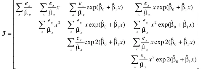
in the limit. Details of the symmetric information matrix are as follows:
β
+
β
µ
β
+
β
µ
β
+
β
µ
β
+
β
µ
β
+
β
µ
µ
β
+
β
µ
β
+
β
µ
µ
µ
=
)
ˆ
ˆ
(
2
exp
ˆ
)
ˆ
ˆ
(
2
exp
ˆ
)
ˆ
ˆ
(
2
exp
ˆ
)
ˆ
ˆ
exp(
ˆ
)
ˆ
ˆ
exp(
ˆ
ˆ
)
ˆ
ˆ
exp(
ˆ
)
ˆ
ˆ
exp(
ˆ
ˆ
ˆ
1
0
2
1
0
1
0
1
0
2
1
0
2
1
0
1
0
x
x
e
x
x
e
x
e
x
x
e
x
x
e
x
e
x
x
e
x
e
x
e
e
x
x
x
x
x
x
x
x
x
x
x
x
x
x
x
x
x
x
x
x
x
x
x
x
x
x
x
x
x
x
Subject to the same centring and scaling of
x
(Section 3), the parameter estimates and
Cholesky factorisation of the variance-covariance matrix
−
1
are as follows:
595709
.
4
ˆ
,
329023
.
3
ˆ
,
004319
.
0
ˆ
,
003788
.
0
ˆ
0=
−
α
1=
−
β
0=
−
β
1=
[image:12.595.143.484.566.687.2]=
−
−
−
00844291
.
0
00927452
.
0
01309409
.
0
03829598
.
0
0
00476708
.
0
00106814
.
0
00708817
.
0
0
0
00002625
.
0
00024399
.
0
0
0
0
00022455
.
0
The equivalent simulations (Section 3), depicting the median and 95% (percentile)
CIs for the force of mortality, life expectancy and 4% fixed rate annuity (x = 45, 65,
75), using all three strategies, plus maximum likelihood estimates, (including CIs for
life expectancy and annuities using (4) and (5)), are presented in Fig 3. We note the
following:
1. As in Section 3, we have not shown any of the simulated histograms, which
are symmetrical throughout: a feature reflected in the symmetry of the CIs.
2. Within each frame, the close vertical alignment (including that under Strategy
C), of the central measures (medians and maximum likelihood estimate).
3. Within each frame, prediction intervals under Strategies A and B are
essentially the same, and marginally narrower than those under Strategy C.
The m.l.e. CIs are marginally wider still, in general.
4. The comparative narrowness of the CIs compared with their counterparts in
the UK pensioners widow study (Fig 2). This is further reflected in a typical
comparison of the coefficient of variation for
µ
x
under the respective studies:
Age
45
65
75
Male assured lives
0.0092 0.0052 0.0069
Pensioners widows
0.114
0.048
0.040
Force of mortality: coefficient of variation (Strategy A)
5. As before, frames depicting life expectancy (2
nd
column) and the 4% fixed rate
annuity (3
rd
column) are presented on the same respective scales and can be
compared column-wise, with no evidence of an emerging age pattern in the
interval widths.
5. Multiple parameter non-linear age-period models
This study features the UK male pensioner 1983-2003 mortality experience
illustrated in Fig 4. Here we have plotted the log crude mortality rates (continuous
profiles) against period
t
=
t
1
,
t
2
,...,
t
n
for selected ages in the range
x
=
x
1
,
x
2
,...,
x
k
,
using data
(
d
xt
,
e
xt
)
comprising the respective number of deaths and matching
exposures to the risk of death at age x in calendar year t. Ages range from 51 to 104
with roughly 95% of the total exposure in the age range 62-89 and 95% of the total
deaths in the range 66-93. The rectangular data set is an updated version, with
expanded age range, of the UK male pensioner 1983-94 experience modelled
previously (Renshaw and Haberman (2003b)). We note that about 5% of the data
cells are empty.
The numbers of deaths are modelled as independent Poisson responses
)
(
Poi
~
xt
xt
xt
e
0
,
1
;
log
:
LC
µ
=
α
+
β
κ
β
=
κ
=
n
t
x
x
t
x
x
xt
,
(6)
.
1
,
0
);
(
)
(
log
:
LP
µ
=
α
+
β
−
+
γ
−
γ
1=
γ
=
β
=
x
x
t
t
n
t
n
x
x
xt
t
t
t
t
n
(7)
The non-linear (LC) structure is that generally attributed to Lee and Carter (1992)
(subject to a change in their usual parameter constraints: see Section 6), while the
linear Poisson (LP) structure has been suggested and used previously in a similar
context by Renshaw and Haberman (2003a). The structures are characterised by
writing
1
)
,
(
F
);
,
(
F
)
exp(
α
=
=
µ
xt
x
x
t
x
t
n
.
(8)
In the spirit of historical CMI Bureau practice (e.g. CMI (1999)), we interpret (8) as
the product of a static life-table
exp(
α
x
)
summarising the over-all main age effects
with regard to the calendar year
t
n
, and a mortality reduction factor
F
encapsulating
age-specific dynamic adjustments.
The structures are fitted by maximising the log likelihood expression (3) in
which
x
is replaced by
x,t
(or minimising the current model deviance
−
2
log
(
L
L
f
)
where
L
f
is the likelihood of the full or saturated model: characterised by equating
the fitted and actual numbers of deaths). We use an iterative method described in
Renshaw and Haberman (2006) when fitting LC and the software package GLIM
(Francis
et al.
(1993)) when fitting LP. The model fitting of LC is discussed further
in Section 6. For LP model fitting, the constraints
γ
1=
γ
=
0
n
t
t
apply and the
resulting
β
ˆ are scaled (together with the compensating scaling of the multiplicative
x
terms
(
t
n
−
t
)
), to comply with the auxiliary constraint
β
=
1
x
x
. This approach to
LP model fitting, in which both components of
µ
xt
(equation (8)) are fitted
simultaneously, differs from the two-stage model fitting approach discussed in
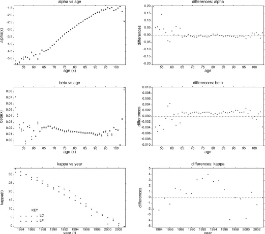
Renshaw and Haberman (2003a). The fitted log mortality rates
log
µ
ˆ
xt
under both
structures have been superimposed in Fig 4. The underpinning parametric structures
are depicted in Fig 5, in which we have superimposed the respective parameter
estimates under both structures (LH frames) and plotted their differences in the
matching RH frames: the imposition of equivalent parameter constraints under LC
and LP modelling provides the basis for parameter comparisons. (We refer loosely to
t
t
n
t
=
−
κ
under LP modelling as parameters here).
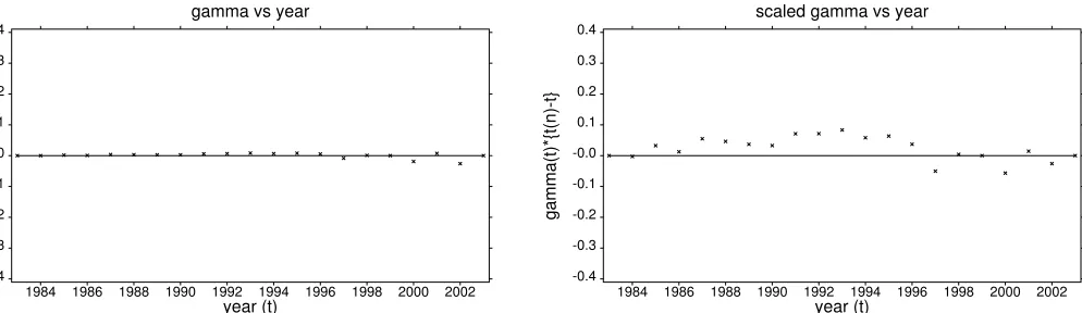
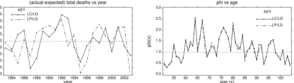
The extra term involving
γ
t
under LP modelling ensures that the annual actual
and expected total deaths are the same, (in addition to improving the quality of the
fit). The estimates of
γ
t
and
γ
t
(
t
n
−
t
)
are depicted in Fig 6a, together with the
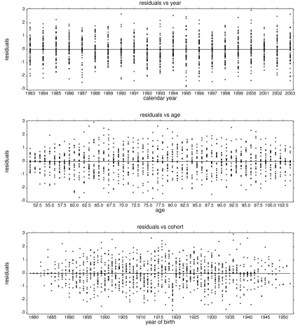
compared with the original Gaussian formulation, while pattern-free differences are
indicative of a good fit. The small reported deviations from zero under LP modelling
(RH frame Fig 6b) are directly attributable to the paucity of exposure at ages 103 and
particularly 104. Residual plots under LC modelling are similar to those under LP
modelling (Fig 7) and hence, have not been presented. Both sets of residual plots are
therefore supportive of the respective model structures. In particular, the residual plot
against year of birth, together with further diagnostic plots designed to detect residual
cohort effects (not shown), fail to identify any obvious residual systematic cohort
effect.
Mortality rates are extrapolated according to
0
),
,
(
F
)
ˆ
exp(
s
=
α
+
>
µ
x,
t
+
x
x
t
n
s
s
n
where
( )
ˆ
ˆ
,
0
exp
)
,
(
F
:
LC
x
t
n
+
s
=
θ
β
x
s
s
>
;
θ
ˆ
=
−
κ
ˆ
t
1(
t
n
−
t
1
)
0
),
ˆ
exp(
)
,
(
F
:
LP
x
t
n
+
s
=
−
β
x
s
s
>
when forecasts are generated by applying a random walk with drift parameter
θ
to the
time series {
κ
ˆ } under LC modelling. (We note that, when the random walk with
t
drift is the preferred time series, selected here by testing for the best ARIMA model
for {
κ
ˆ }, forecasts are generated by extrapolating the straight line joining the two
t
extremes
(
t
1
,
κ
ˆ
t
1)
and
(
t
n
,
κ
ˆ
t
n)
of the time series, with
κ
ˆ
t
n=
0
). Thus, under this
special case, it is only necessary to resort to the use of a standard time series package
in order to establish the appropriateness of the random walk with drift: refitting the
time series to generate forecasts at each simulation is redundant. Under LP
modelling: referring to equation (7) and Fig 6a, we extrapolate
β
ˆ
x
(
t
n
−
t
)
while
setting the extrapolation of
γ
ˆ
t
(
t
n
−
t
)
to zero.
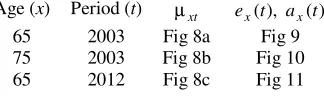
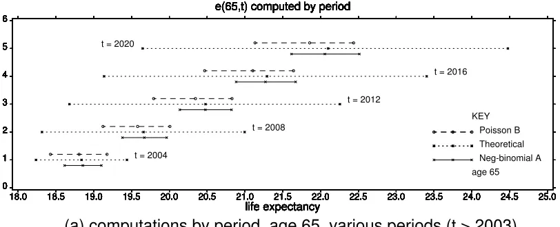
We investigate age-period specific life expectancies
e
x
(
t
)
and age-period
fixed rate annuities
a
x
(
t
)
with discount factor
v
, under both the cohort method of
computing:
)
(
)
(
)
(
ˆ
,
)
(
)}
(
ˆ
1
){
(
)
(
ˆ
0
2
1
1
t
l
v
i
t
l
t
a
t
l
i
t
q
i
t
l
t
e
x
i
i
i
x
x
x
i
i
x
i
x
x
≥
+
≥
+
+
+
=
+
−
+
=
(9)
where
)
(
)}
(
ˆ
1
{
)
1
(
),
ˆ
exp(
1
)
(
ˆ
t
l
1
t
q
t
l
t
q
x
≈
−
−
µ
xt
x
+
+
=
−
x
x
,
and the period method of computing, in which the variation in
t
in the above
expressions is suppressed, as in Section 3.
The simulation strategies are as described in Section 3, subject to the
required, involving the extrapolation of
j
x,
t
xt
∀
µ
(
)
with respect to
t
, prior to
computing the statistics of interest. For simulation Strategy B the parametric vector
basis
θθθθ
comprises 2
k
+
n
– 2 components
(
T
T
T
)
T
,
,
:
LC
θθθθ =
α
α
α
α
x
ββ
β
β
x
κ
κκ
κ
t
with
β
x
1=
1
,
κ
t
n=
0
(10)
(
T
T
T
)
T
,
,
:
LP
θθθθ =
α
α
α
α
x
β
ββ
β
x
γγγγ
t
with
γ
1=
0
,
γ
=
0
n
t
t
(11)
and the variance-covariance matrix is computed as the inverse of the information
matrix, (based in turn on the second order partial derivatives of
−
log
L
). Under LC
modelling, details of the information matrix are given in Appendix A. Under LP
modelling, since period effects are treated deterministically, the terms
κ
t
≡
t
n
−
t
do
not feature as explicit components of
θθθθ
, while the variance-covariance matrix is
readily available from standard linear regression packages, such as GLIM. Details of
the information matrix are given in Appendix B. It is then necessary to scale the
simulated
β
x
, (coupled with the compensating scaling of the multiplicative
κ
t
or
)
(
t
n
−
t
terms, as the case may be), in order to comply with the constraint
β
=
1
x
x
.
The justification for the introduction of dispersion into the Poisson modelling
assumption comes from the following:
( )
u
u
D
D
e
D
xt
xt
xt
xt
xt
xt
=
ω
φ
=
µ
=
,
Var
(
)
V
{
E
(
)}
;
V
)
(
E
(12)
with positive scale parameter
φ
(>1 for over-dispersion), zero-one prior weights
ω
xt
,
and the characteristic Poisson variance function V(
u
) =
u
. The fitted structure
minimises the model deviance
(
)
=
φ
ω
−
φ
−
=
xt
d
d
xt
xt
f
xt
xy