Multidimensional partitioning and
bi-partitioning: analysis and application to
gene expression datasets
Gabriela Kalna
∗J. Keith Vass
†Desmond J. Higham
‡November 7, 2006
Abstract
Eigenvectors and, more generally, singular vectors, have proved to be useful tools for data mining and dimension reduction. Spectral clus-tering and reordering algorithms have been designed and implemented in many disciplines, and they can be motivated from several different standpoints. Here we give a general, unified, derivation from an ap-plied linear algebra perspective. We use a variational approach that has the benefit of (a) naturally introducing an appropriate scaling, (b) allowing for a solution in any desired dimension, and (c) dealing with both the clustering and bi-clustering issues in the same framework. The motivation and analysis is then backed up with examples involv-ing two large data sets from modern, high-throughput, experimental cell biology. Here, the objects of interest are genes and tissue sam-ples, and the experimental data represents gene activity. We show that looking beyond the dominant, or Fiedler, direction reveals important information.
Keywords: data mining dimension reduction, feature selection, graph Laplacian, Fiedler vector, microarray, singular value decomposition, tumour classification.
∗Department of Mathematics, University of Strathclyde, Glasgow G1 1XH, UK. Sup-ported by EPSRC grant GR/S62383/01.
†The Beatson Institute for Cancer Research, Glasgow G61 1BD, UK
AMS Subject Classification: 65F15, 92C37.
1
Background
Modern technology is responsible for a data deluge that has driven the need for computational algorithms in data mining and dimension reduction. Many large scale data sets take the form of a matrix,W, withwijrepresenting some relationship between objects labeled i and j. If objects i and j come from the same list, then W will be square. For example, wij may be a correlation coefficient between stock prices [3]. If objects i and j come from different lists, thenW can be rectangular. For example,wijmay represent the number of occurrences of word i in document j, [7].
Given its fundamental role in applied matrix analysis, it is not surprising that the singular value decomposition is an extremely useful tool for summa-rizing important information from such data sets. We refer to [11] for a list of areas where the general concept of spectral clustering has been applied.
Data mining with singular vectors can be motivated from a number of different directions and is closely related to ideas in Principle Component Analysis [20, 21], support vector machines/kernel based methods [16], ma-chine learning [14] and multidimensional scaling [6]. Our main contribution here is to present a simple, unified framework that justifies the approach while automatically
(a) introducing an appropriate scaling,
(b) allowing for a solution in any desired dimension, and
(c) dealing with both the clustering and bi-clustering issues.
In particular, this work extends that in [11] to allow for bi-clustering of non-square data and for projecting to arbitrary dimension.
To illustrate the analysis, and in particular to emphasize that more than just the first, or Fiedler, direction can be important, we also present numer-ical results on microarray expression data sets.
Throughout this work we use the following notation:
• k · k2 denotes the Euclidean norm,
• 1 denotes the vector in RN with all elements equal to one.
• I denotes an identity matrix whose dimension is clear from the context,
• 0r×s denotes the zero matrix in Rr×s.
2
Square Symmetric Case
In this section, we consider the case where W = WT ∈ RN×N is a square, symmetric matrix with non-negative elements, wij ≥0, and with allwii= 0. Here, there are N objects of interest and wij = wji represents the pairwise similarity of objects iandj. We take the view that a large value ofwijmeans that objects i and j are very similar. (Some references use the opposite convention, taking a large wij to mean very dissimilar, but, of course, a simple transformation such as wij 7→ maxr,swrs −wij converts that format into ours.)
When N is large, the pairwise similarity data in W represents a vast amount of information. In order to create a manageable subset of informa-tion that can be easily visualized or otherwise processed, it is necessary to summarize the data. Three typical, and closely related, tasks are
1. re-order the objects so that objects close together have strong similarity and objects far apart have weak similarity [2, 10],
2. map each object to a point in a low dimensional space,Rs, so that objects close in Euclidean distance have strong similarity and objects far apart in Euclidean distance have weak similarity [4],
3. split the objects in to two or more clusters so that objects in the same cluster have strong similarity and objects in different clusters have weak similarity [9].
In this work we focus on task 2, while noting that a method for task 1 then follows automatically—map into R1 and use the resulting N numbers to order the objects. Similarly, having achieved 2, there are straightforward ways to produce a clustering for task 3 [1, 17].
Now, focusing on task 2, for some s < N our aim is to find vectors
{y[1], y[2], . . . , y[N]}with each y[j]∈
Rs such that the jth object is associated with the vectory[j]. The idea is that the relative distanceky[i]−y[j]k
the pairwise similarity weight, wij. We began with (N2−N)/2 real numbers (that is, the elements of W, allowing for symmetry and a zero diagonal) and we hope to reduce this to N s numbers (in the vectors {y[j]}N
j=1). Clearly, if
N is large and sN then this is a significant compression. Given thatky[i]−y[j]k
2 should be small when wij is large and vice versa, a reasonable starting point is to consider choosing {y[j]}N
j=1 to minimize
P
i
P
jky[i]−y[j]k22wij. However, since this objective function can gener-ally be decreased simply by rescaling y[k]7→y[k], we must incorporate some
normalizing constraint. Considering that the kth object gets mapped to a vector whose first component is y1[k], we will normalize the two-norm of the vector making up these components, when scaled by the square root of the corresponding degree; that is, set
√
d1y1[1]
√
d2y1[2]
.. . .. .
√
dNy1[N]
2
= 1.
Here dk := PNr=1wkr is the degree of object k, that is, the total weight associated with node k in the corresponding graph. Scaling by √dk tends to penalize the ‘promiscuous’ nodes, forcing them near the origin, and hence away from particular clusters, and stopping them from dominating in the optimization problem. Another concern is to avoid having all y[1k] equal, so
that all objects are given the same first component. This could be dealt with by a constraint such as PNk=1y1[k]= 0. However, we find it more convenient to return to this issue at a later stage; more precisely, when we move from (6) to (7).
Now, when we consider the second component, the same normalization
argument leads to
√
d1y2[1]
√
d2y2[2]
... ...,
√
dNy2[N]
2
= 1.
we want this component to contain only new information that is not already contained in the first component. This means that we need an orthogonality condition
hp
d1y1[1],
p
d2y[2]1 ,· · · ·
p
dNy[1N]
i
√
d1y2[1]
√
d2y2[2]
... ...
√
dNy2[N]
= 0.
Continuing these arguments for all components leads to the constraintY DYT =
I. Hence our optimization problem to define a suitable choice of {y[j]}N j=1 is
min y[i]∈Rs
, Y DYT
=I N
X
i=1
N
X
j=1
ky[i]−y[j]k22wij. (1)
Note that there is a natural redundancy in this problem. Any solutionY
of (1) can be changed to QY, where Q∈ Rs×s is orthogonal. Such a trans-formation doesn’t change the relative distances, kQy[i]−Qy[j]k2
2 =kQ(y[i]−
y[j])k2
2 = ky[i] −y[j]k22, and doesn’t affect the constraint, (QY)D(QY)T =
QY DYTQT =QIQT =I.
2.1
Rewrite and Solve
In this subsection, we show that (1) is tractable, having a computationally convenient solution.
First, we note that
s
X
i=1
(Y DYT)ii = s
X
i=1
N
X
k=1
yi[k]2dk = N
X
k=1
ky[k]2k22dk.
So the constraint Y DYT =I implies
N
X
k=1
ky[k]2k2
2dk=s. (2)
Now, since
we have
N
X
i,j=1
ky[i]−y[j]k2
2wij = N
X
i=1
ky[i]k2 2
N
X
j=1
wij+ N
X
j=1
ky[j]k2 2
N
X
i=1
wij−2 N X i=1 N X j=1
y[i]Ty[j]w
ij
= 2 N
X
i=1
ky[i]k22di−2 N X i=1 N X j=1
y[i]Ty[j]wij.
From (2), the first term on the right-hand side is constant and so the problem (1) is equivalent to
max Y∈Rs×N
, Y DYT
=I N
X
i,j=1
y[i]Ty[j]wij,
which may be rewritten
max Y∈Rs×N
, Y DYT
=Itrace Y W Y T.
Setting X =Y D12 ∈Rs×N, this problem becomes
max
X∈Rs×N, XXT=Itrace
XD−1
2W D− 1 2XT
. (3)
Now, supposeD−1
2W D− 1
2 has the eigen-decomposition
D−1
2W D− 1
2 =UΓUT,
where U ∈ RN×N is orthogonal and Γ ∈ RN×N is diagonal with diagonal elements given by the eigenvalues, ordered γ1 ≥ γ2 ≥ · · · ≥ γN. Letting
Z :=XU ∈ Rs×N, the constraint XXT =I becomes ZUTU ZT =I, that is,
ZZT = I, and XD−1
2W D− 1
2XT = ZUTD− 1 2W D−
1
2U ZT = ZΓZT. Hence
the problem (3) becomes
max Z∈Rs×N
, XXT
=Itrace ZΓZ T,
which is equivalent to
max Z∈Rs×N, ZZT=I
N
X
k=1
where we recall our notation that z[k] denotes thekth column of Z.
Now the constraintZZT =I forces Z ∈Rs×N to have orthonormal rows and hence given any feasible Z we may append rows to create an orthogonal
matrix
Z
b
Z
∈RN×N.
It follows that Z must have columns of two-norm bounded above by one. Hence, (4) clearly has a set of solutions given by
Z =h L ... 0s×(N−s) i, (5)
where L∈Rs×s is orthogonal. Using Y =XD−1
2 =ZUTD− 1
2, this tells us that
Y = [L...0s×(N−s)]
u[1]T
. . . . u[2]T
. . . . . . . . u[N]T
. . . .
D
−1
2 =L
(D−1
2u[1])T . . . .
(D−1
2u[2])T . . . .
. . . .
(D−1
2u[N])T . . . .
.
The arbitrary orthogonal factorLis no surprise; it is consistent with the natural redundancy in the problem that we discussed earlier. Without loss of generality, we can take L =I, to obtain
Y =
(D−1
2u[1])T . . . .
(D−1
2u[2])T . . . .
. . . .
(D−1
2u[s])T . . . .
. (6)
This result shows that the problem (1) is solved by taking the eigenvec-tors corresponding to the s most positive eigenvalues of the scaled matrix
D−1
2W D− 1
2, and then scaling these on the left by D− 1
2. The final step of
the analysis is to notice that, by construction, D−1
2W D− 1
2 has an
eigen-vector D121, corresponding to the eigenvalue 1. Moreover, it is known that
all eigenvalues of D−1
2W D− 1
2 lie in the range [−1,1], with 1 being a simple
that we may assume that the first row of Y in (6) is 1T, and following the earlier argument about appropriate constraints, we then ignore this row and take Y to be
Y =
(D−1
2u[2])T . . . .
(D−1
2u[3])T . . . .
. . . .
(D−1
2u[s+1])T . . . .
. (7)
Remarks
1. Our derivation worked directly with the normalized weight matrix,
D−1
2W D− 1
2. An alternative is to use the normalized graph Laplacian,
D−1
2(D−W)D− 1
2, which, of course, has the same eigenvectors with
appropriately shifted eigenvalues [11].
2. In this work we are assuming that all weights are non-negative, whence the dominant eigenvector, D−1
2u[1], gives no useful information.
How-ever, we point out that this type of spectral analysis carries through to the case where W has both positive and negative entries, and here the dominant eigenvector can reveal important patterns in the data [12].
3
Rectangular Case
3.1
Data and Problem
We now consider the case where W ∈ RM×N, with M different to N, in general. As with section 2, we suppose that wij ≥ 0 represents similarity between objects, but now we think of two separate lists of objects, so that
wij relates object i from the first list to object j from the second list. In section 4 we deal with the case where wij represents the expression level of gene i in tissue sample j. Following the approach in 2, our aim is to find vectors {p[i]}M
i=1and{q[j]}Nj=1 with eachp[i]andq[j]inRsands <min(M, N),
such that the ith object in the first list is associated with p[i] and the jth object in the second list is associated with q[j]. Then the arguments that led
to (1) can be used to arrive at
min p[i]
,qi]
∈Rs, P DoutPT=QDinQT=I
M
X
i=1
N
X
j=1
where Dout ∈ RM×M is the diagonal out-degree matrix, so that (Dout)ii =
PN
j=1wij =: (dout)i, and Din ∈ RN
×N is the diagonal in-degree matrix, so
that (Din)jj =PMi=1wij =: (din)j.
3.2
Rewrite and Solve
To solve (8), we first note that
M
X
i=1
N
X
j=1
kp[i]−q[j]k22wij= M
X
i=1
kp[i]k22(dout)i+
N
X
j=1
kq[j]k22(din)j−2
M
X
i=1
N
X
j=1
p[i]Tq[j]wij.
Applying the analogues of (2), we see that the first two terms are constant, and so the problem (8) is equivalent to
max P∈Rs×M, Q∈
Rs×N, P D
outPT=QDinQT=I
M
X
i=1
N
X
j=1
p[i]Tq[j]wij,
which may be rewritten
max P∈Rs×M, Q
∈Rs×N, P D
outPT=QDinQT=I
trace P W QT. (9)
Setting A = P D
1 2
out ∈ Rs×M and B = QD 1 2 in ∈ Rs
×N, the problem (9)
becomes
max A∈Rs×M
, B∈Rs×N
, AAT
=BBT
=Itrace
AD−
1 2 outW D
−1
2 in BT
. (10)
Now, supposeD−
1 2 outW D
−1
2
in has the singular value decomposition (SVD)
D−
1 2 outW D
−1
2
in =UΣVT,
whereU ∈RM×M and V
∈RN×N are orthogonal and Σ
∈RM×N is diagonal with diagonal elements σ1 ≥ σ2 ≥ · · · ≥ 0. Letting R := AU ∈ Rs×M
AD−
1 2 outW D
−1
2
in BT =RUTD
−1
2 outW D
−1
2V ST =RΣST. Hence the problem (10)
becomes
max R∈Rs×N
, S∈Rs×N
, RRT
=SST
=Itrace RΣS T,
which is equivalent to
max R∈Rs×M
, S∈Rs×N
, RRT
=SST
=I
min(M,N)
X
k=1
σkr[k] T
s[k]. (11)
Now, repeating the arguments used to obtain (5), and also invoking the Cauchy-Schwarz inequality, we find that (11) has a set of solutions given by
R=S =h L ... 0s×(M−s) i,
where L∈Rs×s is orthogonal. Using P =AD−
1 2
out =RUTD
−1
2
out, this tells us that
P =h L ... 0s×(M−s) i
u[1]T . . . . u[2]T
. . . . . . . . u[N]T
. . . . D −1 2 out =L
(D−
1 2
outu[1])T . . . .
(D−
1 2
outu[2])T . . . .
. . . .
(D−
1 2
outu[N])T . . . .
.
Similarly, for the same L,
Q=L
(D−
1 2
in v[1])T . . . .
(D−
1 2
in v[2])T . . . .
. . . .
(D−
1 2
in v[N])T . . . .
.
Now, as argued in section 2, the orthogonal factorLis arbitrary, and we may take L=I, which gives
P =
(D−
1 2
outu[1])T . . . .
(D−
1 2
outu[2])T . . . .
. . . .
(D−
1 2
outu[s])T . . . .
and Q=
(D−
1 2
in v[1])T . . . .
(D−
1 2
in v[2])T . . . .
. . . .
(D−
1 2
in v[s])T . . . .
The result (12) shows that (8) is solved by taking the left and right
singu-lar vectors corresponding to the s dominant singular values of D−
1 2 outW D
−1
2 in
and then scaling these on the left by D−
1 2
out and D
−1
2
in , respectively. Just as
in section 2.1, the final piece in the analysis is to notice that D−
1 2 outW D
−1
2 in
has a dominant singular value of σ1 = 1 and the corresponding first rows,
(D−
1 2
outu[1])T and (D
−1
2
in v[1])T, ofP andQin (12), have all entries equal to one.
Hence, we replace (12) by
P =
(D−
1 2
outu[2])T . . . .
(D−
1 2
outu[3])T . . . .
. . . .
(D−
1 2
outu[s+1])T . . . .
and Q=
(D−
1 2
in v[2])T . . . .
(D−
1 2
in v[3])T . . . .
. . . .
(D−
1 2
in v[s+1])T . . . .
. (13) Remarks
1. We note that in the non-square matrix, or bi-partite graph, setting of this section there is no commonly used concept of a graph Laplacian.
2. Given a matrixW ∈RM×N
, its singular vectors are equivalent to eigen-vectors ofWTW andW WT. The matrixWTW is essentially measuring correlations between the ith andjth objects in the first list. Similarly, the matrix W WT is essentially measuring correlations between the ith andjth objects in the second list. From this viewpoint, the non-square spectral method could be regarded as
(a) converting to a new, square set of data, by correlating over the objects that are not of interest and then
(b) applying the spectral method for square data that was derived in section 2.
4
Gene Expression Data
We now give some evidence that a combination of more than one singular vec-tor can be required to reveal important information from real data. We also refer to [13] for further examples from a cutting edge clinical investigation.
Here, we have used two Affymetrix microarray data sets from [5]: a colon cancer data set [15] and a prostate cancer data set [18]. In both cases, a tumour sample is always paired with a normal sample from the same patient. Each data set can be regarded as an array W ∈ RM×N, where w
ij records the activity of the ith gene in the jth sample. For the colon cancer data set
M = 3697 and N = 44 and for the prostate cancer data set M = 6593 and
N = 94.
This data falls into the rectangular setting of section 3, and we are inter-ested in the unsupervised tumour classification problem—can we indentify the group of tumour samples and the group of normal samples? For this purpose we will use the matrix Qin (13).
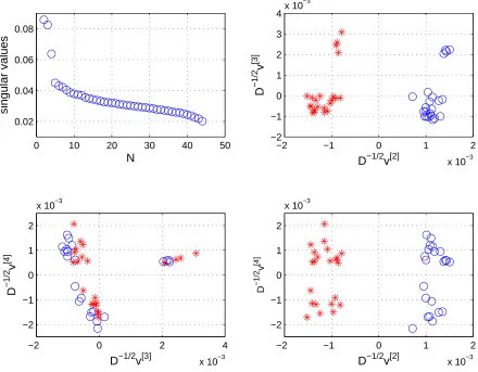
Figures 1 and 3 show N −1 singular values (the first one, σ1 = 1, is
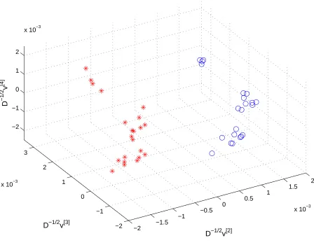
omitted) and scatter plots of pairs of the three dominant singular vectors. In Figure 1, for the colon cancer data, we can see a clear separation of the tumour (stars) and normal (circles) samples by the second, dominant, singu-lar vector. However, the third and fourth singusingu-lar vectors pick out further subgroups. These three singular vectors correspond to the triplet of val-ues separated from the remaining singular valval-ues (top left subfigure). The distinct subclusters may reflect different origins of the samples (laboratory, experiment) or specific features of the patients. Unfortunately, such extra de-tails are not available for these data sets, so this issue cannot be investigated. Figure 2 gives a 3D picture based on the three leading singular values.
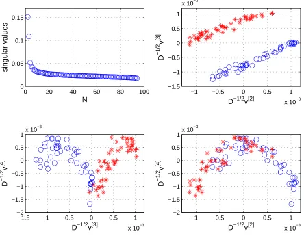
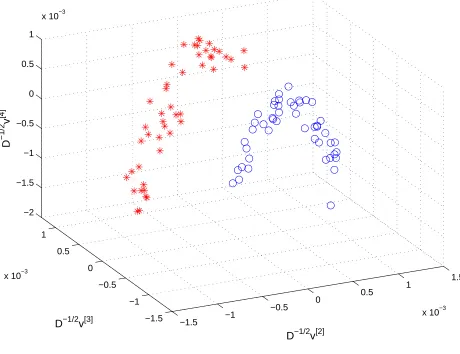
Figure 3 shows an example where tumour and normal samples can be distinguished only by combining singular vectors D−1/2
in v[2] and D
−1/2
in v[3]—
neither singular vector alone gives a perfect separation. A 3D plot of this prostate data set in Figure 4 emphasizes the nonlinear shape of the two clusters.
References
Au-tomation, (1995), pp. 195–200.
[2] S. T. Barnard, A. Pothen, and H. D. Simon,A spectral algorithm for envelope reduction of sparse matrices, Numerical Linear Algebra with Applications, 2 (1995), pp. 317–334.
[3] V. Boginski, S. Butenko, and P. M. Pardalos, On structural properties of the market graph, in Innovations in Financial and Economic Networks, A. Nagurney, ed., Edward Elgar Publishers, 2003, pp. 29–45.
[4] J. P. Brunet, P. Tamayo, T. R. Golub, and J. P. Mesirov,
Metagenes and molecular pattern discovery using matrix factorization, Proc. Nat. Ac. Sci., 101 (2004), pp. 4164–4169.
[5] J. Choi, U. Yu, O. Yoo, and S. Kim,Differential coexpression anal-ysis using microarray data and its application to human cancer, Bioin-formatics, 21 (2005), pp. 4348–4355.
[6] T. F. Cox and M. A. A. Cox, Multidimensional Scaling, Chapman and Hall, London, 1994.
[7] I. S. Dhillon,Co-clustering documents and words using bipartite spec-tral graph partitioning, Proceedings of the Seventh ACM SIGKDD Con-ference, (2001).
[8] C. Ding, X. He, and H. Zha,A spectral method to separate discon-nected and nearly-discondiscon-nected web graph components, in The Seventh ACM SIGKDD International Conference on Knowledge Discovery and Data Mining, ACM, 2001, pp. 275–280.
[9] M. B. Eisen, P. T. Spellman, P.O.Brown, and D.Botstein,
Cluster analysis and display of genome-wide expression patterns, Genet-ics, 95 (1998), pp. 14863–14868.
[10] P. Grindrod, Range-dependent random graphs and their application to modeling large small-world proteome datasets, Physical Review E, 66 (2002), pp. 066702–1 to 7.
[12] D. J. Higham, G. Kalna, and J. K. Vass,Spectral analysis of two-signed microarray expression data, Mathematical Medicine and Biology, to appear.
[13] K. D. Hunter, J. K. Thurlow, J. Fleming, P. J. H. Drake, J. K. Vass, G. Kalna, D. J. Higham, P. Herzyk, D. G. Mac-Donald, E. K. Parkinson, and P. R. Harrison,Divergent routes to oral cancer, Cancer Research, to appear (2006).
[14] D. J. C. MacKay,Information Theory, Inference and Learning Algo-rithms, Cambridge University Press, 2003.
[15] D. Notterman, U. Alon, A. Sierk, and A. Levine, Transcrip-tional gene expression profiles of colorectal adenoma, adenocarcinoma, and normal tissue examined by oligonucleotide arrays, Cancer Res., 61 (2001), pp. 3124–3130.
[16] R. Rifkin, S. Mukherjee, P. Tamayo, S. Ramaswamy, C.-H. Yeang, M. Angelo, M. Reich, T. Poggio, E. S. Lander, T. R. Golub, and J. P. Mesirov, An analytical method for multiclass molecular cancer classification, SIAM Review, 45 (2003), pp. 706–723.
[17] J. Shi and J. Malik, Normalized cuts and image segmentation, IEEE Transactions on Pattern Analysis and Machine Intelligence, 22 (2000), pp. 888–905.
[18] D. Singh, P. Febbo, K. Ross, D. Jackson, J. Manola, C. Ladd, P. Tamayo, A. Renshaw, A. D’Amico, J. Richie, E. Lander, M. Loda, P. Kantoff, T. Golub, and W. Sellers, Gene ex-pression correlates of clinical prostate cancer behavior, Cancer Cell, 1 (2002), pp. 203–209.
[19] R. Van Driessche and D. Roose, An improved spectral bisection algorithm and its application to dynamic load balancing, Parallel Com-puting, 21 (1995), pp. 29–48.
0 10 20 30 40 50 0.02
0.04 0.06 0.08
N
singular values
−2 −1 0 1 2
x 10−3 −2
−1 0 1 2 3 4x 10
−3
D−1/2v[2]
D
−1/2
v
[3]
−2 0 2 4
x 10−3 −2
−1 0 1 2
x 10−3
D−1/2v[3]
D
−1/2
v
[4]
−2 −1 0 1 2
x 10−3 −2
−1 0 1 2
x 10−3
D−1/2v[2]
D
−1/2
v
[image:16.612.116.556.148.491.2][4]
−2 −1.5 −1
−0.5
0 0.5
1
1.5 2
x 10−3
−2 −1 0 1 2 3
x 10−3 −2 −1 0 1 2
x 10−3
D−1/2v[2] D−1/2v[3]
D
−1/2
v
[image:17.612.116.564.161.511.2][4]
0 20 40 60 80 100 0
0.05 0.1 0.15
N
singular values
−1 −0.5 0 0.5 1
x 10−3 −1.5
−1 −0.5 0 0.5 1
x 10−3
D−1/2v[2]
D
−1/2
v
[3]
−1.5 −1 −0.5 0 0.5 1
x 10−3 −2
−1.5 −1 −0.5 0 0.5
1x 10
−3
D−1/2v[3]
D
−1/2
v
[4]
−1 −0.5 0 0.5 1
x 10−3 −2
−1.5 −1 −0.5 0 0.5
1x 10
−3
D−1/2v[2]
D
−1/2
v
[image:18.612.116.560.148.493.2][4]
−1.5 −1
−0.5 0
0.5 1
1.5
x 10−3 −1.5
−1 −0.5 0 0.5 1
x 10−3 −2 −1.5 −1 −0.5 0 0.5 1
x 10−3
D−1/2v[2] D−1/2v[3]
D
−1/2
v
[image:19.612.116.576.162.516.2][4]