Polarization properties in the transition from below to above lasing threshold in broad-area vertical-cavity surface-emitting lasers

Polarization properties in the transition from below to above lasing threshold

in broad-area vertical-cavity surface-emitting lasers

M. Schulz-Ruhtenberg*

Institute for Applied Physics, University of M¨unster, Corrensstrasse 2-4, D-48149 M¨unster, Germany

I. V. Babushkin†

Weierstrass Institute for Applied Analysis and Stochastics, Mohrenstrasse 39, D-10117, Berlin, Germany

N. A. Loiko

Institute of Physics, NASB, 68 Nezalezhnasti Avenue, 220072 Minsk, Belarus

K. F. Huang

Department of Electrophysics, National Chiao Tung University, Hsinchu, Taiwan

T. Ackemann

SUPA and Department of Physics, University of Strathclyde, Glasgow G4 0NG, Scotland, United Kingdom (Received 24 September 2009; published 19 February 2010)

For highly divergent emission of broad-area vertical-cavity surface-emitting lasers, a rotation of the polarization direction by up to 90◦ occurs when the pump rate approaches the lasing threshold. Well below threshold the polarization is parallel to the direction of the transverse wave vector and is determined by the transmissive properties of the Bragg reflectors that form the cavity mirrors. In contrast, near-threshold and above-threshold emission is more affected by the reflective properties of the reflectors and is predominantly perpendicular to the direction of transverse wave vectors. Two qualitatively different types of polarization transition are demonstrated: an abrupt transition, where the light polarization vanishes at the point of the transition, and a smooth transition, where it is significantly nonzero during the transition.

DOI:10.1103/PhysRevA.81.023819 PACS number(s): 42.55.Px, 42.60.Jf, 42.25.Ja, 05.40.−a I. INTRODUCTION

In the past decades vertical-cavity surface-emitting lasers (VCSELs) have played an increasing role in scientific research and applications [1]. One of the features of VCSEL design is the possibility of obtaining large two-dimensional apertures that are quite homogeneous and have a small polarization anisotropy.

The polarization behavior in such lasers resulting from the competition of stimulated and spontaneous emission has been the subject of many investigations [2–6]. It is known that the polarization properties of small- and medium-aperture VCSELs above [7–12] and below [4,5] threshold are deter-mined mainly by the intracavity anisotropies. Well below threshold the polarization degree is reduced dramatically, in VCSELs [4] as well as in edge-emitting semiconductor lasers [13] (which possess much higher intracavity anisotropies). However, below threshold the polarization coincides with the at-threshold one.

As aperture size increases, off-axis emission becomes important. Because the cavity resonance is different for different transverse modes, the off-axis emission with the best alignment between the cavity resonance and the gain maximum of the active medium have the largest gain [14,15]. Recently it was shown [16–18] that for strongly off-axis

*_{Now at Fraunhofer Institute for Laser Technology,} Steinbach-strasse 15, D-52074 Aachen, Germany.

†_{[email protected]}

emission the intracavity anisotropies play only an auxiliary role in polarization selection above threshold. In contrast, the polarization-selective properties of reflection and transmission of the distributed Bragg reflectors (DBRs) forming the cavity mirrors are much more important. Above threshold, the DBR transverse electric (TE) modes (which are in paraxial approximation perpendicular to the transverse component of the wave vector, i.e., s waves) have higherreflectivity, and the cavity quality factor for the TE modes is larger than that for the tansverse magnetic (TM) modes. This determines the polarization of the above-threshold emission, which has an overall tendency to be perpendicular to the transverse wave vector (“90◦ rule”) [17]. It also induces a coupling between polarization and spatial degrees of freedom [18]. A corresponding phenomenon for the eigenmodes of stable dome-shaped microcavities with exact circular symmetry was described in [19,20], leading to a modification and lifting of degeneracies of standard Laguerre-Gaussion modes.

In contrast, in the marginally stable, square plano-planar cavities we are going to discuss, the eigenmodes are better described as a superposition of a few Fourier modes (tilted plane waves). In such geometry, the above-threshold polarization is also strongly affected by the transverse cavity boundaries, that is, the waveguide formed by the oxide confinement [18]. This can lead to strong deviations of the above-threshold polarization state from the 90◦ rule for transverse wave vectors with directions not parallel to either of the device boundaries [18].

the polarization direction for off-axis light is different below and above threshold but there is no detailed investigation. In this work, we characterize the polarization properties of off-axis below-threshold emission and show that the polarization direction is governed mainly by thetransmissiveproperties of the top DBR. The transmissivity is larger for the TM Bragg modes (parallel to the transverse wave vector,pwaves) than for theswaves, resulting in a “0◦rule” for polarization selection; that is, the polarization is parallel to the transverse wave vector. We consider, both theoretically and experimentally, the transition from the below-threshold to the above-threshold polarization state for highly divergent VCSEL emission. The nature of the transition depends critically on the orientation of the polarization of the final (lasing) state. When the final polarization obeys the 90◦ rule and is perpendicular to the polarization state well below threshold, the transition is very abrupt and the light is unpolarized at the point of transition. On the other hand, when the polarization of the final state is not orthogonal to the initial one, the transition is considerably smoother, and the emission retains a relatively large degree of polarization during the transition. Our theory predicts also that far below threshold the main principal axes of the intracavity and extra-cavity field are perpendicular to each other due to the strong anisotropic filtering of the light coupled out via the DBRs.

In the next section we describe the experimental setup. In Sec. IIIthe experimental results are reported. In Sec. IV

a theoretical model for the description of the transition is developed and analyzed and the results compared to the experimental observations. Concluding remarks are in Sec.V.

II. EXPERIMENTAL SETUP AND METHODS The VCSELs under study are oxide-confined top emitters with a square aperture of 40 × 40 µm2 that are packaged in transverse optical (TO)-type housings without caps. The emission wavelength is around 780 nm. The lasers consist of two highly reflective DBRs (top mirror, 31 layers; bottom mir-ror, 47 layers) with three 8-nm-thick Al0.11Ga0.89As quantum wells in between. Together with several Al0.36Ga0.64As spacer layers and the GaAs substrate, the whole structure is about 10µm long. In order to reduce the electrical resistance of the lasers the interfaces between different semiconductor layers are graded. A laterally oxidized layer above the active region provides current and optical confinement.

The devices are electrically pumped with a low-noise DC current source between 0 and 30 mA. The typical lasing threshold at 0◦C heat sink temperature is 15 mA. The VCSEL is mounted on a copper plate that is attached to a thermoelectric cooling element, enabling temperature control between 40◦C and −35◦C. We remark that the actual device temperature is strongly influenced by the driving current due to Joule heating effects. Temperature values given here are for the heat sink only. The device temperature can be inferred indirectly from optical spectra and changes with current by a factor of about 0.9 K/mA. The device temperature changes the detuning between the cavity resonance and the maximum gain frequency, since these shift with distinctly different rates with temperature (typical values are 0.28 nm/K for the gain peak and 0.075 nm/K for the resonance, e.g., [22]). As considered

ND filters CCD camera

mounted VCSEL

Microscope objective

Polarization optics

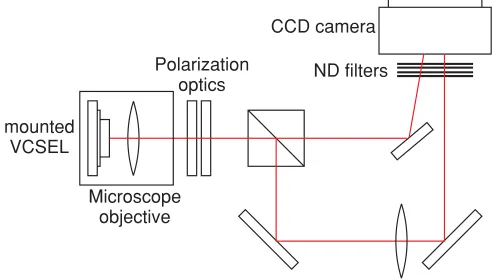
FIG. 1. (Color online) Experimental setup. The VCSEL is set into an air-tight box to avoid condensation water. Polarization optics: half-wave plate and linear polarizer.

in detail in [23], this mechanism controls the length scales of the transverse patterns emitted by the VCSEL.

Figure 1 shows the setup used for the experiments. The laser beam is collimated by a microscope objective with a numerical aperture of 0.8. VCSEL, cooling elements, and the objective are put into an air-tight box to avoid condensation of water at low temperatures. The far field of the laser emission is imaged onto a high-resolution 14-bit camera with a large charge-coupled device (CCD) chip. A half-wave plate and a linear polarizer are inserted into the beam path. The orientation of the polarizer defines the reference coordinate system by which the state of polarization is represented. Horizontal polarization is defined as 0◦and angles are measured in the counterclockwise direction. The polarization is measured by taking far-field images for three settings of the polarization optics: horizontal (Ix), vertical (Iy), and diagonal orientation (I45). For the circular component (Icirc) a quarter-wave plate (set to 45◦ with respect to the horizontal) is necessary. From these data, the spatial-resolved Stokes parameters are calculated,

S0=Ix+Iy, S1=

(Ix−Iy) S₀ ,

S₂=

2I45 S0

−1, S₃=

2Icirc S0

−1, (1)

where S₀ represents the total intensity, S₁ the (normalized) amount of light polarized in thex(positiveS1) ory(negative S1) direction,S2 the (normalized) amount of light polarized along the diagonal direction (positive for 45◦, negative for −45◦_{), andS}

3the (normalized) amount of circularly polarized light (the sign denotes the direction of rotation). Using this set of Stokes parameters, the degree of polarization (fractional polarization) p and the polarization direction ϕ can be calculated:

p=

S₁2+S₂2+S₃2, ϕ= 1 2arctan

S2 S1

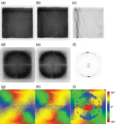
. (2)

III. DISTRIBUTION OF SPONTANEOUS EMISSION AND THE TRANSITION THROUGH THRESHOLD We consider two nominally identical devices from the design and growth process that show however rather different behavior. The near-field and far-field intensity distributions of the emission are shown in Figs. 2 (device 1) and 3

(device 2), respectively. In both cases the heat sink temperature isT =0◦C; the threshold current for device 1 is 15.2 mA and that for device 2 is 15.6 mA. The top and middle rows in each figure depict the intensity distributions in gray-scale coding (black denoting the maximum intensity) of the near-field and far-field, respectively; the third shows the spatial frequency distribution of the polarization direction in a cyclic color code (red denotes±90◦, green−45◦, blue 0◦, and yellow+45◦; cf. the color bar on the right of Fig.2). The columns show the emission below threshold [panels (a), (d), and (g); 12.0 mA for device 1 and 13.5 mA for device 2), slightly below threshold [panels (b), (e), and (h); 13.5 mA for device 1 and 15.5 mA for device 2), and just above threshold [panels (c), (f), (i); 15.6 mA for device 1 and 16.0 mA for device 2). The optical axis is positioned in the center of each image.

Below and above threshold, the emission has its maximum at a well-defined wave number. This critical wave number is favored because it has the most favorable detuning properties, as discussed above (see [23] for details about the dependence of the transverse wave numbers of the emission on the detuning). Even far below threshold the ring indicating the critical wave number is easily discernible. With current approaching

90°

-90° 0° (i)

(g)

(c) (a)

(h)

(f) (d)

(b)

(e)

FIG. 2. (Color online) Near- and far-field images for device 1 below and above threshold. Heat sink temperatureT =0◦C; driving current 12.0 mA (a, d, g), 13.5 mA (b, e, h), 15.6 mA (c, f, i). The color code of the polarization direction distribution (bottom row) is shown by the bar on the bottom right. These images correspond to the transition shown in Fig.5.

90°

-90° 0° (i)

(g)

(c) (a)

(h)

(f) (d)

(b)

(e)

FIG. 3. (Color online) Near- and far-field images for device 2 below and above threshold. Heat sink temperatureT =0◦C; driving current 13.5 mA (a, d, g), 15.5 mA (b, e, h), 16.0 mA (c, f, i). The white spots in panels (a) and (b) result from debris on the neutral density filters. The color code is the same as in Fig.2. These images correspond to the transition shown in Fig.6.

threshold it narrows until at threshold the lasing modes develop from this ring. This is easily explained by the increase of the finesse of the cavity if threshold is approached.

Within this critical ring, far below threshold the maximum of spontaneous emission is found at the diagonals in Fourier space but moves close to the axes above threshold (i.e., with either small kx for device 1 or smallky for device 2). Just above threshold VCSEL 1 emits far-field patterns with two dominant Fourier components on the y axis [Fig.2(f)]. The polarization of these components is in tendency orthogonal to their wave vector, which is shown in Fig. 2(i), where the area of lasing emission is polarized horizontally (blue in the color code). Below threshold the polarization direction is very different, that is, parallel to the wave vector [see Fig.2(g)]. These general observations are also true for device 2.

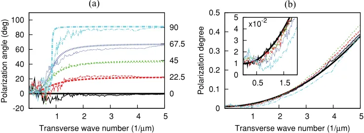
The validity of the 0◦rule is illustrated and tested further in Fig.4. Here radial cuts through the polarization distribution at 0◦, 22.5◦, 45◦, 67.5◦, and 90◦ with respect to the x axis are shown for T =0◦C and I =10 mA (i.e., far below threshold). Each curve starts at about 10◦ for k_⊥≈0 and switches asymptotically to the angle of the cut. For values of the transverse wave number above 1µm−1_{, the polarization is} clearly parallel to the wave number. The deviations amount up to about 10◦at 1µm−1_{and decrease for higher wave numbers.} The polarization state atk_⊥≈0 is interpreted to be selected by the cavity anisotropies.

-20 0 20 40 60 80 100

1 2 3 4 5

0 22.5 45 67.5 90

Polarization angle (deg)

Transverse wave number (1/µm)

(a)

0 0.1 0.2 0.3 0.4 0.5

1 2 3 4 5

Polarization degree

Transverse wave number (1/µm)

(b)

0 1 2 3 4 5

0.5 1.5 x10-2

FIG. 4. (Color online) Radial cuts [at 0◦(black solid line), 22.5◦(red long-dashed line), 45◦(green small-dashed line), 67.5◦(blue dotted line), and 90◦ (cyan dot-dashed line)] through the far-field distribution of the spontaneous emission for device 1.T =0◦C,I=10 mA. (a) Polarization in dependence on the transverse wave numberk⊥showing the validity of the 0◦rule fork⊥>2µm−1_{. The thick lines indicate} the polarization expected from the theory developed in Sec.IV. (b) Fractional polarization in dependence onk_⊥for the same cuts as in panel (a). The part neark_⊥≈0 is shown in the inset.

5 µm−1 _{(depending on the direction of the wave vector) the} cutoff condition for the transverse modes of the waveguide formed by the refractive index step (i.e., the side boundaries formed by oxidation) sets in. It is clearly visible in the center rows of Figs. 2 and 3 that the intensity is cut off indeed. This indicates that the influence of the side boundaries on the polarization characteristics of below-threshold emission is very small.

The fractional polarization, that is, the amount of linearly polarized light, in dependence on the transverse wave number is shown in Fig. 4(b), again for the same cuts. It increases monotonically with wave number. The graphs are more or less congruent, which indicates the isotropic character of the phenomenon, showing its relative independence from the principal axes of the intracavity anisotropy for large-enough wave numbers. The polarization degree is small but nonzero for k_⊥=0 [see inset to Fig.4(b)], which also indicates the influence of the cavity anisotropies, because the DBRs are isotropic fork_⊥=0.

In the following, we take a closer look at the changes involved in the transition from spontaneous to lasing emission. This transition is illustrated in Fig.5for device 1 and Fig.6for device 2. Each figure shows in panel (a) the local (in Fourier

space) intensity, in panel (b) the fractional polarization, and in panel (c) the local polarization orientation in dependence on the driving current. In addition, the pump rate

P =(I −Ith) Ith

(3)

is displayed on the upper x axis of the diagrams. The inset in (a) shows the Fourier component for which these plots were made (indicated by the arrow). The black lines in the Figs.5(a)and6(a)show in both cases the typical behavior of a laser crossing threshold: a region of low emission intensity representing spontaneous emission and small slope, followed by a steeply increasing part indicating lasing emission. Threshold is extrapolated by a linear fit to this latter part and indicated by the dashed red line. The blue dotted curves in Figs.5and6are calculated from Eqs. (9) and (12) and will be discussed in the theoretical section.

The fractional polarization shown in Figs. 5(b)and 6(b)

typically follows the development of the intensity until it saturates at a maximum of 0.8 to 1.0.

In Figs. 5(c) and 6(c), the change of the polarization direction with current is shown. Far below threshold the polarization angle is in good agreement with the 0◦rule. With

FIG. 6. (Color online) Transition from spontaneous emission to lasing emission of the spot depicted in the inset in (a) for device 2. (a) Local intensity in dependence on driving current. (b) Degree of polarization. (c) Local polarization direction. All denotations are analogous to those for Fig.5.

increasing current the scenario is different for the two lasers. For device 1, the polarization starts to change quite abruptly approximately 1.1 mA below threshold: In a current range of only 1 mA, the angle changes to 0◦, which corresponds to the 90◦rule. The polarization reaches the target state well below threshold (about 93% ofIth). Note that the fractional polarization has a pronounced local minimum at the transition. Device 2 [Fig.6(c)] shows a rather gradual change of the polarization that starts already more than 5 mA (at 67 % of Ith) below threshold. The behavior is monotonous; there is no dip in the fractional polarization. This behavior is typical, if the wave vector is not oriented along one of the two axes. Only in the latter case (Fig.5) is an abrupt transition found. The continuous transition is more typical for the devices under study, though, because the wave vector configuration depicted in Fig.6(a)is more typical [18].

IV. THEORY AND DISCUSSION A. The Ginsburg-Landau equation

In order to analyze the behavior described earlier in this article, we use a model for a broad-area VCSEL that accounts for its cavity structure, including Bragg reflectors [17,24]. For simplicity, we consider a spatially homogeneous device with an infinite aperture. For this case the eigenmodes are plane transverse wavesEkt(x, y, t)=E(t) exp{i(kxx+kyy)}, where E(x, y, t)≡ {Ex, Ey} is the slowly varying complex envelope of the field inside the cavity andk_⊥= {kx, ky}is the transverse component of the wave vector.

Many features of polarization selection at and slightly above threshold can be obtained by a linear stability analysis [18,25]. However, for the transition from below to above threshold it is of critical importance to take into account both spontaneous emission and the nonlinear saturation. Therefore, we will use here a nonlinear Ginsburg-Landau equation (GLE) with an additional term describing spontaneous emission (see the Appendix for the derivation). For the spatially homogeneous device with infinite aperture, the equation can be written for every transverse wave with complex amplitudeE(t):

˙

E= −κinE−κoutϒ(k⊥)E+i(k⊥)E+E

−κ_outG(k_⊥)IE+W. (4)

The field decay rate κ =κin+κout results from the laser emission through the DBRsκ_out(outcoupling losses) andκ_in (intracavity losses) by scattering and absorption. The latter is isotropic (polarization independent), whereas the former is anisotropic. The anisotropy is described by the 2×2 matrix ϒ(k_⊥), which represents polarization- and k_⊥-dependent losses at the DBRs. In addition, the matrix ϒ(k_⊥) includes also the gain in the device (and hence has a component depending linearly on the driving current).(k_⊥) represents diffraction in the cavity and in the DBRs, G(k⊥) is a matrix describing the impact of the nonlinear saturation, andI =E†E is the light intensity († means the conjugate transpose). A more detailed description of ϒ(k_⊥), (k_⊥), and G(k_⊥) is given in the Appendix. is the intracavity anisotropy matrix, which in the basis of the main anisotropy axes is written as =diag(γa+iγp,−γa−iγp), where γa is the amplitude anisotropy (dichroism),γp is the phase anisotropy (birefringence), and diag(·,·) denotes a diagonal matrix with the corresponding entities on the diagonals.

As indicated earlier in this article, the other source of anisotropy is the reflection at the DBRs. The action of the DBRs can be described in terms of s and p waves [26,27], which are plane transverse waves with polarization correspondingly perpendicular and parallel to the direction of the transverse wave vector kt. In this basis, the matrix of reflection from theith Bragg reflector is diagonalRi(kt)= diag{Rsi(kt), Rpi(kt)}; that is, puresandpwaves are reflected from the Bragg reflectors without mixing. The correspond-ing transmission matricesTi(kt)=diag{Tsi(kt), Tpi(kt)},i= 1,2, are also diagonal in this basis.

The spontaneous-emission rate is described by the term W≡W(k⊥, t)=βspKj/T1ξ(k⊥, t) in Eq. (4). Here ξ(k_⊥, t) is a Langevin noise source (see the Appendix for details), j is the normalized current density, T1 is the population decay time,β_spis the spontaneous-emission factor (the fraction of spontaneous emission going into the given mode), andK is the Petermann excess quantum noise factor [28], which takes into account a possible nonorthogonality of the modes leading to projection of the noise in other modes onto the selected one [28].

population difference between sub-bands with opposite carrier spin d, cf. Eqs. (A)–(A3)] is neglected. In particular, we assumed equal populations of both sub-bands (d =0). This corresponds to a quasistationary approximation valid for low intensities and linear light polarization (or completely unpolarized light), as motivated by the absence of elipticity in the experimental results. This approximation is fairly good below, directly at, and even slightly above threshold. Of course, when considering the system further above threshold, the population dynamics must be taken into account, which leads to additional nontrivial polarization behavior [7–12], such as polarization switchings. However, the region far above the threshold is beyond the scope of the present article.

B. The coherence matrix

In Eq. (4) the nonlinear term can be neglected for small current well below threshold, which results in the linear equation

˙

E= −κ_inE−κ_outϒ(k_⊥)E+i(k_⊥)E+E+W, (5)

which can be solved directly,

E=exp(t) t

0

exp(−τ)W(τ)dτ, (6)

where= −κin−κoutϒ+i+.

If the field E is known, the Stokes parameters can be obtained from the coherence matrix J = EE† [here · denotes an ensemble (and not time) averaging; note also the reverse order of multiplication in this definition compared to the definition of intensity, which results in a matrix instead of a scalar],

Sj =tr(J σj), (7)

where σj are the Pauli matrices. In particular, the mean intensityI =S₀can be obtained asI =trJ.

By multiplying Eq. (6) from the left with its Hermite conjugate, performing averaging and then integration, we obtain

J = −−_r1JW{1−exp(rt)}, (8)

where r =+† and JW = WW† is the coherence matrix of spontaneous emission. In the derivation of Eq. (8) it is taken into account that the polarization components ofWare δcorrelated and thereforeJWis proportional to the unit matrix JW ij =δijKβspj/2T1 (whereδij,i=1,2 is a Kroneckerδ); that is, it commutes with all other matrices. It is also assumed that all functions of matrix argumentsand†commute.

We will search for the statistically stationary solutions of Eq. (8) (i.e., those with a time-independent coherence matrix). For such solution being finite, the exponential term in Eq. (8) must decay. This is automatically fulfilled below threshold because is nothing but a linear stability matrix for the GLE (4) without noise far below threshold near its nonlasing solution, and therefore all the eigenvalues ofrare less than zero. Hence, for the small current we obtain

J = −−_r1JW. (9)

Equation (9) gives the coherence matrix inside the cavity. Because the Bragg reflectors transmit different polarizations

differently, the coherence matrixJois different fromJ for an observer outside of the cavity:

Jo=T J T†. (10)

Let us turn our attention to the general case of the nonlinear Eq. (4). We can simplify the analysis by neglecting the joint fluctuation of the term IE and replace the intensity with its mean value I in this term. This approximation can be interpreted in the following way: We replace the original stochastic process described by Eq. (4) with a simpler, Gaussian one [29] with the same mean E =0 and, by its construction, with the same stationary mean intensity I. We expect therefore that the stationary coherence matrix J will also not be significantly altered by this approximation. Of course, the process described by the original GLE is not, strictly speaking, Gaussian, especially in the vicinity of threshold or polarization switchings [30,31]. However, as we will see later, this approximation fits rather well to the experimental findings, allowing at the same time very constructive analytical insight. By considering the resulting equation as a linear equation for the field and proceeding as above, we arrive at Eq. (8) with the modified matrix

= −κin−κoutϒ+i−κoutGI +. (11)

As before, we consider only the finite statistically stationary solutions, for which the exponential term in Eq. (8) decays, and obtain again Eq. (9), withgiven now by Eq. (11).

Taking the trace of Eq. (9), one obtains an implicit equation for the intensityI,

I =tr{[2κin+κout(ϒ+ϒ†)−(+†)

+κ_outI(G+G†)]−1JW}, (12) which is a polynomial of third order for I. The intensity outside the cavity is then given byIo =tr{T J T†}. Equation (12) has only one positive root, which is small (I ≈0) below threshold and grows asymptotically linearly with current (I ∼j) above threshold. Below and at threshold it is, however, in rather good agreement with experiment [compare the black and blue curves in Figs.5(a)and6(a)].

C. General features

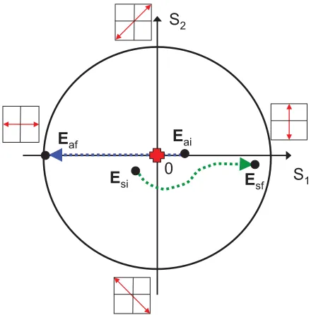
FIG. 7. (Color online) Different types of transitions from nonlas-ing to lasnonlas-ing state in the space of Stokes parameters (S1,S2): abrupt transition (blue straight dashed arrow fromEaitoEaf, corresponds to

device 1) and smooth transition (green curved dashed arrow fromEsi

toEsf, corresponds to device 2). The initial polarization state for the

abrupt transitionEaiis orthogonally polarized to the final oneEaf,

whereas for the initialEsiand finalEsfstates for the smooth transition

this is not the case. For convenience, the polarization directions for different quadrants of the (S1,S2) plane are shown by red arrows in the black boxes. The red cross in the center corresponds to a fully unpolarized state (p=0), whereas the black circle shows the fully polarized state (p=1).

some in another. We are only exploring the consequence of a given wave vector configuration on the polarization behavior. The difference between these two situations can be depicted in the space of Stokes parameters (Fig. 7). Because the polarization is always linear, S₃=0 and we use only its two-dimensional subspace (S₁,S₂). One can see that—if the initial state Eai and the final state Eaf are orthogonal to each other—S2 experiences a zero crossing during the tran-sition (red cross in Fig.7). According to Eq. (2), this means that the degree of polarization is also zero at the crossing point. The polarization direction retains only two values during this transition. Hence the transition, which appears at the point S1=S2=0, is an abrupt switching between two discrete polarization states. Both the transition of the degree of polarization through zero and the abrupt switching can be seen in Figs.5(b)and5(c). On the other hand, when the final stateEsfis not orthogonal to the initial oneEsi, the polarization follows a path avoiding the origin; that is, it rotates to the final state instead of switching to it. In this case, the degree of polarization does not pass through zero and the polarization direction changes smoothly [see Figs.6(b)and6(c)].

We will refer to the first case as an “abrupt” transition and to the second case as a “smooth” one. One can see a remote analogy to the Ising and Bloch transitions [32], which also represent abrupt “switching” or smooth “rotating” behavior. The role of the vector of magnetization in this case is played by the Stokes parameters. One should note, however, that

Ising and Bloch transitions occur in space, that is, between energetically equivalent spatially separated states (at constant external parameters), whereas here the transition takes place in dependence on an external parameter (current), that is, in the parameter space.

The previously mentioned difference between the abrupt and smooth transitions can be expressed more directly in terms of the coherence matrix. For the abrupt transition, the coherence matrix is diagonal inone and the same coordinate basis during the whole transition. Only two polarization directions are possible, depending on which diagonal element, J₁₁ or J₂₂, is larger. The point representing the polarization state in Fig. 8 can move only along a straight line passing through zero (S1=0, S2=0). At the point of transition J11=J22; that is, the light is unpolarized, and the polarization direction changes abruptly. In the case of a smooth transition, the situation is different. Of course, the coherence matrix is Hermitian and therefore there is always a Cartesian coordinate basis in which it is diagonal. However, this basisis changing during the transition. That reflects the existence of several competing mechanisms (DBRs, side boundaries, intracavity anisotropies), each of them having its own principal axes. Their mutual influence is changing with a change of parameter (here current). In this case, the Stokes parameters do not vary along a straight line and can avoid the zero crossing. It should be noted also that the origin (S1=0,S2=0) is a special point in the sense that the coherence matrix in this point is proportional to the identity matrix and therefore is diagonal in every coordinate basis.

D. Detailed discussion

The polarization, intensity and fractional polarization ob-tained from Eqs. (9), (10), and (12) are shown in Figs.4,5, and 6 in comparison to experimental data. The parameters of the active layer and the cavity used for calculations are α=3,γ =103_ns−1_,γ

a =0.8 ns−1, andγp =0. The DBRs, consisting of 31 (top mirror) and 47 (bottom mirror) λ/4 layers of material with alternating refractive indexn₁=3.46, n2 =3.093 and the transparency current Jtr =7 mA were assumed. The effective round-trip time τ =33 fs includes also the effects of the dispersion in the DBRs and in the cavity [23]. The outcoupling loses for these parameters are κ_out=17.4 ns−1_{. The best coincidence with the experimental} results appears for κin=65 ns−1, which is in rather good agreement with estimations based on losses in the p-DBR and typical gain values of GaAs quantum wells [33,34].

0 1 2 3 4

1 2 3 4 0

50 100 150

γba

(1/ns)

γbp

(1/ns)

Transverse wave number (1/µm) (a)

0 0.02 0.04 0.06 0.08 0.1 0.12 0.14 0.16

1 2 3

Polarization degree

Transverse wave number (1/µm) (b)

-20 0 20 40 60 80 100

1 2 3 4

Polarization angle (deg)

Transverse wave number (1/µm) (c)

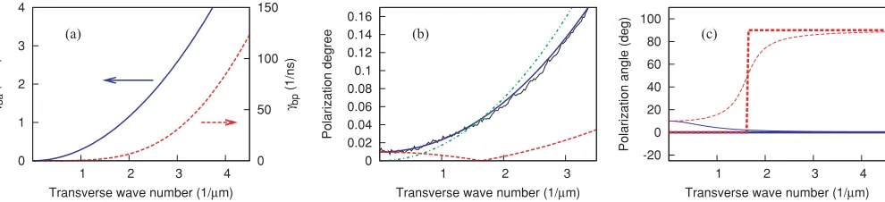
FIG. 8. (Color online) (a) The amplitudeγba (blue solid line) and phaseγbp(red dashed line) anisotropy induced by the Bragg reflector. (b) The degree of polarization for the parameters of device 1 (see Fig.4) andky =0 according to theoretical calculations. The polarization degree inside the cavity is indicated by the red dashed line, that outside the cavity by the blue solid line. The corresponding experimental curve is depicted by the black thin line. The extracavity polarization in the “pure filtering limit” (i.e., assuming completely unpolarized light inside the cavity) is indicated by the green dot-dashed line. (c) The polarization direction inside (red dashed lines) and outside (blue solid lines) the cavity for the intracavity anisotropy favoringxpolarization [thick lines, as in panel (b)] or an anisotropy favoring a polarization direction of 10◦(thin lines).

angle of rotation is 25◦, which corresponds approximately to the angle of the wave vectors visible in the inset of Fig.3(a).

Although the spontaneous-emission factor is rather small (β_sp≈10−5_{) for VCSELs with a transverse size around} 40µm [35], it can be significantly enhanced by the Petermann excess factor. The value of K depends extremely strongly on the inhomogeneities and imperfections in the construction of a particular device. The best results in comparison to experiment give the values Kβ_sp=6×10−4 _{for device 1} and Kβ_sp=10−2 _{for device 2. In [18] it is shown that} the four spots at the corners of a rectangular that form the dominant Fourier peaks of the spatial structures [see inset of Fig.6(a)] can form the eigenmode of the transverse waveguide but are not simultaneously an eigenmode of the reflection operator of the DBR. Thus, the reflection couples many transverse wave vectors k_⊥. This may be the the origin of the rather large Petermann factorK, especially for device 2. In addition, nonorthogonality of the modes might originate from inhomogeneities of the structure and current distribution [which is clearly visible in the intensity distributions in Figs.2(a)–2(c)and3(a)–3(c)for devices 1 and 2].

With this choice of parameters, a very good agreement between experiment and theory is obtained for the develop-ment of the fractional polarization and the local polarization direction versus current for both devices (Figs.5and6), as well as for the dependence on the transverse wave vector (Fig.4). The data reflect the degree of abruptness of the transition [Fig.

5(c) vs Fig. 6(c)] and the monotonous vs nonmonotonous development of fractional polarization [Fig.6(b)vs Fig.5(b)]. The increase of fractional polarization and the convergence toward the 90◦rule with increasing wave number is due to the increasing anisotropy betweensandpwaves, of course [see the blue line in Fig.8(a)].

The case of the abrupt transition allows more analytical insight. Let us suppose for the sake of clarity that the isotropic intracavity anisotropy is diagonal in the representation ofsand pwaves. In this situation, all the matrices in Eqs. (9) and (10) are diagonal in this representation. Therefore, the coherence matricesJ,Joare also always diagonal. In this case, Eqs. (9) and (10) are decoupled into independent equations for the

diagonal elements,

Jii =

Kβspj

2T1[κin+κoutRe(ϒii)+Re(ii)+κoutIRe(Gii)] ,

Joii = |Tii|2Jii, (13)

wherei=1 corresponds to the DBRswave andi=2 to the pwave.

Well below threshold the denominator in Eq. (13) is positive and approximately the same for bothsandpwaves (as will be discussed later in this article), and the light outside of the cavity is slightly p polarized (Jo11< Jo22) due to the filtering by the Bragg reflector. As the current approaches threshold, the denominator for thes wave in Eq. (13) tends to zero, whereas the one for the p wave remains positive, which provides superiority for theswave strongly overcoming the opposite difference in transmission. Obviously, at some point the transition between s and p polarization occurs. At the point of transitionJo11 =Jo22 (and thereforeS1 =0, S₂=0); that is, the output is unpolarized [see Fig. 7, blue straight arrow, and Fig.5(b)]. Because the coherence matrix is diagonal, the polarization direction can have only two values, corresponding to eitherJo11 < Jo22 (0◦ rule) or Jo11> Jo22 (90◦ rule). Therefore, at the transition point, the polarization direction changes abruptly and is constant in all other points above and below threshold [see Fig.5(c)].

Let us now consider the behavior of the extracavity polar-ization far below threshold [when the intensity-dependent term in Eq. (13) can be neglected]. If we suppose that the intracavity lossesκ_in are much larger than the ones through outcoupling κ_out and much larger than the intracavity anisotropyii, we obtain

Jii = Kβ_spj 2T1κin

, Joii = |Tii|2Jii. (14)

degree of polarization is determined only by the transmitting properties of the Bragg reflector [see Fig. 8(b), green dot-dashed line]. The difference in transmission betweens and p waves increases withk_⊥ approximately quadratically, and the degree of polarization in this case reflects this dependence according to Eq. (14).

For the opposite case,κ_outκ_in and assuming a diagonal coherence matrix, we obtain

Joii ∼ |Tii|2/Re(ϒii), (15)

instead of Eq. (14). Because for small current ϒii∼1− |Rii|2= |Tii|2, the light outside the cavity is completely unpolarized in this case. This is in agreement with the energy conservation principle, since the numbers of intracavity photons in both polarizations are increased by the spontaneous emission equally and the polarizations do not mix. Therefore, in the stationary case, in the absence of intracavity losses the energy escaping the cavity must also be equal for both polarizations.

In general, the extracavity polarization degree, defined by Eq. (13), lies between these two limiting cases [Fig. 8(b), thick, solid blue line]. As the Bragg reflection is isotropic for k_⊥=0 (ϒii|k_⊥=0=1 for i=1,2), the polarization for k_⊥≈0 is defined only by the intracavity amplitude anisotropy γa (and does not depend on γp). The best agreement with the experimental value of the degree of polarization for k_⊥=0 is achieved for γa =0.8 ns−1, a reasonable number in line with typical observations in small-area VCSELs [36,37]. With increasing transverse wave numberk_⊥, the relative importance of the anisotropy induced by ϒ(k_⊥) increases. The amplitude anisotropy γba(k⊥)= κ_out{Re[ϒ₁₁(k_⊥)]−Re[ϒ₂₂(k_⊥)]}/2 and the phase anisotropy γbp(k⊥)=κout{Im[ϒ11(k⊥)]−Im[ϒ22(k⊥)]}/2, induced by ϒ(k⊥) are shown in Fig. 8(a). In analogy to the intracavity anisotropy, onlyγbaplays a role in determining the coherence matrix. As one can see,γbaincreases approximately quadrat-ically with k_⊥. The degree of polarization insidethe cavity [see Fig. 8(b), thick dashed red line] is influenced more strongly by the intracavity anisotropy for small k_⊥ (below ∼1.5µm−1) and by the Bragg-induced anisotropy for larger k_⊥. However, it remains relatively small for allk_⊥, and the polarization degree outside of the cavity is therefore quite strongly determined by the Bragg filtering mechanism [see Fig.8(b), thick solid blue line].

Now let us consider the behavior of the polarization of the intracavityfield in dependence onk_⊥far below threshold in more detail. As an example, a cut displaying the polarization angle along thekx axis, assuming the anisotropy also being directed along the x axis, is shown in Fig. 8(c). In this case, the intracavity and extracavity light for k_⊥≈0 is x polarized. However, for high-enoughk_⊥(above≈1.5µm−1_), the DBR-induced anisotropy overcomes the intracavity one and the intracavity light becomes weakly polarized in the directionperpendiculartok_⊥[see Fig.8(c), thick red dashed line]. This degree of polarization is small and canceled when the light is transmitted through the Bragg reflector. Hence, the polarization of the light outside of the cavity is still determined by the transmission, that is, is paralleltok_⊥, as mentioned previously [see Fig.8(c), blue lines].

Hence, we also encounter a polarization transition in the intracavity field if we considerk_⊥ as a parameter instead of the current. This transition is abrupt [see Fig.8(c), thick red dashed line] and the fractional polarization vanishes at the transition point [see Fig.8(b), thin red dashed line]. It can be understood in a way fully analogous to the abrupt transition appearing with the change of current. It should be noted that this transition is not apparent outside the cavity [thick blue line in Fig.8(c)].

This behavior becomes slightly more complex if one analyzes the polarization along a cut in Fourier space whose direction does not coincide with the preferred intracavity anisotropy axis. In that case, the change of polarization angle vs wave number is smooth [Fig.8(c), thin red dashed line] and also detectable outside the cavity [Fig. 8(c), thin blue line]. This is backed up by the experimental curves displayed in Fig. 4(a), where the transition is most notable for the cyan curve, which corresponds to a cut along 90◦; that is, the competition between intracavity anisotropy and Bragg anisotropy is more apparent in the extracavity polarization, if the deviation between wave vector and anisotropy angle increases.

V. CONCLUSION

For highly divergent emission in wide-aperture VCSELs, the polarization direction is determined by the properties of the DBRs and (close to threshold) by the transverse structure of the cavity. Far below threshold the polarization is independent from the cavity structure and thepwave of the DBRs (which has the polarization direction parallel to k_⊥) prevails in the emission because the almost unpolarized intracavity light is filtered by the transmission through the DBR, which is higher for p waves than for s waves. In the simplest case, when the above-threshold polarization direction is not strongly influenced by the transverse boundaries, an abrupt switch of polarization direction occurs as the current increases toward the laser threshold: theswave inside the cavity starts to prevail because the reflectivity and therefore the quality factor of the cavity is higher than the one for thepwave. At the point of transition the filtering effect of the transmission through the DBR cannot compensate the intracavity polarization anymore, and the polarization changes its direction from the one parallel tok_⊥to the perpendicular one. This abrupt change of polarization direction is accomplished by the passing through zero of the degree of polarization of the light outside of the cavity.

On the other hand, if the above-threshold polarization does not coincide with the DBR s mode, the transition is qualitatively different. In this case, the polarization changes smoothly and the degree of polarization is significantly nonzero during the entire transition. As was shown in [18], the deviation of the above-threshold polarization direction from the one dictated by theswave of the DBRs can be due to the influence of the side boundaries of the cavity.

are possible. If the different mechanisms influencing the polarization have different directions, the resulting coherence matrix is nondiagonal and arbitrary polarization direction is possible.

We note an analogy between the abrupt and smooth transi-tions described here and Ising and Bloch transitransi-tions between two equivalent states in ferromagnetics with respect to a “switching” vs “rotation” behavior. However, the polarization transition in this article occurs in parameter space (between energetically inequivalent states) in contrast to the usual Bloch and Ising ones.

ACKNOWLEDGMENTS

We acknowledge financial support from the Deutsche Forschungsgemeinschaft, the Deutsche Akademische Aus-tauschdienst, and the Taiwanese Research Council (Grant No. NSC-96-2112-M-009-027-MY3) at the initial stages of the work.

APPENDIX: THE GINSBURG-LANDAU EQUATION A. The initial equations

Polarization phenomena in VCSEL are often modeled using an equations for the intracavity field Eand the total carrier density D, as well as the population difference d between sub-bands with opposite carrier spin [7,17]. We start from the nonlinear Eqs. (18) of [17] for the normalized complex-valued envelopeE(t,k_⊥) of the optical field for givenk_⊥and carrier population variablesD,d:

˙

E= −κ_outME−iE−iκ_outαE

+κout(1+iα)G(AE)+W, (A1) ˙

D= −γ₁{D−j +Im[(i−α)E∗L(AE)]}, (A2) ˙

d = −γsd−γ1Re[(i−α)E∗L(AE)]. (A3)

Here α is the linewidth enhancement factor, j is the normalized current density,κoutis the outcoupling losses (see later in this article),γ₁=1/T₁andγsare the decay rates ofD

andd, respectively,E= {Ey,−Ex}, andA=( D id −id D). The linear operators M(k_⊥),(k_⊥),G(k_⊥), andL(k_⊥) describe the losses, diffraction, and gain in the cavity and are 2×2 k_⊥-dependent matrices acting on the vector fieldE(k_⊥).

In the present article we assume that(k⊥)= −k2_⊥v/k0I+ [s1(k⊥)+s2(k⊥)]/τ is a matrix describing the dispersion relation given by the cavity resonance condition for s and p waves of DBR. Herev is the speed of light in the cavity, k₀ is the longitudinal part of the wave vector,τ is the cavity round-trip time, I=diag(1,1) [diag(·,·) is here a diagonal matrix with corresponding entities on the diagonals], ands1, s2 are the matrices describing diffraction of the light in the DBRs. Ins-prepresentation, they can be written assi =diag(ssi, spi), wherei=1,2 andssi,spiare the phase shift forsandpwaves. Using these assumptions, M(k_⊥) and G(k_⊥) can be written in terms of propagation matrices F1(k⊥)= (ρ˜)1/2R1(k⊥) exp[−is1(k⊥)], F2(k⊥)=(ρ˜)1/2R2(k⊥) exp

[−is2(k⊥)],F =F1F2:M(k⊥)=[1−F(k⊥)]/M0, G(k⊥)=

[1+F1(k⊥)+F2(k⊥)+F(k⊥)]L/G0. M and G are nor-malized by the constants M₀ and G₀ in such a way that

M₁₁(0)=1 and G₁₁(0)=1. Here R(kt) is an operator describing the reflection from the Bragg mirrors, represented by matricesRm=Rmij(m=1,2,i=1,2,j =2,2).κout= [1− |R111(0)||R211(0)|]/τ =[1− |R122(0)||R222(0)|]/τis the outcoupling losses for zero transverse mode.ρ describes all intracavity losses in the whole system (which are not due to outcoupling) and ˜is the intracavity anisotropy matrix, which in the basis of the main anisotropy axes is written as

˜

=

exp(γaτ +iγpτ) 0

0 exp(−γaτ −iγpτ)

, (A4)

where γa is the amplitude anisotropy andγp is the birefrin-gence. The influence of the gain contour lineL(k_⊥) is given by the expressionL=1/{1+[(δ−)/γ]2_{}, whereLis the} cavity length andγ is the material polarization decay rate.

The spontaneous emission is described by the termW=

Kβspγ1Dξ in the approximation of zero inter-sub-band population difference. Here, K is the Petermann excess quantum noise factor and βsp is the spontaneous-emission factor. ξ is the Langevin noise source with zero mean and correlation in (x, y) space and circular wave basisξ(x, y, t)= [ξ₊(x, y, t), ξ₋(x, y, t)]:

ξ_±(x, y, t)ξ_±(x, y, t) =2δ(t−t)δ(x−x)δ(y−y), ξ_±(x, y, t)ξ_∓(x, y, t) =0. (A5) Performing the transverse Fourier transform and transforming into a basis of linear (orthonormal) polarization with arbitrary directions of axes 1 and 2,one obtains the analogous equation forξ(kx, ky, t)=[ξ1(kx, ky, t), ξ2(kx, ky, t)]:

ξj(kx, ky, t)ξi(kx, ky, t)

=2δijδ(t−t)δ(kx−kx)δ(ky−ky). (A6) Therefore, the noise is also correlated in thek_⊥representation and in an arbitrary orthogonal polarization basis. The noise terms in the equations forDanddare neglected in the present consideration.

B. The derivation of the Ginsburg-Landau equation for the field Here we obtain the lowest-order nonlinear equations for the field resulting from the previously mentioned nonlinear equations. We take into account that near lasing threshold the resulting linear operator acting on E, D, and d has a block-diagonal form with the part acting on E not being coupled to the carrier part. The eigenvalues stemming from the carrier-related part are always strongly negative. In addition, d =0 for linearly polarized (or unpolarized) light. The absence of circularly polarized components is validated by the experimental results presented in Sec.II. Then it is possible to adiabatically eliminateD and obtain a complex equation for Eonly.

The solution of ˙D=0 is given then byD=j/(1+IL), whereI = |E|2_{. For small intensityI one can write it asD∼} j(1−IL). Substituting this into the equation for the field, we obtain

˙

E= −κoutME−iE−iκoutαE+κout(1+iα)j GLE

Because the anisotropy and the intracavity losses are small compared to 1, the corresponding terms can be de-composed asρ=exp(−κinτ)≈1−κinτ, ˜≈1+τ, with =diag(γa+iγp,−γa−iγp). Consideringκinτ,κoutτ, and τ as small parameters and neglecting these terms starting from the first order inGand from the second order inMand introducing the matricesG=(1+iα)jG˜L2_{,ϒ =M˜ +iα−}

(1+iα)jG˜L (where ˜M=M|_ρ=1,˜=1, ˜G=G|ρ=1,˜=1), we obtain the resulting GLE (4).

The spontaneous-emission term in the approximation of a small intensity can be written as W(k⊥, t)=

Kβspγ1jξ(k⊥, t). Here we neglected the second-order term

in the decomposition of the stationary value of D into a series.

[1] C. Wilmsen, H. Temkin, and L. A. Coldren, Vertical-Cavity Surface-Emitting Lasers(Cambridge University Press, Cambridge, 1999).

[2] J. Mulet, C. R. Mirasso, and M. San Miguel, Phys. Rev. A64, 023817 (2001).

[3] J.-P. Hermier, M. I. Kolobov, I. Maurin, and E. Giacobino, Phys. Rev. A65, 053825 (2002).

[4] M. B. Willemsen, A. S. v. d. Nes, M. P. v. Exter, J. P. Woerdman, M. Kicherer, R. King, R. J¨ager, and K. J. Ebeling, J. Appl. Phys. 89, 4183 (2001).

[5] D. Shelly, T. Garrison, M. K. Beck, and D. Christensen, Opt. Express7, 249 (2000).

[6] Y. M. Golubev, T. Y. Golubeva, M. I. Kolobov, and E. Giacobino, Phys. Rev. A70, 053817 (2004).

[7] M. SanMiguel, Q. Feng, and J. V. Moloney, Phys. Rev. A52, 1728 (1995).

[8] M. Travagnin, M. P. vanExter, A. K. Jansen vanDoorn, and J. P. Woerdman, Phys. Rev. A54, 1647 (1996).

[9] M. Travagnin, Phys. Rev. A56, 4094 (1997).

[10] M. Sondermann, M. Weinkath, T. Ackemann, J. Mulet, and S. Balle, Phys. Rev. A68, 033822 (2003).

[11] S. Balle, E. Tolkacheva, M. S. Miguel, J. R. Tredicce, J. Mart´ın-Regalado, and A. Gahl, Opt. Lett.24, 1121 (1999).

[12] K. Panajotov, B. Nagler, G. Verschaffelt, A. Georgievski, H. Thienpont, J. Danckaert, and I. Veretennicoff, Appl. Phys. Lett.77, 1590 (2000).

[13] A. A. Ptashchenko and F. A. Ptashchenko, Solid-State Electron. 39, 1495 (1996).

[14] J. V. Moloney and A. C. Newel, Physica D44, 1 (1990). [15] P. K. Jakobsen, J. V. Moloney, A. C. Newell, and R. Indik, Phys.

Rev. A45, 8129 (1992).

[16] S. P. Hegarty, G. Huyet, J. G. McInerney, and K. D. Choquette, Phys. Rev. Lett.82, 1434 (1999).

[17] N. A. Loiko and I. V. Babushkin, J. Opt. B3, S234 (2001). [18] I. V. Babushkin, M. Schulz-Ruhtenberg, N. A. Loiko,

K. F. Huang, and T. Ackemann, Phys. Rev. Lett.100, 213901 (2008).

[19] D. H. Foster and J. U. N¨ockel, Opt. Lett. 29, 2788 (2004).

[20] D. H. Foster, A. K. Cook, and J. U. N¨ockel, Phys. Rev. A79, 011803 (2009).

[21] M. Schulz-Ruhtenberg, Y. Tanguy, R. J¨ager, and T. Ackemann, Appl. Phys. B97, 397 (2009).

[22] S. P. Hegarty, G. Huyet, P. Porta, J. G. McInerney, K. D. Choquette, K. M. Geib, and H. Q. Hou, J. Opt. Soc. Am. B 16, 2060 (1999).

[23] M. Schulz-Ruhtenberg, I. Babushkin, N. A. Loiko, T. Ackemann, and K. F. Huang, Appl. Phys. B81, 945 (2005).

[24] N. A. Loiko and I. V. Babushkin, Quantum Electron.31, 221 (2001).

[25] I. V. Babushkin, N. A. Loiko, and T. Ackemann, Phys. Rev. E 69, 066205 (2004).

[26] M. Born and E. Wolf,Principles of Optics(Pergamon, Oxford, 1980).

[27] D. I. Babic, Y. Chung, N. Dagli, and J. E. Bowers, IEEE J. Quantum Electron.29, 1950 (1993).

[28] K. Petermann, IEEE J. Quantum Electron.15, 566 (1979). [29] C. W. Gardiner,Handbook of Stochastic Methods for Physics,

Chemistry, and the Natural Sciences (Springer, New York, 2004).

[30] L. Mandel and E. Wolf,Optical Coherence and Quantum Optics (Cambridge University Press, Cambridge/New York/Australia, 1995).

[31] G. Giacomelli and F. Marin, Quantum Semiclass. Opt.10, 469 (1998).

[32] P. Coullet, J. Lega, B. Houchmanzadeh, and J. Lajzerowicz, Phys. Rev. Lett.65, 1352 (1990).

[33] D. I. Babic, J. Piprek, K. Streubel, R. P. Mirin, N. M. Margalit, D. E. Mars, J. E. Bowers, and E. L. Hu, IEEE J. Quantum Electron.33, 1369 (1997).

[34] L. A. Coldren and S. W. Corzine,Diode Lasers and Photonic Integrated Circuits(Wiley, New York, 1995).

[35] J. H. Shin, H. E. Shin, and Y. H. Lee, Appl. Phys. Lett.70, 2652 (1997).

[36] M. P. van Exter, A. Al Remawi, and J. P. Woerdman, Phys. Rev. Lett.80, 4875 (1998).