On optimal solution error covariances in variational data assimilation problems

On optimal solution error covariances in variational data

assimilation problems

I.Yu. Gejadze

a

_{, F.-X. Le Dimet}

b

_{, V. Shutyaev}

c,_*

a_{Department of Civil Engineering, University of Strathclyde, 107 Rottenrow, Glasgow G4 ONG, UK}

b_{MOISE Project (CNRS, INRIA, UJF, INPG); LJK, Université Joseph Fourier, BP 51, 38051 Grenoble Cedex 9, France} c_{Institute of Numerical Mathematics, Russian Academy of Sciences, 119333 Gubkina 8, Moscow, Russia}

The problem of variational data assimilation for a nonlinear evolution model is formulated as an optimal control problem to find unknown parameters such as distributed model coef-ficients or boundary conditions. The equation for the optimal solution error is derived through the errors of the input data (background and observation errors), and the optimal solution error covariance operator through the input data error covariance operators, respectively. The quasi-Newton BFGS algorithm is adapted to construct the covariance matrix of the optimal solution error using the inverse Hessian of an auxiliary data assim-ilation problem based on the tangent linear model constraints. Preconditioning is applied to reduce the number of iterations required by the BFGS algorithm to build a quasi-Newton approximation of the inverse Hessian. Numerical examples are presented for the one-dimensional convection–diffusion model.

1. Introduction

The methods of data assimilation (DA) have become an important tool for analysis of complex physical phenomena in various fields of science and technology. These methods allow us to combine mathematical models, data resulting from instrumental observations and a priori information. The problems of variational DA can be formulated as optimal control problems (e.g.[10,12]) to find unknown model parameters such as initial and/or boundary conditions, right-hand sides in the model equations (forcing terms), and distributed coefficients. A necessary optimality condition reduces an optimal con-trol problem to an optimality system which includes inexact input functions; hence the error in the optimal solution. In this paper, assuming a perfect model, we consider two types of input errors: the background error and the observation error. It is an important theoretical and practical task to evaluate statistical properties of the optimal solution error. For example, its covariance can be used for estimating the efficiency of DA in terms of reducing uncertainty in model parameters and, there-fore, in the model output.

The error in the optimal solution can be derived through the errors in the input data using the Hessian of an auxiliary DA problem[6,11]. If errors in the input data are random and subjected to the normal distribution, then for a linearized finite-dimensional problem (tangent linear approximation of the discretized model) the covariance matrix of the analysis (optimal estimation of the initial condition) error is given by the inverse of the Hessian matrix of the cost functional (see e.g.

of the auxiliary DA problem based on the tangent linear model (TLM) constraints. We have also demonstrated that this approximation could be sufficiently accurate even though the tangent linear hypothesis is not valid.

This paper presents a generalization of the theoretical results reported in[6]to parameter estimation problems for a non-linear evolution model. These problems are common inverse problems considered in geophysics[20,25]and in engineering applications[1]. Here we derive the relationship between the optimal solution error covariance and the inverse Hessian of the auxiliary DA problem in a continuous operator form. The algorithm based on the quasi-Newton BFGS method (also re-ported in[6]) is adapted for constructing the optimal solution error covariance matrix for parameter estimation problems. This process is greatly accelerated by preconditioning the Hessian of the auxiliary DA problem, whereas the preconditioner is also defined in a general operator form.

For numerical analysis we use the one-dimensional (1D) nonlinear convection–diffusion model. The algorithm was ap-plied to compute the covariance matrix for the diffusion coefficient and boundary flux estimation problems. The numerical results reveal interesting features of these problems in terms of identifiability, even for a simple evolution model. All numer-ical results have been verified using the fully nonlinear ensemble method[6]. Thus, we confirm that in the nonlinear case the optimal solution error covariance can be approximated by the inverse Hessian of the auxiliary DA problem (‘H-covariance’) beyond the validity of the tangent linear hypothesis.

The generalization of the theoretical results to the case of model errors is given in[19]. The relevant work discussing an estimate of posterior error fields in DA is given in[18].

This paper is organized as follows. In Section2, we give the statement of the variational DA problem for a nonlinear evo-lution model to estimate the model parameters. In Section3, the equation for the optimal solution error is derived through the errors of the input data. In Section4we derive the formulas for the optimal solution error covariance operator through the covariance operators of the input data errors using the Hessian of the auxiliary DA problem. A general case is considered in Section4.1. Then, it is illustrated by the examples given for the 1D convection–diffusion model: the diffusion coefficient estimation problem is considered in Section4.2and the boundary flux estimation problem in Section4.3. Details of numer-ical implementation are presented in Section5(for basic implementation details we also refer to[6]). We describe: in Sec-tion5.1a method for specifying the background error covariance matrix, in Section5.2– the preconditioning of the Hessian of the auxiliary DA problem and in Section5.3– other relevant implementation issues. Numerical analysis is presented in Section6. In Section6.1we analyse the diffusion coefficient estimation problem, in Section6.2– the boundary flux estima-tion problem. In Secestima-tion6.3we compare the convergence rates achieved with and without preconditioning for some numer-ical tests performed earlier. The main results are discussed in the Conclusions.

From this point on we shall refer to ‘optimal solution error covariance/variance’ simply as ‘covariance/variance’.

2. Statement of the problem

Consider the mathematical model of a physical process that is described by the evolution problem

@u

@t ¼Fð

u

;kÞ þf; t2 ð0;TÞ;

u

jt¼0¼u;

(

ð2:1Þ

where

u

¼

u

ðt_Þis the unknown function belonging for anytto a Hilbert spaceX;u₂X;Fis a nonlinear operator mapping

YYp into Y with Y¼L2ð0;T;XÞ;k kY¼ ð;Þ

1=2

Y ;Yp is a Hilbert space (space of control parameters, or control space), f 2Y. Suppose that for givenu2X;f 2Y andk2Ypthere exists a unique solution

u

2Yto(2.1). The functionkis an

un-known model parameter.

Let us introduce the functional

S_ðk_{Þ ¼}1

2ðV1ðkkbÞ;kkbÞYpþ 1

2ðV2ðCu

u

obsÞ;Cu

u

obsÞYobs; ð2:2Þ

wherekb2Ypis a prior (background) function,

u

obs2Yobsis a prescribed function (observational data),Yobsis a Hilbert space

(observation space),C:Y_!Yobsis a linear bounded observation operator,V1:Yp!Yp andV2:Yobs!Yobsare symmetric

positive definite bounded operators.

Let us consider the following DA problem with the aim to estimate the parameterk: for givenu₂X;f ₂Y, findk2Ypand

u

2Ysuch that they satisfy(2.1), and on the set of solutions to(2.1), the functionalS_ðkÞtakes the minimum value, i.e. @u

@t ¼Fð

u

;kÞ þf; t2 ð0;TÞ;

u

jt¼0¼u;

S_ðkÞ ¼_vinf 2Yp

S_ð

v

Þ: 8

> > < > > :

ð2:3Þ

We suppose that the solution of(2.3)exists. Let us note that the solvability of the parameter estimation problems (or iden-tifiability) has been addressed, e.g., in[2,14]. To derive the optimality system, we assume the solution

u

and the operator

F_ð

u

;k_Þin(2.1) and (2.2)are regular enough, and for

v

₂Y_pfind the gradient of the functionalSwith respect tok:

S0

ðk_Þ

v

¼ ðV₁ðkk_bÞ;

v

Þ_Y

pþ ðV2ðCu

u

obsÞ;C/ÞYobs ¼ ðV1ðkkbÞ;

v

ÞYpþ ðC _V

where/is the solution to the problem:

@/

@t ¼F 0

uð

u

;k_Þ/_þF0

kð

u

;kÞ

v

; t2 ð0;TÞ;

/_jt¼0¼0;

(

ð2:5Þ

HereF0_uð

_u

_{;kÞ:Y ! Y; F}0

kð

u

;kÞ:Yp ! Yare the Frechet derivatives ofFwith respect to

u

andk, correspondingly, andCis

the adjoint operator toCdefined byðC

u

;w_ÞY

obs ¼ ð

u

;C _wÞ

Y;

u

2Y; w2Yobs.

Let us consider the adjoint operatorðF0_uð

_u

_{;kÞÞ:Y ! Yand introduce the adjoint problem:}

@u

@t ðF 0

uð

u

;kÞÞ

u

_{¼ CV}

2ðCu

u

obsÞ; t2 ð0;TÞ;

u

_j

t¼T¼0: (

ð2:6Þ

Then(2.4)with(2.5) and (2.6)gives

S0

ðkÞ

v

¼ ðV₁ð_kkbÞ;

v

Þ_Y p ð

u

_;F0

kð

u

;kÞ

v

ÞY¼ ðV1ðkkbÞ;

v

ÞYp ððF 0 kð

u

;kÞÞ

_u

_;

_v

_Þ

Yp; ð2:7Þ

whereðF0 kð

u

;kÞÞ

_{:Y ! Y}

pis the adjoint operator toF0kð

u

;kÞ. Therefore, the gradient ofSis defined by S0ðkÞ ¼V1ðkkbÞ ðF0kð

u

;kÞÞ

_u

_:

From(2.4)–(2.6) and (2.7)we get the optimality system (the necessary optimality conditions):

@u

@t ¼Fð

u

;kÞ þf; t2 ð0;TÞ;

u

jt¼0¼u;

(

ð2:8Þ

@@ut ðF 0

uð

u

;kÞÞ

u

_{¼ CV}

2ðCu

u

obsÞ; t2 ð0;TÞ;

u

_j

t¼T¼0; (

ð2:9Þ

V1ðkkbÞ ðF0kð

u

;kÞÞ

_u

_{¼0: ð2:10Þ}

We assume that the system (2.8)–(2.10) has a unique solution. Suppose that kb¼kþn1;

u

obs¼C

u

þn2, where

n12Yp; n22Yobs, and

u

is the (‘‘true”) solution to the problem(2.1)withk¼k:

@u

@t ¼Fð

u

;kÞ þf; t2 ð0;TÞ;

u

jt¼0¼u:

(

ð2:11Þ

The functionsn1;n2represent the errors of the input datakband

u

obs(background and observation error, respectively).

If the observation operatorCis nonlinear, i.e.C

u

¼C_ð

u

Þ, then the right-hand-side of the adjoint Eq.(2.9)containsðC0_uÞ instead ofC0and all the analysis presented below is similar.

3. Equation for the optimal solution error

Let us derive the equation for the optimal solution error through the input data errors. Letdu¼

u

_u

_; dk_¼kk. Let us suppose that Fis continuously Frechet differentiable, and then there exist

_u

~_¼

_u

_þ

_s

_ð

_u

_u

_Þ; ~_k¼kþ

_s

_ðkkÞ;

_s

_{2 ½0;1;}

such that the Taylor–Lagrange formula[13] is valid:F_ð

u

;k_Þ F_ð

_u

;k_{Þ ¼}F0_uð

_u

_~;~_kÞd

_u

_þF0

kð

u

~;~kÞdk. Then, from(2.11)and the

optimality system(2.8)–(2.10), we obtain

@du

@t F0uð

u

~;~kÞd

u

¼Fk0ð

u

~;~kÞdk; t2 ð0;TÞ;

d

u

jt¼0¼0;

(

ð3:1Þ

@u

@t ðF 0

uð

u

;kÞÞ

u

_{¼ CV}

2ðCd

u

n2Þ; t2 ð0;TÞ;

u

_j

t¼T¼0; (

ð3:2Þ

V1ðdkn1Þ ðF0kð

u

;kÞÞ

_u

_{¼0: ð3:3Þ}

Note that

_u

~_¼

_u

_þ

s

du;

u

¼

_u

_þdu; ~_k¼kþ

_s

_{dk; k¼kþdk. The system(3.1)–(3.3)may be written in the form:}

@du @t F

0

uð

u

;_kÞd

_u

_¼F0

kð

u

;kÞdkþn3; t2 ð0;TÞ;

d

u

_jt¼0¼0;

(

ð3:4Þ

@@ut ðF 0

uð

u

;kÞÞ

u

_{¼ CV}

2ðCd

u

n2Þ þn4; t2 ð0;TÞ;

u

_j

t¼T¼0; (

ð3:5Þ

V1ðdkn1Þ ðF0kð

u

;kÞÞ

_u

_¼n

where

n3¼ ½F0uð

u

~;~kÞ F0uð

u

;kÞd

u

þ ½F0kð

u

~;~kÞ F0kð

u

;kÞdk;

n4¼ ½ðF0uð

u

;kÞÞ ðF0uð

u

;kÞÞ

u

; n5¼ ½ðF0kð

u

;kÞÞ

ðF0 kð

u

;kÞÞ

u

_:

For fixedniði¼1;2;3;4;5Þ, excludingduand

u

from(3.4)–(3.6), we derive a single equation fordk(see(3.17)below). Let us

introduce the operatorH:Yp ! Ypdefined by the successive solutions of the following problems:

@w

@tF 0

uð

u

;k_Þw_¼F0

kð

u

;kÞ

v

; t2 ð0;TÞ;

w_jt¼0¼0;

(

ð3:7Þ

@w

@t ðF 0

uð

u

;_{kÞÞw¼ CV}

2Cw; t2 ð0;TÞ;

wjt¼T¼0; (

ð3:8Þ

H

v

¼V₁

v

ðF0 kð

u

;kÞÞ

_w:

ð3:9Þ We show next thatHis the Hessian of an auxiliary data assimilation problem based on the tangent linear model constraints. Below we introduce four auxiliary operatorsR1;R2;R3;R4. LetR1¼V1. Let us introduce the operatorR2:Yobs ! Ypacting on

the functionsg2Yobsaccording to the formula

R2g¼ ðF0kð

u

;kÞÞ _h;

ð3:10Þ whereh is the solution to the adjoint problem

@h

@t ðF0uð

u

;kÞÞ _h

¼C_V

2g; t2 ð0;TÞ;

hjt¼T¼0: (

ð3:11Þ

The operatorR3:Y _! Ypis defined on the functionsq2Yas follows:

@h1

@t F0uð

u

;kÞh1¼q; t2 ð0;TÞ;

h1jt¼0¼0;

(

ð3:12Þ

@h1

@t ðF 0

uð

u

;_kÞÞh

1¼ CV2Ch1; t2 ð0;TÞ;

h₁jt¼T¼0; (

ð3:13Þ

R3q¼ ðF0kð

u

;kÞÞ _h

1: ð3:14Þ

The operatorR4:Y _! Ypis defined on the functionsq2Yas

@h2

@t ðF 0

uð

u

;kÞÞh₂ ¼q; t_{2 ð}0;T_Þ;

h₂jt¼T ¼0; (

ð3:15Þ

R4q¼ ðF0kð

u

;kÞÞ _h

2: ð3:16Þ

From(3.7)–(3.16)we conclude that the system(3.4)–(3.6)is equivalent to the single equation fordk:

Hdk_¼R1n1þR2n2þR3n3þR4n4þn5: ð3:17Þ

Each operatorRidefines the contribution of the corresponding errorniinto the right-hand-side of the error Eq.(3.17). This is

the exact equation fordk. Under the hypothesis thatHis invertible, we get

dk_¼T1n1þT2n2þT3n3þT4n4þT5n5; ð3:18Þ

whereTi¼H1Ri; i¼1;2;3;4; T5¼H1; T1:Yp ! Yp; T2:Yobs ! Yp; T3;T4:Y ! Yp.

The operatorsTiði¼1;2;3;4;5Þare bounded, because the operatorsRi and the inverse HessianH1are supposed to be

bounded. Each operatorTican be regarded as an error transfer operator which relates the corresponding errornito the

opti-mal solution errordk.

Let us note that the functions

u

;k;

u

~;~kin3.1, 3.2 and 3.3depend onn1;n2, so as a result, the termsT3n3;T4n4;T5n5also

depend nonlinearly onn1;n2, and it is not possible to representdkthroughn1;n2in an explicit form. To derive from(3.18)the

covariance operator of dk, we need to introduce some approximation of(3.18). Since

_u

~_¼

_u

_þ

s

du;

u

¼

_u

_þdu; ~_k¼kþ

s

dk; k¼_{kþdk, we assume that}

T3n30; T4n40; T5n50; ð3:19Þ

then(3.18)reduces to

dkT1n1þT2n2; ð3:20Þ

@du @t F

0

uð

u

;k_Þd

u

¼F0

kð

u

;kÞdk; t2 ð0;TÞ;

d

u

jt¼0¼0;

(

ð3:21Þ

@@ut ðF 0

uð

u

;kÞÞ

u

_{¼ CV}

2ðCd

u

n2Þ; t2 ð0;TÞ;

u

_j

t¼T¼0; (

ð3:22Þ

V1ðdkn1Þ ðF0kð

u

;kÞÞ

_u

_{¼0: ð3:23Þ}

Taking into account the definition of n3;n4;n5;it can be seen that the assumption (3.19) is equivalent to the first-order

approximation of the Taylor–Lagrange formula under the hypothesis that F is twice continuously Frechet differentiable

[13]. Using this formula, the errors n3;n4 and n5, may be expressed through the second derivatives of F, and the values

of the norms of T3n3;T4n4;T5n5 can be estimated, thus giving the possibility that the linearization error can be

assessed.

For fixed_k;

_{u, the problem}

_{(3.21)–(3.23)is the necessary optimality condition to the following DA problem: finddkand}

d

u

such that

@du @t F

0

uð

u

;k_Þd

u

_¼F0

kð

u

;kÞdk; t2 ð0;TÞ;

d

u

_jt¼0¼0;

S1ðdkÞ ¼inf

v₂Yp

S1ð

v

Þ; 8

> > > < > > > :

ð3:24Þ

where

S1ðdkÞ ¼1₂ðV1ðdkn1Þ;dkn1ÞYpþ 1

2ðV2ðCd

u

n2Þ;Cd

u

n2ÞYobs: ð3:25Þ

The HessianHof the functional(3.25)is defined on

v

2Y_pby(3.7)–(3.9). Note that for_n2¼0 the operatorHcoincides with the HessianHof the original nonlinear DA problem on the exact solutionk. The HessianHacts inYpas a self-adjoint

oper-ator with domain of definitionDðHÞ ¼Yp. Moreover, because of the properties ofV1;V2, the operatorHis always positive

definite, and hence invertible.

The derivation here follows the reasoning of [6], where the initialization problem was considered. However, here the optimality system and, subsequently, definition of the Hessian H (via differential problems) are different from [6]. In particular, they involve the adjoints to the Frechet derivatives of Fboth with respect to the solution

u

and the param-eter k.

4. Covariance operator as the inverse Hessian

4.1. General case

Consider the error Eq.(3.20), whereTi¼H1Ri;i¼1;2; T1:Yp ! Yp; T2:Yobs ! Yp. Below we suppose that the errors

n1;n2 are normally distributed, unbiased, and mutually uncorrelated. Let us denote by Vdk the covariance operator Vdk ¼E½ð;dkÞYpdk, and by Vni the covariance operator of the corresponding error ni; i¼1;2, i.e. Vn1 ¼E½ð;n1ÞYpn1;

Vn2 ¼E½ð;n2ÞYobsn2, whereEis the expectation. ForV1andV2in(2.2), we takeV1¼V 1

n1; V2¼V

1

n2. From(3.20)we get

VdkV:¼T1Vn1T1þT2Vn2T2: ð4:1Þ

To find the operatorV, we need to construct the operatorsTiVniT

i; i¼1;2.

Consider the operatorT1Vn1T1. SinceT1¼H1R1, we haveT1Vn1T1¼H1R1Vn1R1H

1_{. Moreover, ifV}

1¼Vn11, then

T1Vn1T

1¼H1R1H1: ð4:2Þ

Consider the operatorT2Vn2T2. SinceT2¼H1R2, then

T2Vn2T2¼H1R2Vn2R2H1:

To determineR

2, consider the inner productðR2g;pÞYp; g2Yobs; p2Yp. From(3.10) and (3.11), ðR2g;pÞYp¼ ððF

0 kð

u

;kÞÞ

_h;p ÞYp ¼ ðC

_V

2g;/ÞY¼ ðg;R2pÞYobs; whereR

2p¼V2C/, and/is the solution to the problem

@/

@tF 0

uð

u

;kÞ/¼ F0

kð

u

;kÞp; t2 ð0;TÞ;

/jt¼0¼0:

(

Thus, the operatorT2Vn2T2 is defined by successive solutions of the following problems (for a given

v

2Y_p):

Hp_¼

v

; ð4:4Þ

@/

@tF 0

uð

u

;kÞ/¼F0

kð

u

;kÞp; t2 ð0;TÞ;

/_jt¼0¼0;

(

ð4:5Þ

@h

@t ðF0uð

u

;kÞÞh ¼CV2Vn2V2C/; t2 ð0;TÞ

hjt¼T¼0; (

ð4:6Þ

Hw_{¼ ð}F0 kð

u

;kÞÞ

_{h; ð4:7Þ}

then

T2Vn2T2

v

¼w: ð4:8Þ

IfV2¼Vn21, thenC

_V

2Vn2V2C¼CV2Cand from(4.6) and (4.7)we obtain that

ðF0 kð

u

;kÞÞ

_h

¼HpR1p;

whereHis the Hessian defined by3.7, 3.8 and 3.9. From the definition ofR2, we then get R2Vn2R

2¼HR1

and

T2Vn2T

2¼H1R2Vn2R

2H1¼H1ðHR1ÞH1: ð4:9Þ

From(4.2) and (4.9)the result forVfollows:

V_¼T1Vn1T

1þT2Vn2T

2¼H1HH1¼H1; ð4:10Þ

i.e. the covariance operatorVdkis approximately the inverse Hessian. By this reason we refer toVas theH-covariance.

Therefore, for the parameter estimation problem we obtain the same result as for the initialization (initial-value control) problem. It means that the numerical algorithm for computing the covariance matrix presented in[6]can be used in the case under consideration. Below the theory developed is illustrated by the examples given for the 1D convection–diffusion model.

4.2. Diffusion coefficient estimation

Let us consider the following evolution model: @u

@t ¼Fð

u

;kÞ þf; t2 ð0;TÞ; x2 ð0;1Þ;

u

_jt¼0¼u;

k@u

@xjx¼0¼0; k@@uxjx¼1¼0;

8 > > < > > :

ð4:11Þ

whereFð

u

;kÞis the 1D convection–diffusion operator as follows:

F_ð

u

;k_{Þ ¼} @ðwuÞ

@x þ

@ @x k

@

u

@x

:

Above,k_¼k_ðx_Þis the unknown diffusion coefficient,u_¼u_ðx_Þ,w_¼w_ðt;x_Þandf _¼f_ðt;x_Þare prescribed functions. Consider the functionalS_ðkÞdefined by(2.2)withYp¼X¼L2ð0;1Þ, where k¼k. The DA problem is as follows: find the functions

k¼kðxÞand

u

¼

u

ðt;xÞsuch that they satisfy(4.11), and on the set of solutions to(4.11), the functionalSðkÞtakes the min-imum value. The spaceYobsand the corresponding observation term are the same as in(2.2). Note thatYobscan be the whole

spaceY_¼L2ð0;T;XÞ, or its subspace, and depends on the choice of the observation operatorC(related to the observation

scheme). The details of specific observation schemes used in numerical experiments are discussed in Section6.

The DA problem stated above has the same form as(2.3), therefore all results presented in Section4.1are directly appli-cable. Let us also notice that even though the evolution model(4.11)is linear in

u

(kdoes not depend on

u), the DA problem

is nonlinear, because the operatorFð

u

;kÞis nonlinear.

The gradient of the functionalSis defined by(2.4), where/is the solution to(2.5)satisfying the homogeneous boundary conditions:

@/

@xjx¼0¼ @/

@xjx¼1¼0;

and the operatorsF0_uð

_u

_;kÞ;F0

kð

u

;kÞare defined by

F0

uð

u

;k_Þ/_¼ @ðw/Þ

@x þ

@ @x k

@/

@x

; F0

kð

u

;kÞ

v

¼

@ @x

v

@

u

@x

Introducing the adjoint problem(2.6)with

ðF0

uð

u

;kÞÞ

u

_¼w@

u

@x þ

@ @x k

@

u

@x

; ð4:13Þ

and boundary conditions

wu_þkðxÞ@

u

@x ¼0; x¼0; x¼1;

we get

S0

ðk_{Þ ¼}V1ðkkbÞ þ

Z T

0 @

u

@x

@

u

@x dt; ð4:14Þ

and the optimality system2.8, 2.9 and 2.10is valid with

ðF0 kð

u

;kÞÞ

_u

¼

Z T

0 @

u

@x

@

u

@x dt: ð4:15Þ

Due to(4.10), the covariance operator is approximately the inverse Hessian. The definition of the HessianHby3.7, 3.8 and 3.9involves the operatorsF0_uð

_u

_{;kÞ; F}0

kð

u

;kÞ; ðF0uð

u

;kÞÞ _{; ðF}0

kð

u

;kÞÞ

_{defined by(4.12)–(4.14) and (4.15).}

4.3. Boundary flux estimation

Let us consider the following evolution model:

@u

@t ¼Fð

u

Þ þf; t2 ð0;TÞ; x2 ð0;1Þ;

u

_jt¼0¼u;

kð

u

Þ@u

@xjx¼0¼u1; kð

u

Þ@_@uxjx¼1¼u2;

8 > < >

: ð

4:16Þ

whereF_ð

u

Þis the 1D nonlinear convection–diffusion operator as follows:

F_ð

u

_{Þ ¼} @ðwuÞ

@x þ

@ @x kð

u

Þ

@

u

@x

:

Above,u1andu2are the unknown boundary fluxes,u¼uðxÞ; w¼wðt;xÞandf ¼fðt;xÞare prescribed functions,k¼kð

u

Þis a

constitutive model for the diffusion coefficient. We consider the functional(2.2)in the form:

S_ðu1;u2Þ ¼1₂X 2

i¼1 VðiÞ

1ðuiui;bÞ;uiui;b

L2ð0;TÞþ 1

2ðV2ðCu

u

obsÞ;Cu

u

obsÞYobs; ð4:17Þ

whereui;b2L2ð0;TÞare prescribed functions (background),V1ðiÞ:L2ð0;TÞ ! L2ð0;TÞare symmetric positive definite

opera-tors, i_¼1;2. So, as a control space Yp (the space of parameters introduced above in Section 2), we can take Yp¼L2ð0;TÞ L2ð0;TÞ. Let V1:L2ð0;TÞ L2ð0;TÞ ! L2ð0;TÞ L2ð0;TÞ be 22 block-diagonal operator matrix with Vð11Þ

and Vð2Þ

1 as diagonal blocks. The DA problem can now be formulated as follows: find the functions

u1¼u1ðtÞ; u2¼u2ðtÞ;

u

¼

u

ðt;xÞ such that they satisfy (4.16), and on the set of solutions to (4.16), the functional S_ðu1;u2Þtakes the minimum value.

Using a weak formulation of(4.16), the problem stated above may be written in the form(2.3)withk¼ ðu1;u2ÞT2Yp, i.e.

boundary conditions become a part of the operatorFdefinition. Therefore all results presented in Section4.1are valid in this

case. However, a weak formulation is not given here because it is somewhat bulky and would only complicate the presen-tation. Instead, we present the auxiliary DA problem (and define all operators involved in this definition) in the usual way with the boundary conditions formulated separately.

Below we assume the solution and the input functions in(4.16) and (4.17)to be regular enough. For

v

¼ ð

v

₁;

v

₂ÞTthe gra-dient of the functionalSis defined by

S0ðu1;u2Þ

v

¼X

2

i¼1

Vð₁iÞðuiui;bÞ;

v

i

L2ð0;TÞþðV2ðCu

u

obsÞ;C/ÞYobs; where/is the solution to the problem:

@/

@t¼F 0

ð

u

Þ/; t_{2 ð}0;T_Þ; x_{2 ð}0;1Þ /_jt¼0¼0;

k_ð

u

_Þ@/

@xjx¼0¼

v

1; kð

u

Þ@_@/xjx¼1¼

v

2;

8 > < >

: ð

4:18Þ

F0

ð

u

Þ/¼ @ðw/Þ

@x þ

@2ðk_ð

u

_Þ/_Þ

@x2 :

Using the adjoint problem

@@ut ðF0ð

u

ÞÞ

_u

_{¼ CV}

2ðCu

u

obsÞ; t2 ð0;TÞ

u

_j

t¼T¼0; wu_þkð

_u

_Þ@u

@x ¼0; x¼0; x¼1; 8

> < >

: ð

4:19Þ

with

ðF0 ð

u

_ÞÞ

_u

¼w@

u

@x þkð

u

Þ

@2

u

@x2 ;

we get the gradient ofSas the vector-function:

S0

ðu1;u2Þ ¼ ðVð11Þðu1u1;bÞ

u

jx¼0;Vð12Þðu2u2;bÞ

u

jx¼1ÞT:

Then, the optimality system involves(4.16) and (4.19), and the necessary optimality conditionS0_ðu

1;u2Þ ¼0.

As follows from the theory developed above, the covariance operator is approximately the inverse Hessian of the follow-ing auxiliary DA problem: finddu1;du2 anddusuch that

@du @t F

0

ð

u

_Þd

u

_¼0; t_{2 ð}0;T_Þ;

d

u

_jt¼0¼0;

k_ð

u

Þ@du

@x jx¼0¼du1; kð

u

Þ@_@dxujx¼1¼du2; S1ðdu1;du2Þ ¼ inf

v₁;v₂

S1ð

v

₁;

v

₂Þ; 8 > > > > < > > > > :

ð4:20Þ

where

S1ðdu1;du2Þ ¼1₂X 2

i¼1

Vð₁iÞðduini;1Þ;duini;1

L2ð0;TÞþ 1

2ðV2ðCd

u

n2Þ;Cd

u

n2ÞYobs: ð4:21Þ

The HessianHof the functional(4.21)is defined on

v

¼ ð

v

₁;

v

₂ÞTby the successive solutions of the following problems:

@w

@tF0ð

u

Þw¼0; t2 ð0;TÞ;

wjt¼0¼0;

k_ð

u

Þ@w

@xjx¼0¼

v

₁; kð

u

Þ@w

@xjx¼1¼

v

₂; 8

> < >

: ð4:22Þ

@w

@t ðF 0

ð

u

ÞÞw¼ CV2Cw; t2 ð0;TÞ

wjt¼T¼0; wwþkð

u

Þ@w

@x ¼0; x¼0; x¼1; 8

> < >

: ð

4:23Þ

H

v

¼ ðVð₁1Þ

v

₁wj_x

¼0;Vð12Þ

v

₂wj_x

¼1ÞT: ð4:24Þ

5. Details of numerical implementation

5.1. Background error covariance matrix

In the numerical implementation we deal with a finite-dimensional problem; hence we will assume that all operators in the cost functional are matrices. In order to define(2.2) and (3.25)one needs to specify the weightsV1¼Vn11andV2¼V

1

n2,

whereVn1 is the background error covariance matrix andVn2is the observation error covariance matrix. Those two usually

represent our a priori knowledge on the stochastic properties of errors. Let us denote by

r

2_{¼diagðVÞ the H-variance,}

_r

2

b¼diagðVn1Þ the background error variance, and

r

2obs¼diagðVn2Þ the

observation error variance. We assume that the observation error values are not correlated (‘white noise’), i.e.Vn2is a

diag-onal matrix. However, the same assumption aboutVn1would be too simplistic. Therefore, the off-diagonal elements must be

introduced intoVn1.

In solving ill-posed inverse problems[23]the solution is often considered to be a smooth function which belongs to a Sobolev space of certain order, e.g.W2₂. Let us assume thatk_ðz_Þis a one-dimensional function ofzand introduce two weight functions

a

ðz_Þ;

c

ðz_Þto determine the weight matrixV1. We define a finite-difference analog of the norm inW22 as follows:

kk_k2_W2;m

2 ¼

Xm

i¼1

a

i

ffiffiffiffi

c

i p k2i þ

X m1

i¼2

a

i

ffiffiffiffi

c

i

p

c

iþ1=2ðkiþ1kiÞ

c

i1=2ðkiki1Þ

2

whereki;

a

i;

c

i are discrete values of functionskðzÞ;

a

ðzÞ;

c

ðzÞat pointszi;i¼1;. . .;mandmis the number of discretization

nodes.

Let us assume that the background errorn1is a smooth function, i.e. it belongs toW22. We define the symmetric weight

matrixV1 such that for any vectorkthe following relation holds:

kTV1k¼ kkk2W2;m

2 : ð5:2Þ

For all

a

i>0, the first term in(5.1)guarantees that the weight matrixV1is positive definite and the background error

covari-ance matrixVn1¼V 1

1 can be computed. The last one is also symmetric and positive definite. It can be seen from numerical

experiments that if the norm is defined by (5.1), then

a

ðz_Þcontrols mainly

r

bðzÞand

c

ðzÞ controls the correlation radius r_ðzz0_{Þfor a wide range of}

_c

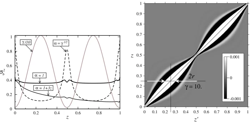
_{2 ð0:1;100Þ.}

This result is illustrated inFig. 1, where the left panel shows

r

2

bðzÞfor different functions

a

ðzÞ, while

c

ðzÞis defined as

follows:

c

ðz_{Þ ¼}0:2þ9:8ð1cosð4

p

z_ÞÞ: ð5:3Þ

The right panel shows the background error covariance matrix which looks identical for all functions

a

ðz_Þconsidered:

a

¼1,

a

¼1þ3z, and

a

¼p

c

ffiffiffi. It can be seen inFig. 1(left) that in the case

a

¼pffiffiffi

c

, which corresponds to constant value of weights

a

i=pffiffiffiffi

c

i in(5.1), the variance changes significantly with

c

ðzÞ. However, if

a

is constant (case

a

¼1), then the variance has a

nearly constant value, while the changes in the correlation radius are related mainly to

c

ðzÞ. Therefore, the Eq.(5.1)can be used to generate a family of covariances such that

a

ðz_Þand

c

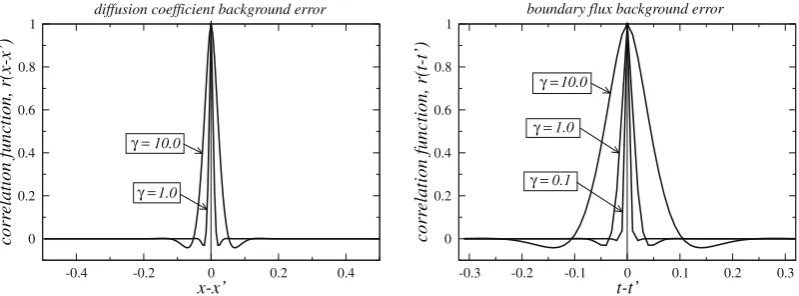
ðz_Þdefine mainly the variance and the correlation radius, respectively. Examples of the background error correlation functions, which correspond to different values of constant

c

for

a

¼1 are presented inFig. 2, for the diffusion coefficient estimation problem (left) and for the boundary flux estimation problem (right).

In the initial-value DA problem, the background function for the subsequent DA can be computed as an optimal solution (analysis) evolved to the instantt¼T, i.e. as

u

ðT;xÞ. Similarly, the background error covariance matrix could be computed as the evolved analysis error covariance matrix. This is possible in principle, though difficult to implement for large-scale prob-lems. For the boundary value estimation problem such a possibility does not generally exist. Therefore, the descriptions sim-ilar to(5.1)might be a reasonable choice to defineV1orVn1. Let us note that this is a typical approach for certain applications

(for example, for inverse heat transfer problems[1]).

5.2. Preconditioning the Hessian

In[6]we have reported the numerical algorithm for computing the covariance matrix with the use of the quasi-Newton BFGS method[4,16]for the case of the initial-value control problem. The same algorithm can be used in the case of param-eter estimation.

Let us consider the problem(2.3). We approximate the covariance operatorVdkby the inverse Hessian of the auxiliary DA

problem(3.24) and (3.25). The inverse Hessian (orH-covariance) is computed as a collateral result of the BFGS iterations in the course of solving the minimization problem(3.24) and (3.25). In order to obtainH1_{in the explicit form, the sequence of}

the BFGS updates must be applied to the unity vectors. For particular details of this approach we refer to[6].

0 0.2 0.4 0.6 0.8 1

z 0

0.2 0.4 0.6 0.8 1

σ

1/2

α= 1

γ/10

= 1+3z

α

α = γ

b 2

0 0.1 0.2 0.3 0.4 0.5 0.6 0.7 0.8 0.9 1

z'

0 0.1 0.2 0.3 0.4 0.5 0.6 0.7 0.8 0.9 1

z

-0.001 0 0.001

γ = 10.

[image:9.595.94.496.545.741.2]

2r

Fig. 1. Left - the background error variancer2

The process of building the inverse Hessian by the BFGS algorithm can be accelerated by using a preconditioning. Usually, a preconditioning is aimed to accelerate the convergence rate of a minimization procedure. However, this is a different task. For example, the minimization procedure may converge long before any sensible approximation of the inverse Hessian is built. Here we assume that the preconditioned Hessian would have much fewer eigenvalues remote from 1 and, therefore, require fewer quasi-Newton updates to be represented.

SinceHis self-adjoint, we must consider a preconditioned Hessian in a symmetric form, for example:

e H_{¼ ð}B1

ÞHB1

; ð5:4Þ

with some operatorB:Yp ! Yp. We can prove that the operatorHe is the Hessian of the following modified auxiliary DA

problem: finddkanddusuch that

@du @t F

0

uð

u

;k_Þd

u

_¼F0 kð

u

;kÞB

1_dk

; t_{2 ð}0;T_Þ;

d

u

_jt¼0¼0; S2ðdkÞ ¼inf

v₂Yp

S2ð

v

Þ; 8 > > < > > :

ð5:5Þ

where

S2ðdkÞ ¼1₂ðV1B1ðdkn1Þ;B1ðdkn1ÞÞYpþ 1

2ðV2ðCd

u

n2Þ;Cd

u

n2ÞYobs: ð5:6Þ

Therefore, one may use the BFGS algorithm to solve the minimization problem(5.5) and (5.6)and findðHe_Þ1_{. After that,}

hav-ingðHe_Þ1_{, one can easily recoverH}1 _{using the formula}

H1

¼B1

ðHe_Þ1

ðB1

Þ: ð5:7Þ

For the boundary flux estimation problem (Section4.3) the modified auxiliary problem(5.5) and (5.6)reads as follows: find du1;du2andd

u

such that

@du @t F

0

ð

u

Þd

u

¼0; t_{2 ð}0;T_Þ

d

u

jt¼0¼0;

k_ð

u

_Þ@du

@x jx¼0¼B11du1; kð

u

Þ@_@dxujx¼1¼B21du2; S2ðdu1;du2Þ ¼ inf

v₁;v₂

S2ð

v

₁;

v

₂Þ; 8 > > > > > < > > > > > :

ð5:8Þ

where

S2ðdu1;du2Þ ¼1₂X 2

i¼1

Vð₁iÞB1

i ðduini;1Þ;Bi1ðduini;1Þ

L2ð0;TÞþ 1

2ðV2ðCd

u

n2Þ;Cd

u

n2ÞYobs: ð5:9Þ

One can recoverH1 _{by the formula(5.7), whereBis 2}

2 block-diagonal matrix withB1andB2as blocks.

An important issue is how to construct the operatorB1_{. Usually one tries to takeB}1_{in such a way that the spectrum of}

the preconditioned HessianHe _{¼ ð}B1

ÞHB1_{is clustered around 1. This means that the majority of eigenvalues ofHe are equal}

or close to 1. Theoretically, the best choice of B1 _{is such that He is the identity operator. Thus, one should achieve} B1

ðB1

ÞH1_{orBBH. One possibility to constructB}1_{is to consider an approximationH}

aH. If we compute the

Chole-sky factorization forH1

a in the formH

1

a ¼LL, then we can takeB

1

¼L. Sometimes, it is beneficial to compute the Cholesky factorization forHaitself, i.e.Ha¼LL, then we can takeB1¼ ðLÞ1.

-0.4 -0.2 0 0.2 0.4

x-x’ 0 0.2 0.4 0.6 0.8 1 corr

elation function, r(x-x’) γ =

γ =

1.0 10.0

diffusion coefficient background error

-0.3 -0.2 -0.1 0 0.1 0.2 0.3

t-t’ 0 0.2 0.4 0.6 0.8 1 corr

elation function, r(t-t’)

γ = γ = γ = 0.1 1.0 10.0

[image:10.595.100.500.74.222.2]

boundary flux background error

Fig. 2.Scaled correlation function of the background error rðzz0_Þ for different constant c. Left – the diffusion coefficient estimation problem

In this paper we assume thatHa¼V1. This choice ofHacorresponds to the ‘first level’ preconditioning commonly used in

variational DA[3,5]. In the 1D case, the weight matrixV1defined by(5.1) and (5.2)is a five-diagonal banded matrix. For a

givenV1we compute the Cholesky factorizationV1¼LL, whereLis the lower triangular factor ofV1. Then, the productB1

v

(required in Eqs.5.5, 5.6 and 5.7) can be obtained by the backward substitution sweep involvingL_{, whileðB}1

Þ

v

(required in(5.7)) – by the forward substitution sweep involvingL. With this arrangement the matrixVn1 is never computed. Other

possible approaches to Hessian preconditioning are considered in[5,24,26]. Let us emphasize that the development of an efficient preconditioner would be the key implementation issue for the method proposed.

5.3. Additional implementation details

As a model for numerical implementation we consider the 1D convection–diffusion equation. We use the implicit time discretization as follows

u

i

u

i1

ht þ

@ðwui Þ

@x

@ @x kð

u

i Þ@

u

i

@x

¼0; i_{2 ð}1;. . .;mtÞ; x2 ð0;1Þ; ð5:10Þ

wherei_¼1;. . .;mt is the time integration index,ht¼T=mtis a time step. The spatial operator is discretized on a uniform

mesh (hx¼1=mxis the spatial discretization step,mx is the total number of mesh nodes) using the ‘power law’ first-order

scheme as described in[15].

When the boundary flux estimation problem is considered (Section4.3), the model equation is nonlinear (k_¼k_ð

u

Þ). In this case for each time step we perform nonlinear iterations, assuming initially thatk_ð

u

i_{Þ ¼kð}

_u

i1

Þ, and keep iterating until

(5.10) is satisfied (i.e. the norm of the left-hand side in(5.10) becomes smaller than a threshold

1¼1012pffiffiffiffiffiffimx). For the

parameter estimation problem (Section4.2) we assume that the diffusion coefficient does not depend on the solution

u,

but is a function ofx, i.e.k_¼k_ðx_Þ. Let us notice that even though the model equation becomes linear in this case, the param-eter estimation problem remains nonlinear (that can be seen from(4.15)).

Let us note that the auxiliary DA problem(3.24) and (3.25)includes the TLM of the original evolution problem. In order to solve the minimization problem(3.24) and (3.25)using the BFGS algorithm one also needs the adjoint model that computes the gradient of(3.25)with respect to the unknown parameters. Both in[6]and in the present paper we use the TLM and adjoint models generated by means of Automatic Differentiation (AD) [8]. The TLM and adjoint models produced in this way are known as consistent models. We stress that the use of consistent models is essential to obtain theH-covariance. However, if the TLM code is produced by means of AD, it could be difficult to separate manually the part of the code which computes the solution of the original evolution problem and the part which computes the solution of the TLM. With this arrangement the original nonlinear problem has to be solved as many times as the TLM whereas it should be solved only once. Let us notice that for solving the auxiliary problem(3.24) and (3.25)the consistency between the TLM and the adjoint models is all that is required. Therefore, the compromise approach would be: (a) derive analytically and separately imple-ment the TLM, and (b) generate the adjoint model by means of AD, using the TLM source code as the input for the AD engine. In numerical experiments, theH-covariance matrixVwill be compared with the ensemble covariance matrixVb, obtained

by the fully nonlinear ensemble method. This method is presented in detail in[6]. Here we would only mention that this method allows the covariance matrix to be estimated without any linearization involved, and therefore is considered for the verification purpose. The ensemble sizeM_¼400 is being used in all ensemble computations presented in this paper. This size has been chosen such that the sampling error is noticeably smaller (10%) than the optimal solution error.

6. Numerical results

We mentioned already that DA allows the uncertainty in model parameters/controls to be reduced. The background error covariance matrixVn1 (a priori covariance matrix) is a measure of uncertainty in model parameters before DA. The variance

r

2

bcan be considered as the original uncertainty magnitude. The (optimal solution error) covariance matrixVdk(a posteriori

covariance matrix) is a measure of uncertainty in the sought parameters after DA and the variance

r

2

dkis the uncertainty

magnitude after DA, respectively. Let us introduce the function

f_ðz_{Þ ¼}

r

2

ðz_Þ=

r

2

bðzÞ; z2 ½0;1; ð6:1Þ

where

r

2_{ðzÞis theH-variance. The functionfquantifies the ’usefulness’ of observation data in terms of reducing the original}

6.1. Distributed coefficient estimation

Here we refer to the diffusion parameter estimation problem stated in Section4.2. In this problem one tries to estimate the unknown diffusion coefficientk_ðx_Þ;x_{2 ð}0;1Þusing a set of incomplete observations of the field

u

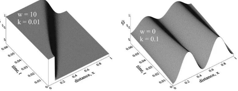
ðt;x_Þwhich evolves from the known initial stateu. Let us note that the evolution Eq.(4.11)is now linear, however the parameter estimation problem is always nonlinear. We consider two cases: the convection-dominated caseðw_¼10; k_¼0:01; Pe_¼w=k_¼103_{), and the}

pure diffusion caseðw¼0;k¼0:1Þ. In the first case the initial state is the step-function

u_¼ 1; x60:1

0; x>0:1

;

in the second case it is defined by the formula

u_¼0:5ð1þcos_ð4

p

x_ÞÞ: ð6:2Þ

The ‘true’ field

_u

_ðt;xÞfor both cases is presented inFig. 3(left) andFig. 3(right), respectively. In geophysics, the convection-dominated problems are usual in meteorology and surface-water applications. For example,Fig. 3(left) may represent a heat wave propagation. Even though the (eddy) diffusion could be relatively small, it is an important parameter that defines the front dissipation rate. The diffusion-dominated problems arise in groundwater[20]and oil-reservoir modelling.

In order to compute theH-covarianceVwe solve the modified auxiliary DA problem(5.5) and (5.6)withk¼kby the BFGS algorithm, then retrieve V_¼H1 _{using (5.7). The discretization parameters for the numerical model are: m}

x¼200, hx¼0:05; mt¼128; T¼0:064; ht¼0:005.

6.1.1. Convection-dominated evolution model

In this part we consider the observation scheme which consists of five sensors located in the middle of the computational domain at the pointsx_¼0:4;0:45;0:5;0:55;0:6; the observation error variance is constant inxwith

r

obs¼3104. Since

the diffusion coefficient is always positive, the function

a

ðx_Þ(which largely defines

r

bðxÞ) must be considered such that

3

r

bðxÞ<kðxÞ; 8x. We chose

a

ðxÞto satisfy the condition 3

r

bðxÞ kðxÞ. This allows us to apply the largest possible

back-ground errorn1, while keepingkb¼kþn1 positive (and therefore physically meaningful) in ensemble computations. This

is a limitation of the theory presented in this paper that results from the assumption of the Gaussian (i.e. symmetric) dis-tribution of the background error and could be particularly noticeable for small_kðxÞ.

In the first example we consider_{kðxÞ ¼0:01; w¼10;}

_c

_{ðxÞ ¼10, and}

_a

_{ðxÞ ¼410}4_{. The result obtained by the BFGS (the}

functionf_ðx_Þ,(6.1)) is presented inFig. 4(left) in bold solid line. One can see that the behaviour offis relatively simple and generally resembles the behaviour of the variance in the initial-value control problem ([6]). The minima offare located in the vicinity of sensors. Between the sensorsfgrows to a level which depends mainly on the background error correlation radius controlled by

c

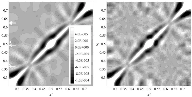
ðxÞ. Outside the domain covered by sensorsfgrows approaching 1, even though there is an interme-diate level off<1 in the upstream direction. For the same conditions we compute the ensemble^f(presented in the marked line). One can notice that^_{fis in a good agreement withfobtained by the BFGS, particularly within the area where sensors}

dominate the look off. TheH-covariance matrixVobtained by the BFGS and_V^ _{obtained by the ensemble method are}

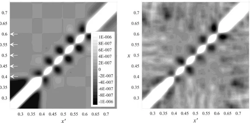
pre-sented inFig. 5(left) andFig. 5(right), respectively.

In order to compare cases with different k_ðx_Þwe consider the following functions:k_ðx_{Þ ¼}0:1; w_¼10;

c

ðx_{Þ ¼}10, and

a

ðxÞ ¼4102. The result obtained by the BFGS is presented inFig. 4(left) in faint solid line. We note that now the structure offis even simpler than before and that the largerk_ðx_Þcan be better estimated (with the same

r

obs).

[image:12.595.109.497.606.754.2]

In the second example presented inFig. 4(right) we comparefcomputed with

c

ðx_{Þ ¼}10 (in bold solid line) and with the variable

c

defined by(5.3)(in faint solid line). One can notice a very significant difference between these cases. This example underlines the crucial role of the background error correlation radius (controlled by

c) in computing the covariance.

6.1.2. Pure diffusion evolution model

In this part we refer toFig. 6(left). We consider two observation schemes. Each scheme consists of six sensors located in the middle of the spatial domain, however the sensors are located differently. In both cases the observation error variance is constant inxwith

r

obs¼5103. In the first case the sensors are evenly distributed (locations are shown by arrows marked a), the correspondingf_ðx_Þis presented in faint solid line. In the second case the sensors are put in pairs (locations are shown

0.3 0.4 0.5 0.6 0.7

x 0

0.2 0.4 0.6 0.8 1

ς

BFGS, k = 0.01 BFGS, k = 0.1 ENS., k = 0.01, M = 400

σ = , γ = obs 3.0E-4 10

w = 10 ,

0.3 0.4 0.5 0.6 0.7

x 0

0.2 0.4 0.6 0.8 1

ς

γ = 10

[image:13.595.102.490.77.222.2]

γ −Eq.(5.3)

[image:13.595.94.502.274.475.2]

Fig. 4.Left –fand^_{ffork¼0:01 andffork¼0:1. Right –ffor varyingcand for constantc¼10.}

Fig. 5.Diffusion coefficient estimation problem. Left –H-covariance. Right – ensemble covariance.

0 0.1 0.2 0.3 0.4 0.5

x 0

0.2 0.4 0.6 0.8 1

ς

BFGS, a - sensors BFGS, b - sensors ENS., M = 400 initial condition

a a a a

b bb

b w = 0, k = 0.1,σ = , γ = obs 5.0E-3 10

0.25 0.3 0.35 0.4 0.45 0.5 0.55 x

0 0.2 0.4 0.6 0.8 1

ς

initial condition

single

pair single

pair

a a

b b b b

[image:13.595.101.491.527.672.2]

by arrows markedb), the result is presented in bold solid line. We notice that in the second case the functionfðx_¼0:375Þis smaller by an order of magnitude than in the first case. For the second case we also present the ensemble^_{fby the marked}

line. One can see a very good agreement betweenfand^f, particularly in the area covered by sensors. For this case theH -covarianceVand the ensemble covarianceVb are presented inFig. 7(left) andFig. 7(right), respectively.

In the case of pure diffusion the behaviour offis more complex than in the convection-dominated case. This can be ex-plained by considering the expression(4.14), for example. We notice that the function@

u

_{=@x, which is responsible for} deliv-ering information from the sensors via the adjoint variable, is multiplied by@

u

=@x. Because of that, in the areas with small field gradients the gradient of the cost functionS0_{ðkÞis dominated by the background term. Due to the symmetric nature of} the diffusion process, the extremum points in the initial state do not change their original location (see e.g.Fig. 3(right)), i.e. the areas with small and big gradients remain at certain locations.

Below we refer toFig. 6(right). Let us assume that the observation system includes a single sensor and the initial condi-tion satisfies to(6.2). First we put the sensor at the locationx_¼0:5, where the field gradient tends to zero, but the field value

u

ðt;x_Þchanges most significantly. Next we put the sensor at the locationx_¼0:375, where the field gradient reaches its

max-imal value, however the field value remains constant

u

ðt;x_{Þ ¼}0:5. The results (functionfðx_Þ) are presented in bold solid and bold dashed lines, respectively. In the first case (x_¼0:5), as expected, no significant reduction infis achieved. In the second caseðx_¼0:375Þthe result is actually even worse (around the sensor location). The point is that the constant field value mea-sured by the sensor may correspond to any initial condition that satisfiesu_¼0:5ð1þcosð2npxÞÞ; n_¼2;3;. . ., which means

that without the background term the problem has no unique solution. This analysis leads to the conclusion that in given circumstances it might be beneficial to observe the field gradient, rather than the field value. In order to support this idea, instead of a single sensor atx¼0:375, we put a pair of sensors located closely (x1¼0:365 andx2¼0:385). The

correspond-ingfis presented inFig. 6(right) by a thin dashed line. One can see that we have achieved a drastic decrease inf. Finally, we put a pair of sensors (x1¼0:49 andx2¼0:51) instead of a single sensor atx¼0:5. One can see that the same decrease infis

not achieved. This must be expected since the field gradient atx_¼0:5 is equal to zero. A practical conclusion from these

numerical experiments is that at the areas where the field gradient is big enough one may use a pair of closely located sen-sors to catch the field gradient. In this case the quality of the diffusion coefficient estimation can be greatly improved. A sim-ple structure of fin the convection-dominated problem considered above can now be explained. The reason is that the convection moves the field pattern (front) across the domain, therefore a similar field and field gradient values are supplied to each sensor at some stage.

6.2. Boundary flux estimation problem

Here we refer to the parameter estimation problem stated in Section4.3. For a trivial initial conditionu¼0, one looks to estimate unknown boundary fluxesu1andu2using a set of incomplete observations

u

obs. The observation scheme includes

three sensors located at pointsx_¼0:2;0:5;0:8. The evolution Eq.(4.16)is nonlinear because the diffusion coefficientk_ð

u

Þ depends on

u. In order to set up tests we consider two cases of

k_ð

u

Þas shown inFig. 8(left).

The diffusion coefficientk_ð

u

Þvaries from the levelk1to the levelk2(k2>k1forcase Iandk2<k1forcase II) within the

interval½

u

0D;

u

0þDsubjected to the rule as follows:

[image:14.595.101.499.73.274.2]

k_ð

u

Þ ¼k1þ₂k2k1₂k2sinð

p

ð

u

u

0Þ=ð2DÞÞ: ð6:3Þ

We can control the degree of nonlinearity (up to a nearly discontinuousk_ð

u

Þ) by changing parametersDandk1;k2. Incase I

we choose

u

0¼0:3; k1¼0:05; k2¼1:0; D¼0:15, in case II-u0¼0:0; k1¼1:0; k2¼0:05; D¼0:1. The discretization

parameters for the numerical model are:mx¼200,hx¼0:05; mt¼64; T¼0:64; ht¼0:01. The ‘true value’ of the driving

boundary conditionu1for two cases under consideration are presented inFig. 8(right), whileu2¼0.

6.2.1. Inflow driving boundary

A distinguishing feature of this case is that the driving boundary at x¼0 is the inflow boundary (i.e.w>0ðjwj ¼2Þ), therefore the boundary perturbations propagate far enough into the domain. The field variable

_u

_ðx;t_Þfor this case is pre-sented inFig. 9(left), the diffusion coefficientk_ð

_u

_ðx;t_ÞÞ inFig. 9(right). We compute theH-covariance and the ensemble

-0.4 -0.2 0 0.2 0.4 0.6 0.8

ϕ 0

0.2 0.4 0.6 0.8 1

k

case II

∆ ∆

ϕ0

case I

k

k1

2

0 0.1 0.2 0.3 0.4 0.5 0.6

time, t -1

-0.5 0 0.5 1 1.5

boundary flux, x=0

[image:15.595.100.496.74.215.2]

case I case II

Fig. 8.Left – diffusion coefficientkðuÞ. Right – ‘true’ boundary conditions.

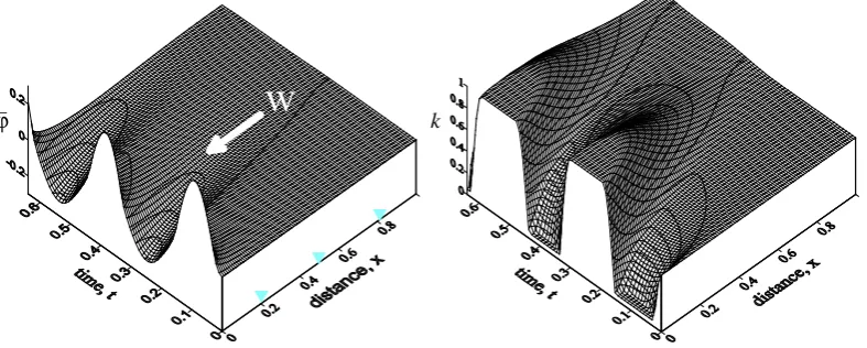
w

[image:15.595.104.491.392.553.2]

ϕ

_ k

Fig. 9.Left – ‘true’ fielduðt;xÞ. Right – diffusion coefficientkðuðt;xÞÞ.

0 0.1 0.2 0.3 0.4 0.5 0.6

time, t 0

0.1 0.2 0.3 0.4

variance

BFGS background ensemble, M = 400

x = 0, inflow

x = 1, outflow

10.0 _obs

α = , γ = , σ =

k - case I, w = 2.0, 1.0 3.0E-2

0 0.1 0.2 0.3 0.4 0.5 0.6

time, t 0

0.02 0.04 0.06 0.08 0.1

variance

k - case I, w = 2.0, α = , γ = , σ =4.0 10.0 obs 7.5E-3

[image:15.595.101.497.599.751.2]

covariance assuming the following properties of errorsni:

a

¼1:0;

c

¼10:0,

r

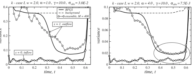
obs¼0:03. The corresponding variances are

presented inFig. 10(left).

The first thing to be noticed in this figure is that the variance of the unknown fluxu1at the inflow boundaryx¼0 (solid

line) is much smaller than the background variance (dashed line), which means it can be well identified almost everywhere, excluding a ‘blind spot’ intervalðTdt;T_Þ. The match between theH-variance and the ensemble variance is good. This result is trivial and could easily be predicted from a qualitative analysis.

An unexpected conclusion is however that the flux u2 at the outflow boundary x¼1 can also be partially identified

ðt_{2 ð}0:38;0:6ÞÞ. This ‘identifiable’ part of the boundary conditionu2corresponds to a larger value of the diffusion coefficient k_ð

u

Þ(Fig. 9(right)), which is due to the nonlinearity. This behaviour would be difficult to expect without computations.

Let us notice that the match between theH-variance and the ensemble variance foru2is not particularly good. Indeed, the H-covariance is an approximation of the actual covariance which relies on the linearized error evolution model (TLM). In ([6]) we emphasize that the tangent linear hypothesis is a local sufficient condition. Because of that, theH-covariance could be a good approximation of the covariance far beyond the validity of this condition. The accuracy of the linearization de-pends on two factors: a) degree of the nonlinearity; b) magnitude of errorsni. This means that the estimation/control

prob-lem could be extremely nonlinear, yet the linearization would be accurate if the magnitude of errors is sufficiently small. In the case considered above the magnitude of the background error was noticeably larger than the unknown fluxes themselves.

To illustrate this point we consider another case with the errors magnitude being 1/4 of those in the previous case:

a

¼4:0;

c

¼10:0;

r

obs¼0:0075. The variances for this case are presented inFig. 10(right). We can see that theH- and

the ensemble variances are now in a much better agreement, particularly in the area highlighted by the ellipse. Therefore, for smaller errors, theH-covariance is again a good approximation of the covariance.

Next we analyse how theH-covarianceVdepends on the correlation radius of the background errorr_ðtt0_{Þ, which is} con-trolled by

c

(Fig. 2(right)). The functionf¼fðt_Þfor different

c

is presented inFig. 11foru1(left) and foru2(right). In[6]we

mentioned that

c

is a crucial parameter which defines theH-covariance. The same conclusions can be drawn fromFig. 11. We

[image:16.595.110.494.411.560.2]

can see that for a weakly correlated background error

c

¼0:1, the functionfis close to 1 even for the inflow boundaryx_¼0,

Fig. 11(left). As

c

grows,fbecomes smaller, i.e. the efficiency of DA increases. This example shows that if we specify the back-ground error correlation radius wrongly (which may happen since

c

is often a priori defined function!), then the covariance

0.5 0.6

time, t 0

0.2 0.4 0.6 0.8 1

ς

γ =

γ =

γ =

0.1

1.0

10.0

x = 0, inflow boundary

0 0.1 0.2 0.3 0.4 0 0.1 0.2 0.3 0.4 0.5 0.6

time, t 0

0.2 0.4 0.6 0.8 1

ς

γ =

γ =

γ =

0.1

1.0

[image:16.595.106.500.596.754.2]

10.0 x = 1, outflow boundary

Fig. 11.Left –fat inflow boundaryx¼0 for differentc. Right –fat outflow boundaryx¼1.

w

ϕ_

k

estimate (bothH-covariance and the ensemble covariance) could be wrong. One could possibly state that any discussion on

the ‘linearization error issue’ is irrelevant unless we are certain about the background error correlation function.

0 0.1 0.2 0.3 0.4 0.5 0.6

time, t 0

0.1 0.2 0.3 0.4

variance

BFGS background ensemble, M = 400

x = 0, outflow

10.0

x = 1, inflow

[image:17.595.200.391.141.294.2]

3.0E-2 k - case II, w = -2.0, α = , γ = , σ = 1.0 obs

Fig. 13. Background, H- and ensemble variances.

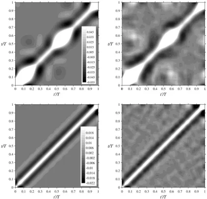
Fig. 14. Left, upper –H-covariance fordu1. Right, upper – ensemble covariance fordu1. Left, lower –H-covariance fordu2. Right, lower – ensemble

[image:17.595.84.507.337.743.2]

6.2.2. Outflow driving boundary

A distinguishing feature of this case is that the driving boundary atx_¼0 is the outflow boundary (i.e.w<0ðjw_{j ¼}2Þ), therefore perturbations at the boundary do not propagate far into the domain. The field variable

_u

_ðx;tÞfor this case is pre-sented inFig. 12(left), the diffusion coefficientk_ð

_u

_ðx;t_ÞÞ– inFig. 12(right).

We compute the H-covariance and the ensemble covariance assuming the following properties of errors ni:

a

¼1:0;

c

¼10:0;

r

obs¼0:03. The variances are presented inFig. 13. Once again, one can notice that the flux at inflow

boundaryx_¼1 can be well identified, which is a result one should expect. An unexpected result is that the fluxu1at outflow

boundaryx_¼0 can also be partly identified (because of the nonlinearity). Moreover, we know exactly which parts of the boundary (when) and how well this can be done. Therefore, in order to analyse numerically the degree of uncertainty reduc-tion in a model parameter (control), theH-covariance has to be computed. The similar theoretical analysis is often a difficult task, for the nonlinear case in particular.

TheH-covariance and the corresponding ensemble covariance matrices are presented inFig. 14, upper panel (for the out-flow boundary,x_¼0) and lower panel (for the inflow boundary,x_¼1). A satisfactory agreement between theH-covariance and the ensemble covariance in both cases can be noticed (as well as for the variances presented inFig. 13).

6.3. Benefits of preconditioning

The preconditioning technique is described in Section5.2. As a preconditioner we use the Cholesky factor of the weight matrixV1, which is inverse to the background error covariance matrixVn1. In[6]we reported that as the correlation radius of

the background error (controlled by

c) grows, the number of iterations required to form the inverse Hessian quickly

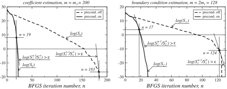
in-creases approaching the number of unknowns. This is true for the problems considered in this paper if the original auxiliary problem(3.24) and (3.25)or(4.20) and (4.21)is considered. However, if we solve the modified auxiliary DA problem for the preconditioned Hessian(5.5) and (5.6)or(5.8) and (5.9), the quasi-Newton approximation of the inverse Hessian requires much fewer BFGS updates to be formed. Examples of the convergence history with and without preconditioning (for other-wise equivalent conditions) are presented inFig. 15for the diffusion coefficient estimation problem (left), and for the bound-ary flux estimation problem (right). These two cases correspond to the problems considered earlier and presented in

Fig. 4(left) and inFig. 10(right), respectively.

The criteria used to stop the BFGS iterations takes into account the slope of the convergence curve

log S

n1

i Sn_i

!

>

; i_¼1;2; ð6:4Þ

wherenis the BFGS iteration number,Sn

i is the corresponding value of the cost functionalSi. The value of the threshold

used

in all examples was

¼4. In the vast majority of numerical tests this criterion leads to accurate results.

A major advantage of using the inverse BFGS update formula is that one can compute theH-covariance using the product

Hv, that is without the need to form and keep the matrixH. However, if the number of the BFGS iterations is large, this advantage would be quickly annihilated because of the need to keep a large number of updates (pair-vectors), and to run both the TLM and adjoint models at each iteration. The examples of the convergence history presented inFig. 15show that with an efficient preconditioning theH-covariance matrix can be computed in a number of iterations much less than the number of unknownsm, therefore much less memory is required to keep the updates. Let us recall that the direct method

for computing the covariance via the Hessian matrixH(sometimes referred to as the Fisher information matrix) would re-quire allmruns of the TLM plus the inversion of the matrixH.

0 50 100 150 200

BFGS iteration number, n -20

-10 0 10 20 30

precond. off precond. on

n = 19

n = 183

coefficient estimation, m = m = 200

log(S /S ) >ε 1 1 x

log(S )

2

log(S )

2 n-1 n

2

1

log(S /S ) >n-1 n ε

0 20 40 60 80 100 120

BFGS iteration number, n -30

-20 -10 0 10 20

precond. off precond. on

log(S )

n = 17

n = 124

boundary condition estimation, m = 2m = 128

log(S /S ) >

ε

2 ε

t

2

log(S )1

n n-1

n-1 n

log(S /S ) >

2

[image:18.595.107.490.74.224.2]

1 1