Estimating factor models for multivariate volatilities : an innovation expansion method

factor models for multivariate volatilities : an innovation expansion

method. In: Proceedings of COMPSTAT 2010. A Physica Verlag

Heidelberg product . Physica-Verlag HD, Heidelberg, pp. 305-314. ISBN

978-3-7908-2603-6 , http://dx.doi.org/10.1007/978-3-7908-2604-3_28

This version is available at

https://strathprints.strath.ac.uk/29324/

Strathprints is designed to allow users to access the research output of the University of Strathclyde. Unless otherwise explicitly stated on the manuscript, Copyright © and Moral Rights for the papers on this site are retained by the individual authors and/or other copyright owners. Please check the manuscript for details of any other licences that may have been applied. You may not engage in further distribution of the material for any profitmaking activities or any commercial gain. You may freely distribute both the url (https://strathprints.strath.ac.uk/) and the content of this paper for research or private study, educational, or not-for-profit purposes without prior permission or charge.

Any correspondence concerning this service should be sent to the Strathprints administrator:

[email protected]

The Strathprints institutional repository (https://strathprints.strath.ac.uk) is a digital archive of University of Strathclyde research outputs. It has been developed to disseminate open access research outputs, expose data about those outputs, and enable the

Estimating Factor Models for Multivariate

Volatilities:

An Innovation Expansion Method

Jiazhu Pan1

, Wolfgang Polonik2

, and Qiwei Yao3

1

Department of Mathematics and Statistics, University of Strathclyde

26 Richmond Street, Glasgow, G1 1XH, UK,[email protected]

2

Division of Statistics, University of California at Davis

Davis, CA 95616, USA,[email protected]

3

Department of Statistics, London School of Economics

London WC2A 2AE, UK,[email protected]

Abstract. We introduce an innovation expansion method for estimation of factor

models for conditional variance (volatility) of a multivariate time series. We estimate the factor loading space and the number of factors by a stepwise optimization algorithm on expanding the “white noise space”. Simulation and a real data example are given for illustration.

Keywords: dimension reduction, factor models, multivariate volatility.

1

Introduction

Factor modelling plays an important role in the analysis of high-dimensional multivariate time series( see Sargent and Sims, 1977; Geweke, 1977) because it is both flexible and parsimonious. Most of factor analysis in the literature is for the mean and conditional mean of a multivariate time series and panel data, see Pan and Yao (2008) and a series of papers of article by Forni, Hallin, Lippi and Reichlin (2000,2004), and Hallin and Liˇska (2007).

For the conditional variance, which is so-called volatility, the multivariate generalized autoregressive conditional heteroskedastic (GARCH) models are commonly used, see Engle and Kroner (1995), Engle (2002), Engle & Shep-pard (2001). But a multivariate GARCH model often has too many parame-ters so that it is difficult to estimate the model, which is a high-dimensional optimization problem. Factor models for volatility are useful tools to over-come the overparametrisation problem, e.g. Factor-ARCH (Engle, Ng and Rothschild 1990).

2

Models and methodology

Let{Yt}be ad×1 time series, andE(Yt|Ft−1) = 0, whereFt=σ(Yt, Yt−1,· · ·).

Assume thatE(YtYtτ) exists, and we use the notationΣy(t) =var(Yt|Ft−1).

Pan et al. (2009) consider a common factor model

Yt=AXt+εt, (1)

whereXtis ar×1 time series,r < dis unknown,Ais ad×runknown constant

matrix, {εt} is a sequence of i.i.d. innovations with mean 0 and covariance

matrix Σε, and εt is independent of Xt and Ft−1. This assumes that the

volatility dynamics of Y is determined effectively by a lower dimensional volatility dynamics ofXtplus the static variation ofεt, as

Σy(t) =AΣx(t)Aτ+Σε, (2)

where Σx(t) =var(Xt|Ft−1). The component variables ofXt are called the

factors. There is no loss of generality in assuming rk(A) = r and requiring the column vectors of A = (a1,· · · , ar) to be orthonormal, i.e. AτA = Ir,

whereIr denotes ther×ridentity matrix.

We are concerned with the estimation for the factor loading spaceM(A), which is uniquely defined by the model, rather than the matrixAitself. This is equivalent to the estimation for orthogonal complement M(B), where B

is ad×(d−r) matrix for which (A, B) forms ad×dorthogonal matrix, i.e.

Bτ_{A= 0 andB}τ_B=I

d−r. Now it follows from (1) that

BτYt=Bτεt. (3)

Hence Bτ_Y

tare homoscedastic components since

E{BτYtYtτB|Ft−1}=E{BτεtεtτB}=E{BτYtYtτB}=Bτvar(Yt)B.

This implies that

BτE[{YtYtτ−var(Yt)}I(Yt−k∈C)]B= 0, (4)

for anyt, k≥1 and any measurableC⊂Rd_.

For matrixH = (hij), let ||H|| ={tr(HτH)}1/2 denote its norm. Then

(4) implies that

k0

X

k=1

X

C∈B

w(C)¯

¯ ¯ ¯

n

X

t=k0+1

E[Bτ{YtYtτ−var(Yt)}BI(Yt−k ∈C)]

¯ ¯ ¯ ¯

2

= 0 (5)

where k0 ≥ 1 is a prescribed integer, B is a finite or countable collection

of measurable sets, and the weight function w(·) ensures the sum on the right-hand side finite. In fact we may assume that P

Factor Models for Multivariate Volatility 3

(n−k0)−1P_k0<t≤nYtYtτ. This is due to the fact Bτvar(Yt)B = BτΣεB,

and

(n−k0)−1

n

X

t=k0+1

BτYtYtτB = (n−k0)−1

n

X

t=k0+1

BτεtετtB

a.s.

→ BτΣεB,

see (3). ThereforeBτ_Σˆ

yB is a consistent estimator forBτvar(Yt)B for allt.

Denote

Dk(C) = (n−k0)−1

n

X

t=k0+1

(YtYtτ−Σˆy)I(Yt−k ∈C).

Now (5) suggests to estimateB≡(b1,· · · , bd−r) by minimizing

Φn(B) =

k0

X

k=1

X

C∈B

w(C)¯

¯ ¯

¯BτDk(C)B

¯ ¯ ¯ ¯ 2 (6) = k0 X k=1 X

1≤i,j≤d−r

X

C∈B

w(C)©

bτiDk(C)bjª

2

subject to the conditionBτ_B=I

d−r. This is a high-dimensional optimization

problem. Further it does not explicitly address the issue how to determine the number of factors r. We present an algorithm which expands the inno-vation space step by step and which also takes care of these two concerns. Note for any bτ_{A= 0, Z}

t≡bτYt(=bτεt) is a sequence of independent

ran-dom variables, and therefore, exhibits no conditional heterosedasticity. The determination of theris based on the likelihood ratio test for the null hypoth-esis that the conditional variance of Ztgiven its lagged valued is a constant

against the alternative that it follows a GARCH(1,1) model with normal innovations. See also Remark 1(vii) below.

Put

Ψ(b) =

k0

X

k=1

X

C∈B

w(C)[bτDk(C)b]2,

Ψm(b) =

k0

X

k=1

n

2

m−1

X

i=1

X

C∈B

w(C)[ˆbτiDk(C)b]2+

X

C∈B

w(C)[bτDk(C)b]2

o

.

An Innovation Expansion Algorithm for estimating B and r: let pbe

an integer between 1 and k0 and α∈ (0,1) specify the level of significance

test.

Step 1. Compute ˆb1which minimisesΨ(b) subject to the constraintbτb=

1. LetZt= ˆbτ1Yt. Compute the 2log-likelihood ratio test statistic

T = (n−k0)

©

1+log¡ 1

n−k0

n

X

t=k0+1

Z2 t ¢ª −min n X

t=k0+1

©Z

2

t

σ2

t

+log(σ2

t)

ª

,

where σ2

t = α+βZt2−1+γσ 2

t−1, and the minimisation is taken

over α > 0, β, γ ≥ 0 and β+γ < 1. Terminate the algorithm

with ˆr=dand ˆB= 0 ifT is greater than the topα-point of the

χ2

2-distribution. Otherwise proceed to Step 2.

Step 2. Form= 2,· · ·, d, compute ˆbmwhich minimizesΨm(b) subject to

the constraint

bτ_{b= 1, b}τ_ˆb

i= 0 fori= 1,· · ·, m−1. (8)

Terminate the algorithm with ˆr=d−m+1 and ˆB = (ˆb1,· · ·,ˆbm−1)

ifT, calculated as in (7) but withZt=|ˆbτmYt|now, is greater than

the topα-point of theχ2

2-distribution.

Step 3. In the event thatTp never exceeds the critical value for all 1 ≤

m≤d, letr= 0 and ˆB=Id.

Remark 1. (i) The algorithm grows the dimension ofM(B) by 1 each time

until a newly selected direction ˆbmbeing relevant to the volatility dynamics

ofYt. This effectively reduces the number of the factors in model (1) as much

as possible without losing significant information.

(ii) The minimization problem in Step 2 is a d-dimensional subject to constraint (8). It has only (d−m+ 1) free variables. In fact, the vector b

satisfying (8) is of the form

b=Amu, (9)

whereuis any (d−m+ 1)×1 unit vector,Amis ad×(d−m+ 1) matrix with

the columns being the (d−m+ 1) unit eigenvectors, corresponding to the (d−m+1)-fold eigenvalue 1, of matrixId−BmBmτ, andBm= (ˆb1,· · ·,ˆbm−1).

Note that the other (m−1) eigenvalues ofId−BmBmτ are all 0.

(iii) We may let ˆA consist of the ˆr (orthogonal) unit eigenvectors, corre-sponding to the common eigenvalue 1, of matrixId−BˆBˆτ (i.e. ˆA=Ad−rˆ+1).

Note that ˆAτ_Aˆ=I

ˆ

r.

(iv) A general formald×1 unit vector is of the formbτ _{= (b}

1,· · · , bd),

where

b1=

d−1

Y

j=1

cosθj, bi= sinθi−1

d−1

Y

j=i

cosθj (i= 2,· · ·, d−1), bd= sinθd−1,

whereθ1,· · ·, θd−1 are (d−1) free parameters.

(v) We may chooseBconsisting of the balls centered at the origin inRd_.

Note thatEYt−k = 0. When the underlying distribution ofYt−k is symmetric

and unimodal, such aBis the collection of the minimum volume sets of the distribution ofYt−k, and thisBdetermines the distribution ofYt−k (Polonik

1997). In numerical implementation we simply usew(C) = 1/K, whereK is the number the balls inB.

(vi) Under the additional condition that

cτ_A{E(X

Factor Models for Multivariate Volatility 5

if and only ifAτ_{c= 0, (4) is equivalent to}

E{(bτiYtYtτbi−1)I(Yt−k∈C)}= 0, 1≤i≤d−r, k≥1 andC∈ B.

See model (1). In this case, we may simply useΨ(·) instead ofΨm(·) in Step

2 above. Note that forb satisfying constraint (8), (9) implies

Ψ(b) =

k0

X

k=1

X

C∈B

w(C)¡

uτAτmDk(C)Amu¢

2

. (11)

Condition (10) means that all the linear combinations ofAXtare genuinely

(conditionally) heteroscadastic.

(vii) When the number of factors r is given, we may skip all the test steps, and stop the algorithm after obtaining ˆb1,· · · ,ˆbr from solving the r

optimization problems.

Remark 2. The estimation of A leads to a dynamic model for Σy(t) as

follow:

ˆ

Σy(t) = ˆAΣˆz(t) ˆAτ+ ˆAAˆτΣˆyBˆBˆτ+ ˆBBˆτΣˆy,

where ˆΣy = n−1P1≤t≤nYtYtτ, and ˆΣz(t) is obtained by fitting the data

{Aˆτ_Y

t, 1 ≤ t ≤ n} with, for example, the dynamic correlation model of

Engle (2002).

3

Consistency of the estimator

Forr < d, letHbe the set consisting of alld×(d−r) matrices H satisfying

the conditionHτ_H=I

d−r. ForH1, H2∈ H, define

D(H1, H2) =||(Id−H1H1τ)H2||={d−r−tr(H1H1τH2H2τ)}

1/2

. (12)

Denote our estimator by ˆB=argminB∈H_DΦn(B).

Theorem 1. Let C denote the class of closed convex sets in Rd_.

Un-der some mild assumptions (see Pan et al. (2009)), if the collection B is a countable subclass ofC, thenD( ˆB, B0)

P

→0.

4

Numerical properties

We always set k0 = 30, α = 5%, and the weight function C(·)≡ 1. Let B

4.1 Simulated examples

Consider model (1) withr= 3 factors, andd×3 matrixAwith (1,0,0),(0,0.5,0.866) (0,−0.866,0.5) as its first 3 rows, and (0,0,0) as all the other (d−3) rows. We consider 3 different settings for Xt = (Xt1, Xt2, Xt3)τ, namely, two sets

of GARCH(1,1) factorsXti=σtietiandσti2 =αi+βiXt2−1,i+γiσ2t−1,i, where

(αi, βi, γi), fori= 1,2,3, are

(1, 0.45, 0.45), (0.9, 0.425, 0.425), (1.1, 0.4, 0.4), (13)

or

(1, 0.1, 0.8), (0.9, 0.15, 0.7), (1.1, 0.2, 0.6), (14)

and one mixing setting with two ARCH(2) factors and one stochastic volatil-ity factor:

Xt1=σt1et1, σ2_t1= 1 + 0.6X 2

t−1,1+ 0.3X 2

t−2,1, (15)

Xt2=σt2et2, σ2t2= 0.9 + 0.5X 2

t−1,2+ 0.35X 2

t−2,2,

Xt3= exp(ht/2)et3, ht= 0.22 + 0.7ht−1+ut.

We let {εti}, {eti} and {ut} be sequences of independent N(0,1) random

variables. Note that the (unconditional) variance of Xti, for eachi, remains

unchanged under the above three different settings. We set the sample size

n= 300,600 or 1000. For each setting we repeat simulation 500 times.

Table 1.Relative frequency estimates ofrwithd= 5 and normal innovations

ˆ

r

Factors n 0 1 2 3 4 5

GARCH(1,1) with 300 .000 .046 .266.666.014 .008

coefficients (13) 600 .000 .002 .022.926.032 .018

1000 .000 .000 .000.950.004 .001

GARCH(1,1) with 300 .272 .236 .270.200.022 .004

coefficients (14) 600 .004 .118 .312.500.018 .012

1000 .006 .022 .174.778.014 .006

Mixture (15) 300 .002 .030 .166.772.026 .004

600 .000 .001 .022.928.034 .014

1000 .000 .000 .000.942.046 .012

We conducted the simulation withd= 5,10,20. To measure the difference betweenM(A) andM( ˆA), we define

D(A,Aˆ) ={|(Id−AAτ) ˆA|1+|AAτBˆ|1}/d2, (16)

Factor Models for Multivariate Volatility 7

0.0 0.2 0.4 0.6 0.8

n=300 n=600 factors (4.1)

n=1000 n=300 n=600 factors (4.2)

n=1000 n=300 n=600 factors (4.3)

n=1000

Errors of estimation for factor space

Fig. 1. Boxplots of D(A,Aˆ) with two sets of GARCH(1,1) factors specified,

re-spectively, by (13) and (14), and mixing factors (15). Innovations are Gaussian and

d= 5.

0.2 0.4 0.6 0.8

n=300 n=600 d=10, factors (4.1)

n=1000 n=300 n=600 d=20, factors (4.1)

n=1000 n=300 n=600 d=10, factors (4.2)

n=1000 n=300 n=600 d=20, factors (4.2)

n=1000 Errors of estimation for factor space

Fig. 2.Boxplots ofD(A,Aˆ) with two sets of GARCH(1,1) factors specified in (13)

and (14), normal innovations andd= 10 or 20.

We report the results withd= 5 first. Table 1 lists for the relative fre-quency estimates forrin the 500 replications. When sample sizenincreases, the relative frequency for ˆr= 3 (i.e. the true value) also increases. Even for

n = 600, the estimation is already very accurate for GARCH(1,1) factors (13) and mixing factors (14), less so for the persistent GARCH(1,1) factors (14). For n = 300, the relative frequencies for ˆr = 2 were non-negligible, indicating the tendency of underestimating ofr, although this tendency dis-appears when n increases to 600 or 1000. Figure 1 displays the boxplots of

D(A,Aˆ). The estimation was pretty accurate with GARCH factors (13) and mixing factors (15), especially with correctly estimatedr. Note withn= 600 or 1000, those outliers (lying above the range connected by dashed lines) typically correspond to the estimates ˆr6= 3.

Table 2. Relative frequency estimates of r with GARCH(1,1) factors,

normal innovations andd=10 or 20

ˆ

r

Coefficients d n 0 1 2 3 4 5 6 ≥7

(13) 10 300 .002 .048 .226.674.014 .001 .004 .022

10 600 .000 .000 .022.876.016 .012 .022 .052

10 1000 .000 .000 .004.876.024 .022 .022 .052

20 300 .000 .040 .196.626.012 .008 .010 .138

20 600 .000 .000 .012.808.012 .001 .018 .149

20 1000 .000 .000 .000.776.024 .012 .008 .180

(14) 10 300 .198 .212 .280.248.016 .008 .014 .015

10 600 .032 .110 .292.464.018 .026 .012 .046

10 1000 .006 .032 .128.726.032 .020 .016 .040

20 300 .166 .266 .222.244.012 .004 .001 .107

20 600 .022 .092 .220.472.001 .001 .012 .180

20 1000 .006 .016 .092.666.018 .016 .014 .172

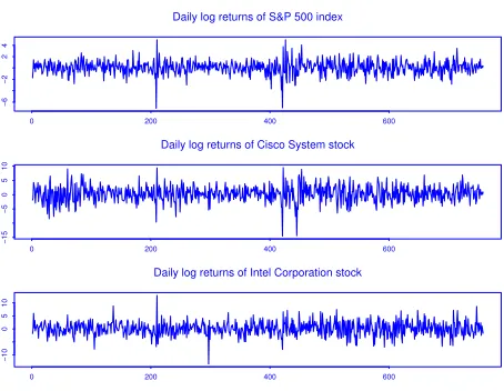
Daily log returns of S&P 500 index

0 200 400 600

−6

−2

2

4

Daily log returns of Cisco System stock

0 200 400 600

−15

−5

0

5

10

Daily log returns of Intel Corporation stock

0 200 400 600

−10

0

5

10

Fig. 3. Time plots of the daily log-returns of S&P 500 index, Cisco System and

Intel Coprporation stock prices.

accurate whennincreases, and the estimation with the persistent factors (14) is less accurate than that with (13).

4.2 A real data example

Factor Models for Multivariate Volatility 9

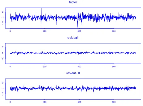
factor

0 200 400 600

−10

0

10

residual I

0 200 400 600

−10

0

10

residual II

0 200 400 600

−10

0

10

Fig. 4.Time plots of the estimated factor and two homoscedastic compoments for

the S&P 500, Cisco and Intel data.

Lag

ACF

0 5 10 15 20 25

0.0

0.2

0.4

0.6

0.8

1.0

ACF of squared factor

Lag

ACF

0 5 10 15 20 25

0.0

0.2

0.4

0.6

0.8

1.0

ACF of absolute factor

Fig. 5.The correlograms of squared and absulote factor for the the S&P 500, Cisco

and Intel data

is ˆr = 1 with ˆAτ _{= (0.310, 0.687, 0.658). The time plots of the estimated}

factorZt≡AˆτYtand the two homoscedastic components ˆBτYtare displayed

in Figure 4. TheP-value of the Gaussian-GARCH(1,1) based likelihood ratio test for the null hypothesis of the constant conditional variance for Zt is

0.000. The correlograms of the squared and the absolute factor are depicted in Figure 5 which indicates the existence of heteroscedasticity in Zt. The

fitted GARCH(1,1) model forZtis ˆσ2t = 2.5874 + 0.1416Z

2

t−1+ 0.6509ˆσ 2

t−1.

In contrast, Figure 6 shows that there is little autocorrelation in squared or absolute components of ˆBτ_Y

t. The estimated constant covariance matrix is

ˆ

Σ0=

 

1.594 0.070 4.142

−1.008−0.561 4.885

 .

Series 1

ACF

0 5 10 15 20 25

0.0 0.2 0.4 0.6 0.8 1.0

Series 1 and Series 2

0 5 10 15 20 25

0.0

0.1

0.2

0.3

0.4

Series 2 and Series 1

Lag

ACF

−25 −20 −15 −10 −5 0

0.0 0.1 0.2 0.3 0.4 Series 2 Lag 0 5 10 15 20 25

0.0 0.2 0.4 0.6 0.8 1.0

ACF of squared residuals

Series 1

ACF

0 5 10 15 20 25

0.0 0.2 0.4 0.6 0.8 1.0

Series 1 and Series 2

0 5 10 15 20 25

0.0

0.1

0.2

0.3

Series 2 and Series 1

Lag

ACF

−25 −20 −15 −10 −5 0

0.0 0.1 0.2 0.3 Series 2 Lag 0 5 10 15 20 25

0.0 0.2 0.4 0.6 0.8 1.0

ACF of absolute residuals

Fig. 6. The correlograms of squared and absulote homoscedastic compoments for

the the S&P 500, Cisco and Intel data

References

ENGLE, R. F. (2002): Dynamic conditional correlation a simple class of

multivari-ate GARCH models.Journal of Business and Economic Statistics, 20, 339350.

ENGLE, R. F. and KRONER, K.F. (1995): Multivariate simultaneous generalised

ARCH.Econometric Theory, 11, 122-150.

ENGLE, R. F., NG, V. K. and ROTHSCHILD, M. (1990): Asset pricing with a factor ARCH covariance structure: empirical estimates for Treasury bills.

Journal of Econometrics, 45, 213-238.

FORNI, M., HALLIN, M., LIPPI, M. and REICHIN, L. (2000): The generalized

dynamic factor model: Identification and estimation.Review of Economics and

Statistics,82, 540-554.

FORNI, M., HALLIN, M. LIPPI, M. and REICHIN, L. (2004): The generalized

dynamic factor model: Consistency and rates. Journal of Econometrics,119,

231-255.

GEWEKE, J. (1977): The dynamic factor analysis of economic time series. In:

D.J. Aigner and A.S. Goldberger (eds.):Latent Variables in Socio-Economic

Models, Amsterdam: North-Holland, 365383.

HALLIN, M. and LIˇSKA, R. (2007): Determining the number of factors in the

general dynamic factor model.Journal of the American Statistical Association,

102, 603-617.

LIN, W.-L. (1992): Alternative estimators for factor GARCH models – a Monte

Carlo comparison.Journal of Applied Econometrics, 7, 259-279.

PAN, J., POLONIK,W., YAO,Q., and ZIEGELMANN,F. (2009): Modelling

multi-variate volatilities by common factors.Research Report, Department of

Statis-tics, London School of Economics.

PAN, J. and YAO, Q. (2008). Modelling multiple time series via common factors.

Biometrika_{, 95, 365-379.}

SARGENT,T. J. and SIMS, C.A. (1977): Business cycle modelling without

pre-tending to have too much a priori economic theory. In: C. A. Sims (ed.):New

Methods in Business Cycle Research, Minneapolis: Federal Reserve Bank of