Longevity-indexed annuities

      

City, University of London Institutional Repository

Citation

:

Denuit, M., Haberman, S. and Renshaw, A. E. (2011). Longevity-indexed annuities. North American Actuarial Journal, 15(1), pp. 97-111. doi:

10.1080/10920277.2011.10597611

This is the accepted version of the paper.

This version of the publication may differ from the final published

version.

Permanent repository link:

http://openaccess.city.ac.uk/4036/

Link to published version

:

http://dx.doi.org/10.1080/10920277.2011.10597611

Copyright and reuse:

City Research Online aims to make research

outputs of City, University of London available to a wider audience.

Copyright and Moral Rights remain with the author(s) and/or copyright

holders. URLs from City Research Online may be freely distributed and

linked to.

City Research Online: http://openaccess.city.ac.uk/ [email protected]

LONGEVITY-INDEXED LIFE ANNUITIES

Abstract.

This paper addresses the problem of the sharing of longevity risk between an annuity provider and a group of annuitants. An appropriate longevity index is designed in order to adapt the amount of the periodic payments in life annuity contracts. This accounts for unexpected longevity improvements experienced by a given reference population. The approach described in the present paper is in contrast with Group Self-Annuitization where annuitants bear their own risk. Here, the annuitants only bear the non-diversifiable risk that the future mortality trend departs from that of the reference forecast. In that respect, the life annuities discussed in this paper are substitutes for reinsurance and securitization of longevity risk.

Key words and phrases.

Longevity risk, mortality projection, Lee-Carter model.

1. Introduction and motivation

In this paper, we address the problem of the sharing of longevity risk between an annuity provider and a group of annuitants. A conventional approach to this problem is via reinsurance. However, reinsurance treaties covering longevity risk are usually expensive and many life insurance companies are reluctant to buy long-term reinsurance coverage (e.g. because of credit risk).

Securitization offers an interesting alternative to reinsurance; see, e.g., Denuit, Devolder & Goderniaux (2007) and the references therein. In that respect, the first publicly offered longevity derivative was issued by the European Investment Bank (EIB) together with BNP in November 2004. This was a 25-year bond, issued by EIB, with coupon payments linked to the mortality experience of the base group of males in England and Wales who were age 65 in 2003 (precisely, to the proportions of this cohort reaching ages 66 and over). The initial coupon was scaled each year by the survival rate of the base population group. To actuaries this is simply a group life annuity on the base population. In this paper, we further investigate this idea for annuities but no longer in the context of securitization. Rather, we scale the annuity payments in a similar way.

their study. This can be understood as follows. The number of survivors is still large at these ages and even modest improvements compared to the life table which is used for pricing and reserving result in large additional costs for the annuity provider. This clearly shows that annuity providers need financial instruments with a maturity of over 15-20 years in order to offset the longevity risk. This horizon may be too distant for many investors so that securitization for longevity risk may be difficult to implement in practice.

Considering the cost of these risk management tools, a viable alternative might well be to leave the systematic part of the mortality risk with the annuitants. Indeed, when the insurance company contracts long-term obligations, it is often efficient to let the premium evolve according to some well-chosen index. This creates an effective risk sharing mechanism between the insurance company and the policyholders, leaving the latter with the risk reflected in the index (often, inflation or some other systematic risk that cannot be diversified across the portfolio). Since immediate life annuities are sold for a single premium, it is not possible to let the amount of premium depend on an appropriate index, but it would be possible to adjust the insurer's payments: if the actual longevity exceeds that of a reference forecast, then the payments are reduced accordingly. We acknowledge that the coverage against individual longevity risk provided by such a product is inferior to that of a life annuity offering guaranteed payments. However, transferring only part of the longevity risk to the annuity provider decreases its need for risk capital, reinsurance and/or securitization and is expected to make the product less expensive for future retirees. For a given amount of premium, the policyholders will be granted a higher initial periodic payment in a longevity-indexed life annuity. Annuitants have then to decide whether they prefer fixed periodic payments or agree to let them vary according to some specified longevity index. Note also that, in the case where the actual mortality improvements turn out to be weaker than expected, the payments to the annuitants are increased correspondingly in a longevity indexed contract. Moreover, periodic payments can be subjected to caps and floors in order to reduce the adverse effect of longevity improvements on annuity payments. For instance, the contract could specify that, in any case, the annuity payments will not be smaller than 80%, say, of the initial amount, whatever the improvements in longevity.

The idea of indexing life insurance products is of course not new. It is common in actuarial practice to let the premiums and/or benefits depend on the development of mortality. However, in the context of life annuities used to provide an income after retirement, the individual is poorly placed to absorb the longevity risk in the post-retirement phase. In this respect, insurance companies have provided in recent years more flexible products including a significant investment element. For instance, premiums are converted into units of an investment fund or insurance benefits are linked to some public stock index. Hence, policyholders buying these products agree to support (part of) the investment risk compared to classical policies offering guaranteed interest rate. The volatility implied by these increasingly popular new products is much higher than that implied by the longevity indexed annuities discussed in the present paper. Therefore, investors favouring insurance products offered without guaranteed interest rates could also consider buying longevity indexed products as long as they offer comparable returns. Increased returns are made possible since, as noted above, passing part of the longevity risk to the annuitants substantially decreases the insurer's need for capital or for reinsurance.

pool together and form a fund in order to provide for protection against longevity. These Authors report that annuities where payments reflect evolving mortality have for some time been issued in the US by the Teachers’ Insurance and Annuity Association (TIAA) and that, historically, the impact of annual mortality adjustments has been relatively modest. Compared with GSA, the type of annuities discussed in the present paper is not a tontine scheme and offers a superior protection to policyholders. The annuitants only bear the systematic part of the longevity risk, whereas the insurer covers the random fluctuation of mortality as well as the expected future mortality improvements and possible departures from the guaranteed interest rates. In the framework of Piggott, Valdez & Detzel (2005), Van de Ven & Weale (2008) discuss the way in which payments from pooled annuity funds need to be adjusted when future mortality rates are not known with certainty. They investigate “mortality adjusted” annuities in which aggregate mortality risk is transferred from the provider to the annuitants, allowing for the level of risk aversion of the annuitant.

The approach described in the present paper shares some similarities with the “adaptive algorithmic annuities” designed by Luthy et al. (2001). These Authors suggest the use of frequent estimates of the actual mortality in order to adjust the benefits to the policyholders. More precisely, forecasts of future mortality are updated and produce new expected present values of life annuity payments. The benefits paid to the annuitants are then scaled according to these new amounts of premium. Compared to this approach, the updates of periodic payments proposed in the present paper are based on official data published by National Institute of Statistics or regulatory authorities (and not on mortality forecasts). This makes the indexing mechanism more transparent to policyholders.

Richter & Weber (2009) also discuss annuity contracts with benefits linked to actual mortality experience, including an actuarial model for calculating and reserving. These authors discuss whether and to what extent such products are also advantageous for policyholders compared to conventional annuity products. The proposal made by Richter & Weber (2009) shares some similarities with the product designed in this paper but is closer to the GSA philosophy. Also, it relies on a new best-estimate for future mortality each time the annuity payment is updated, as in Luthy et al. (2001).

The present paper is organized as follows. Section 2 describes indexed life annuity products. Section 3 studies these insurance contracts when the Lee-Carter model is used to describe the trend in future mortality. In Section 4, we limit the revision of the annuity payment, to protect annuitants. Section 5 offers numerical illustrations. The final Section 6 concludes and discusses the results. Some points are deferred to an appendix, to avoid distracting the reader with technicalities.

To end with, let us introduce some notation used throughout this paper. Henceforth, we analyze the changes in mortality as a function of both age x and calendar time t. This is the so-called age-period approach. The remaining lifetime of an individual aged x on January the first of year t is denoted as T_x(t). Thus, this individual will die at age x+T_x(t)in calendar

year t+T_x(t). Then, q_x(t)=P

[

T_x(t)≤1

]

is the probability that an x-aged individual in

2. Longevity indexed life annuities

Let us consider an individual buying an immediate longevity indexed life annuity at age x in ₀

calendar year t . According to this contract, the annuitant receives an annual payment as long ₀

as he or she survives. The amount specified in the contract is one monetary unit, scaled by a longevity index.

Let p ₀ (t0 k)

ref k

x + + , k=0,K,

ω

−x0, be a forecast for the survival of some reference population to which the individual belongs, where

ω

denotes the ultimate age (for which the one-year survival probability vanishes). This forecast may be provided by governmental agencies performing mortality projections (National Institute of Statistics or insurance regulators). The reference population may be the general population of a given country or some market life table.

As time passes, the observed values of the one-year survival probabilities become available. In an indexed life annuity contract, the risk remaining with the annuitants is the spread between the forecast ( ₀ )

0 t k

pref_{x +k} + and its actual value (₀ )

0 t k

pobs_{x +k} + . Specifically, the annual payment due at time k is adjusted by the factor

∏

−

= +

+

+ ₊

+ =

= 1

0 0

0

0 0

) (

) (

) (

) (

0 0

0 0

0

k

j obs

j x ref

j x obs

x k

ref x k k t

j t p

j t p

t p

t p i

Hence, if the contract specifies an annual payment of 1, the annuitant receives a stream of payments _{, ,}K

2 1 ₀

0+ t +

t i

i as long as he or she survives.

Seen from t , this index is of course a random variable as the future survival probabilities are 0 unknown (but their distribution function can be derived from the mortality projection model). Hence, it becomes

) (

) (

0 0

0 0

0

t P

t p I

x k

ref x k k

t + = (2.1)

where (₀)

0 t

P_x

k is the future unknown survival probability from age x to age 0 x0 +k. The distribution of the random variable kPx₀(t0) can be derived from the mortality projection model used to forecast future longevity. In this paper, we concentrate on the Lee-Carter model but the approach nevertheless applies to any other model.

3. Distribution of the conditional expected present value of longevity indexed life annuity payments in the Lee-Carter model

3.1. Lee-Carter model

We recall the basic features of the classical Lee-Carter approach. In this framework, the population central death rate at age x in calendar year t, denoted asm t_x

( )

, is of the form

( )

lnm t_x =

α

_x+

β κ

_{x t}. (3.1) Interpretation of the parameters involved in model (3.1) is straightforward. The value of

α

_x is an average of lnm t over time t so that exp_x( )

α

_x represents the general shape of the age-specific mortality profile. The actual forces of mortality change over time according to an overall mortality index

κ

_t which is modulated by an age response variable

β

_x. The coefficient

β

_x indicates the sensitivity of different ages to the time trend so that the shape of the

β

_x profile indicates which rates decline rapidly and which slowly over time in response to changes in

κ

_t.

An appropriate error structure has to be specified in order to estimate the parameters involved in (3.1). Lee & Carter (1992) opted for Normal disturbances and an estimation procedure based on Singular Value Decomposition, i.e.

xt t x x x t

mˆ ( )=

α

+

β

κ

+

ε

ln

where mˆ t_x( ) is the observed death rate at age x in calendar year t and the error terms

ε

_xt are independent and Normally distributed with zero mean and constant variance. Binomial, Poisson or Negative Binomial regression models can also be used to estimate the parameters entering the decomposition (3.1). For more details about inference issues, we refer the interested reader to Pitacco et al. (2009).

In order to make forecasts, Lee & Carter (1992) assume that the

α

_x and

β

_x remain constant over time and forecast future values of

κ

_t using a standard univariate time series model. In the majority of studies based on the Lee-Carter mortality projection model, a simple random walk with drift, or ARIMA(0,1,0) model, is used to describe the dynamics of the time index

t

κ

; see, e.g., Denuit, Haberman & Renshaw (2010). In some cases, higher-order ARIMA models are needed to appropriately describe the time index. We retain the ARIMA(0,1,0) assumption in the text and we defer to the appendix the study of the general ARIMA(p,1,q) case. Henceforth, we assume that

t t

t

κ

θ

ξ

κ

= ₋1+ +

3.2. Conditonal survival probabilities in the Lee-Carter model

Let us denote as _dP t_x( |₀

κκκκ

) the random d-year survival probability for an individual aged x in year t , that is, the conditional probability that this individual reaches age x + d in year ₀ t₀ +d,

given the vector κκκκ of the κ_t. It is formally defined as

[

T t >d

κ

]

=

P x(0) dP tx( |0 κκκκ)

(

0

)

1

0

exp exp

d

x j x j t j j

−

+ + +

=

 

= − + 



∑

α

β κ

.

Let us define

(

0

)

( )

1 1

0 0

exp exp

d d

d x j x j t j j j

j j

S

α

β κ

δ

Z

− −

+ + +

= =

=

∑

+ =

∑

,

where δ_j =exp

( )

α_{x j+} >0 and

0

j x j t j

Z =β κ_{+ +} . Clearly _dP t_x( |₀ κκκκ) =exp(−S_d). Conditional on

0

t

κ , it follows that Z_j is Normally distributed with mean ( )

0 θ

κ β

µ_j = _{x+j t} + j and variance 2

2 2

) (

β

σ

σ

_j = _x+j j subject to the convention that a Normally distributed random variable with zero variance is constantly equal to its mean. Note that the mean and variance are taken conditionally on past values of the time index.

3.3. Life annuity conditional expected present value

Let us consider a basic life annuity contract paying 1 unit of currency at the end of each year, as long as the annuitant survives. The random life annuity single premium, that is, the conditional expectation of the payments made to an annuitant aged x in the year t given the ₀

time index, is

 

∑

∑

−

= =

=    

   

= 0 0 0 ₀

0

1 0 )

(

1

0 ) (0, ) ( ) (0, )

(

x

k x k t

T

k

x t E v k P t v k

a

x ω

κ

κ

κ

where v(.,.) is the deterministic discount factor (precisely, ( , )v s t is the present value at time s of a unit payment made at time t). Note that a tx( | )0

κκκκ

corresponds to the generation aged x in calendar year t , and accounts for future mortality improvements experienced by this 0

particular cohort. Clearly, a tx( | )0

κκκκ

is a random variable that depends on the future trajectory of the time index (that is, on

0, 0 1, 0 2,...

t t+ t+

κ κ

κ

). It can be seen as the systematic risk per contract in a sufficiently large portfolio. An analytical computation of the distribution function of a t_x( | )₀

κκκκ

seems to be out of reach.

For a longevity indexed contract, the annuity periodic payments are no longer constantly equal to 1 but become I_{t +k}

0 given in (2.1). In the Lee-Carter model, It0+k depends on

κ

and

(

( )

)

exp ) ( 0 0

0

κ

k

κ

ref x k k t k

t I p S

I ₊ = ₊ =

so that the conditional present value of the payments under a longevity indexed contract is

(

)

∑

∑

− = − = + = − 0 0 0 0 1 1 ) , 0 ( ) , 0 ( ) ( exp ) ( x k ref x k x k k k

t S v k p v k

I

ω ω

κ

κ

.

Thus, we see that the annuity provider is no longer subject to longevity risk when annuity payments are scaled by It₀+k: all of the systematic longevity risk is passed to the annuitants

and the provider is allowed to operate as if the reference life table exactly applies. In Section 4, we introduce caps and floors on I_{t +k}

0 in order to limit the impact of indexing.

3.4. Comonotonic approximations

Assuming a random walk with drift model for the

κ

_t’s, Denuit & Dhaene (2007) have proposed comonotonic approximations for the quantiles of the random survival probabilities

0 ( |

dP tx

κκκκ

). Since the expression for a tx( | )0

κκκκ

involves the weighted sum of the dP tx( |0

κκκκ

)’s, Denuit (2007, 2008) supplemented this first comonotonic approximation with a second one. Denuit, Haberman & Renshaw (2010) have extended these results to general ARIMA dynamics for the

κ

t’s. Here, we show that a similar idea applies to the longevity-indexed life

annuities.

Approximating S by a sum of perfectly dependent random variables, with the same marginal _d

distributions, gives the approximation

1

exp( ), with ~ (0,1)

d u

d d j j j

j o

S S

δ

µ σ

Z Z N

− =

≈ =

_∑

+ .

Since S is a sum of comonotonic random variables, its quantile function is additive. The _du

quantile function 1

u d

S

F− of u d

S is given by

(

)

1

1 1

0

( ) exp ( )

u d

d

j j j

S

j

F z

δ

µ σ

z

−

− −

=

=

∑

+ Φ , (3.2)

where Φ−1 is the quantile function of the standard Normal distribution.

Another approximation of S_d is l

[

|

]

d d d

S =E S Λ , where Λ_d is taken as the first-order

approximation of S , that is, _d 1

0 exp( )

d

d _j

δ

j

µ

j Zj

− =

Λ =

_∑

. A straightforward computation gives

1

2 2

0

1

exp ( ) (1 ( ( )) 2

d l

d j j j j j j

j

S r d Z r d

− =

 

=  + + − 

 

where ( ), r d_i i=0,1,...,d−1, is the correlation coefficient between Λ_d and Z , that is _i

{ }

{ }

∑

∑

∑

− = + + − = − = + + + = 1 0 2 1 0 1 0 2 , min ) exp( , min ) exp( ) ( d k k x j x k j k j d j i d j j x i x j j i k j j i d r

σ

β

β

µ

µ

δ

δ

σ

σ

β

β

µ

δ

. (3.3)

In the applications we have in mind, β_{x i+} and β_{x j+} typically have the same sign so that all of the r ’s are non-negative. This means that the _i S ’s are sums of comonotonic random _dl

variables and allows us to take advantage of the property of quantile additivity. Specifically, the quantile function of S is given by dl

1

1 1 2 2

0

1

( ) exp ( ) ( ) (1 ( ( )) 2

l d

d

j j j j j j

S

j

F z

δ

µ

r d

σ

z r d

σ

−

− −

=

 

=  + Φ + − 

 

∑

. (3.4)

From the approximations S_du and S derived for _dl S , we get the following approximations for _d

the random survival probabilities

0 ( |

dP tx κκκκ)

(

)

1

exp u(1 )

d

S

F− U

≈ − − and _dP t_x( |₀ κκκκ)

(

1

)

exp l (1 )

d

S

F− U

≈ − −

where U is uniformly distributed on the interval (0,1). Note that the same random variable U is used for all of the values of d, making the approximations to the conditional survival probabilities comonotonic. Hence, we obtain the following approximations for a t_x( | )₀ κκκκ

0 ( | )

x

a t κκκκ

(

1

)

1

exp u (1 ) (0, )

d

S d

F− U v d

≥ ≈

_∑

− − and 0 ( | ) x

a t κκκκ

(

1

)

1

exp l (1 ) (0, )

d

S d

F− U v d

≥

≈

_∑

− − .

Since these approximations are sums of comonotonic random variables, their quantile functions are additive. We then obtain the following approximations for the quantile function

0

1 ( | )

x

a t

F− _κκκκ of a t_x( | )₀ κκκκ

0

1 ( | )( )

x

a t

F− _κκκκ z

(

1

)

1

exp u (1 ) (0, )

d

S d

F− z v d

≥

≈

∑

− −

(3.5) where u1

d

S

F− is given in (3.2), and

0

1 ( | )( )

x

a t

F− _κκκκ z

(

1

)

1

exp l (1 ) (0, )

d

S d

F− z v d

≥

≈

∑

− −

where l1 d

S

F− is given in (3.4).

These approximations can be used to derive closed-form formulas for the quantiles of the present value of future annuity payments in the longevity indexed contract, as shown in the next section.

4. Caps and floors

The concept underlying longevity indexed life annuities is essentially a profit share: the insurer absorbs risk and profit from interest rates and idiosyncratic mortality risk, and the annuitants share with the insurer the pooled systematic longevity risk.

If the annuitants absorb all of the systematic risk, annuity payments may become arbitrarily low in old ages in the case of adverse experience. This situation appears to be highly undesirable given that longevity insurance is the main purpose of annuities. One could think of using safe side estimates of longevity risk, so that the expected outcome is an increase in old ages. However, past experience shows that safe side forecasts of longevity have often been exceeded and this approach may make the contract very expensive (or at least as expensive as traditional annuities).

A more efficient design would be to limit the systematic longevity risk passed to the annuitants, as discussed next.

As the annuitant is unlikely to be in a position to absorb all of the longevity risk, it seems reasonable to limit the impact of the index on the annuity payments. Therefore, instead of using the longevity index i , only part of it impacts on the annuity payment. For instance, if at t

most 20% of variation is allowed, then max

{

min

{

,1.2

}

,0.8

}

0 k

t

i ₊ is used to scale the annuity payment. This means that the index i_{t +k}

0 is replaced with its capped version

{

}

{

max min

}

max

min, ) maxmin , , (

0

0 i i i i i

i_{t +k} = _{t +k}

(4.1) for some 0<imin <1<imax.

Let (_min, _max)

0 i i

I_{t +k} be the index applying to the annuity periodic payments, that is,

{

}

{

max min

}

max

min, ) maxmin , , (

0

0 i i I i i

It +k = t +k

where It₀+k is given in (2.1). After k years, its realization is just it₀+k(imin,imax) defined in (4.1). The random variable ax₀(t0,imin,imax

κ

) is the corresponding conditional expectation if

the payments are subject to the index (_min, _max)

0 i i

I_{t +k} , k=1,2,…, that is,

 

   

   

=

∑

= +

κ

κ

) (

1

max min max

min 0

0 0

0

0( , , ) ( , ) (0, )

t T

k k t x

x

k v i i I E i

The comparison of a tx( | )0

κκκκ

with ax₀(t0,imin,imax

κ

) helps to quantify the risk passed from the annuity provider to the annuitant. Thus, ax₀(t0,imin,imax

κ

) is the systematic risk remaining

with the annuity provider.

Now, in the Lee-Carter model, (_min, _max)

0 i i

I_{t +k} depends on κ and is given by

(

)

{

}

{

max min

}

max min max

min, ) ( , ) maxmin exp ( ), ,

(

0 0

0 i i I i i p S i i

I_t+k = _t+k

κ

= _{k x}ref _k

κ

so that

(

)

∑

− = + − = 0 0 0 1 max min max min

0, , ) ( , )exp ( ) (0, )

( x k k k t

x t i i I i i S v k

a

ω

κ

κ

κ

Let us now consider the longevity indexed annuities. It is easily seen that each term included in the sum over k defining (₀,_min,_max )

0 t i i

κ

a_x in the Lee-Carter framework is non-increasing in

) (κ

k

S so that natural approximations are

( )

{

}

{

min exp , ,

}

exp

( )

(0, ) max ) , , ( 0 0 0 1 min max max min

0 i i p S i i S v k

t

a _ku

x k u k ref x k

x ≈

∑

−

− = ω

κ

(4.2) and

( )

{

}

{

min exp , ,

}

exp

( )

(0, ) max ) , , ( 0 0 0 1 min max max min

0 i i p S i i S v k

t

a kl

x k l k ref x k

x ≈

∑

−

− =

ω

κ

(4.3) These approximations turn out to be comonotonic sums so that their quantile functions are additive. Hence, the quantile functions of ax₀(t0,imin,imax

κ

) can be approximated as

(

)

{

}

{

min exp (1 ), ,

} (

exp (1 )

)

(0, )

max ) ( 1 1 min max 1 1 ) , , ( 0 0 max min 0 0 k v F i i F p F u k u k x S x k S ref x k i i t

a

ε

ε

ε

ω

κ ≈ − − − −

− = − −

_∑

and

(

)

{

}

{

min exp (1 ), ,

} (

exp (1 )

)

(0, )

max ) ( 1 1 min max 1 1 ) , , ( 0 0 max min 0 0 k v F i i F p F l k l k x S x k S ref x k i i t

a

ε

ε

ε

ω

κ ≈ − − − −

− =

−

−

_∑

5. Numerical illustrations

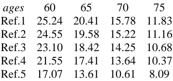
an ARIMA(0,1,0) for the dynamics for the time index. The reference life tables are as follows:

Ref.1 the point-wise projection (on a cohort basis) obtained for the England & Wales 1983-2004 male insured pensioners data set, using a Lee-Carter model, is taken as the reference life table. In this case, the reference forecast relates to the insurance market and not to the general population, and corresponds to the population being simulated, thereby reducing the “basis risk”. This particular choice of reference life table results in the vertical alignment that is visible for each agex in Fig 1. 0

Ref.2 the point-wise projection (on a cohort basis) obtained for the England & Wales male 1961-2005 general population using the Age-Period-Cohort version of the Lee-Carter model (as in Renshaw and Haberman (2006)) with ARIMA

(

0,1,0

)

dynamics is used as the reference life table in Fig 2.

Ref.3 the point-wise projection (on a cohort basis) obtained for the England & Wales male 1961-2005 general population using the standard Lee-Carter model with

(

0,1,0

)

ARIMA dynamics is used as the reference life table in Fig 3.

Ref.4 the CMI Bureau Life Office Pensioners current period standard life table (for male lives who have retired at normal retirement age – ultimate experience) is used as the reference distribution in Fig 4.

Ref.5 the empirical periodic life table obtained by averaging the England & Wales male 1961-2005 general population experience over time for each age (that is, the term

( )

exp

α

_x when fitting the conventional Lee-Carter model) is used as the reference life table in Fig 5.

The ultimate age

ω

, with one-year survival probability p t_ω( )=0, is set as ω =120 for all 5 reference life tables. The details of the construction of Refs.2-3 for the cohort years

0

2005−x and also the method used to “top-out” 4 of the 5 reference life tables (Refs.1-3, 5) is available from the Authors.

[image:12.595.208.387.598.682.2]

The next table displays the life expectancies at the given ages for the different reference life tables:

ages 60 65 70 75 Ref.1 25.24 20.41 15.78 11.83 Ref.2 24.55 19.58 15.22 11.16 Ref.3 23.10 18.42 14.25 10.68 Ref.4 21.55 17.41 13.64 10.37 Ref.5 17.07 13.61 10.61 8.09

Figures 1-5 depict the results. For each age x0 =60, 65, 70, 75, and each reference distribution, 2.5, 5, 50, 95, 97.5 u-type quantiles (4.2) and l-type quantiles (4.3) are displayed for the longevity indexed life annuities together with (3.5)-(3.6) where there is no indexing. In the figures, the values of (i_min,i_max) are given to make visible the effect of indexing. Here, (1,1) corresponds to no indexing and (0, +∞) corresponds to using actual mortality experience and so the confidence intervals shrink to a point. Thus, the effect of imin decreasing and

max

i increasing is to cause the intervals to become smaller. Note that in the (1,1) case, we are in the case considered by Denuit, Haberman & Renshaw (2010).

The more dispersed the quantiles, the more risk is retained by the annuity provider and the more expensive the indexed life annuity product. Discussing the attractiveness of the longevity indexed annuity contract is rather difficult, as it depends on the amount of premium charged by the insurance company for the different types of contracts and of the annuitant’s risk appetite. Nevertheless, the following discussion suggests that a good compromise could be found, offsetting most of the systematic longevity risk while limiting the impact of the indexing to an acceptable range.

We comment in more detail on the results as follows:

- Setting the bounds to be (1,1) means that the reference distribution does not feature in the calculations and there is no indexation. This reproduces the results in Denuit, Haberman & Renshaw (2010).

- In all of the cases, the intervals decrease in width as the bounds are increased. If we allow for more indexing then the width of the prediction intervals for the conditional expected present values of the annuity decreases as less risk is borne by the insurance company providing the longevity indexed annuity.

- Using Ref.1, the vertical alignment is a natural consequence of using the model predictions for the reference distribution.

- For the other 4 reference distributions, the predictions are in decreasing order of longevity (as measured by life expectancy) with increasing bounds (with one exception), indicating the effect of indexation. This effect does not appear to depend on whether or not the reference distribution was constructed on a period or cohort basis. The medians (and other quantiles) also react to the choice of the reference life table: thus, if the longevity expressed by the reference life table is smaller compared to the point forecast of the mortality projection model, then the index is more likely to be less than 1 and future annuity payments will probably be reduced.

- Also note that, where there is “basis risk” between the population and the reference distribution, the prediction intervals shift to the left as we move down the page (and the bounds widen). This is especially noticeable in Figure 5 which has the reference distribution with the lowest life expectancy. This effect is least noticeable in Figure 1 (as noted above) where there is a close match between the reference distribution and the distribution being simulated.

- In many cases, we see that allowing for +/-20% in the annuity payments greatly reduces the risk borne by the annuity provider.

mind that the model risk has not been accounted for in the computations so that the views expressed here may be too optimistic. We come back to this point in the final discussion.

6. Discussion

Life annuities will certainly become an essential product in the future, as our Western societies are progressively ageing. Actuaries have to make these products more attractive than they are today. The present paper makes some concrete proposals in that direction.

As an alternative to securitization, we have examined indexed life annuities, where periodic payments are scaled by the ratio of the proportion of the population still alive compared to some reference forecast. The systematic risk is thus passed to the annuitants. Considering the difficulties that have been experienced in issuing longevity-based financial instruments, this might well be an efficient alternative to help insurers to write annuity business.

As recalled in the introduction to this paper, it is usually considered that middle range longevity is the key risk to the insurer. The extreme old age systematic risk can be retained by the insurer, as it concerns a few policyholders and has thus limited financial impact. Fixing the annuity amount from some advanced age can be part of the design. This amounts to split the life annuity into a temporary annuity, subject to longevity indexing, and a fixed advanced-life delayed annuity (ALDA) in the terminology of Milevsky (2005).

Note that the idea of indexing also applies to ALDA. Under this deferred life annuity contract, the deferment period can be seen as a deductible: the policyholder finances his consumption until some advanced age, 80, 85 or even 90, say, and the insurer starts paying the annuity at this age provided the annuitant is still alive. Hence, the ALDA transforms the consumer choice and asset-allocation problem from a stochastic date of death to a deterministic one in which the terminal horizon becomes the annuity payment commencement date. If the index is publicly available then the annuitant is able to adjust his or her consumption level during the deferred period. Note that we could also think of alternative indexing mechanisms for ALDA. Considering a deferred life annuity bought at age 65 with payments starting at age 80, say, we could let the starting age vary according to actual longevity improvements: if longevity increases more than expected, then payments start at age 82 instead of 80, for instance.

In this paper, interest rates have been assumed to be deterministic (so that the v(0,k)s also are). If the interest rates were allowed to be stochastic, then conditional independence given κ needs to be postulated. This conditional independence may be justified by the fact that interest rates are influenced by the age pyramid of the population but not by the mortality itself. However, we note that Hanewald (2009) has found significant correlations between the Lee-Carter time index and real GDP growth rates and with unemployment rate changes in several OECD countries.

Acknowledgements

The Authors would like to thank an anonymous Referee for helpful comments that helped to improve the paper.

References

Denuit, M. (2007). Distribution of the random future life expectancies in log-bilinear mortality projection models. Lifetime Data Analysis 13, 381-397.

Denuit, M. (2008). Comonotonic approximations to quantiles of life annuity conditional expected present values. Insurance: Mathematics and Economics 42, 831-838.

Denuit, M. (2009). Dynamic life tables: construction and applications. Keynote Lecture. International Association of Actuaries Life Colloquium. Munich, Germany.

Denuit, M., Devolder, P., & Goderniaux, A.-C. (2007). Securitization of longevity risk: Pricing survivor bonds with Wang transform in the Lee-Carter framework. Journal of Risk and Insurance 74, 87-113.

Denuit, M., & Dhaene, J. (2007). Comonotonic bounds on the survival probabilities in the Lee-Carter model for mortality projections. Computational and Applied Mathematics 203, 169-176.

Denuit, M., Haberman, S., & Renshaw, A. (2010). Comonotonic approximations to quantiles of life annuity conditional expected present values: extensions to general ARIMA models and comparison with the bootstrap. ASTIN Bulletin 40, 331-349.

Hanewald, K. (2009). Mortality modeling: Lee-Carter and the macroeconomy. SFB 649 Discussion Paper 2009-008 (available at http://ssrn.com).

Khalaf-Allah, M., Haberman, S., & Verrall, R. (2006). Measuring the effect of mortality improvements on the cost of annuities. Insurance: Mathematics and Economics 39, 231-249.

Lee, R.D. & Carter, L. (1992). Modelling and forecasting the time series of US mortality. Journal of the American Statistical Association 87, 659-671.

Luthy, H., Keller, P.L., Binswangen, K., & Gmur, B. (2001). Adaptive algorithmic annuities. Bulletin of the Swiss Association of Actuaries, 123-138.

Milevsky, M. (2005). Real longevity insurance with a deductible: Introduction to advanced-life delayed annuities. North American Actuarial Journal 9, 109-122.

Piggott, J., Valdez, E., & Detzel, B. (2005). The simple analytics of a pooled annuity fund. Journal of Risk and Insurance 72, 497-520.

Renshaw, A. & Haberman, S. (2006). A cohort-based extension to the Lee-Carter model for mortality reduction factors. Insurance: Mathematics and Economics 38, 556-570.

Richter, A., & Weber, F. (2009). Mortality-indexed annuities: Managing longevity risk via product design. Discussion Paper 2009-14, Munich School of Management.

Valdez, E., Piggott, J., & Wang, L. (2006). Demand and adverse selection in a pooled annuity fund. Insurance: Mathematics and Economics 39, 251-266.

Van de Ven, J., & Weale, M. (2008). Risk and mortality-adjusted annuities. National Institute of Economics and social Research, Discussion Paper No 322.

Appendix

Here, we assume that the

κ

_t obey an ARIMA(p,1,q) model, with arbitrary values of p and q, which are to be determined. Furthermore, we assume that the

κ

_t are positively dependent, in the sense that the covariance between any pair ( , )

2

1 t

t κ

κ of time indices is non-negative. Since the κ_t are multivariate Normal, this ensures that the κ_t are positively associated, that is, the inequality

(

1 2

) (

1 2

)

1 t, t ,..., tn , 2 t, t ,..., tn 0

Cov_Ψ κ κ κ Ψ κ κ κ _≥

is valid for all values t₁< < <t₂ ... t_n and for all choices of the non-decreasing functions Ψ₁

and Ψ₂ such that the covariance exists.

In general, conditional on

0

t

κ , we still have that Z_j ~N(

µ σ

_j, 2_j) with moments

( )

0 0

2 2

and

j x jE t j j x j Var t j

µ ₌β _{+ }κ ₊ _ σ ₌ β ₊ _κ ₊ _

that can be computed according to the ARIMA specification retained.

The correlation coefficient between Λd and Z , ( ), i r di i=0,1,...,d −1, is given by

0 0

0 0

1 0

1 1

0 0

exp( ) [ , ]

[ , ] ( )

exp( ) [ , ]

d

d

j j x i x j t i t j

j i d

i _{d d}

i

i _{j k} j k j k x i x j t i t j

Cov Cov Z

r d

Cov

δ µ β β κ κ

σ σ _{σ δ δ µ µ β β κ κ}

−

+ + + +

=

− −

Λ _{+ + + +}

= =

Λ

= =

+

∑

∑ ∑