Model Switching and Model Averaging in
Time-Varying Parameter Regression Models
Miguel Belmonte
University of Strathclyde
Gary Koop
University of Strathclyde
January 2013, revised June 2014
Abstract: This paper investigates the usefulness of switching Gaussian state space models as a tool for implementing dynamic model selecting (DMS) or averaging (DMA) in time-varying parameter regression models. DMS methods allow for model switching, where a di¤erent model can be chosen at each point in time. Thus, they allow for the explanatory variables in the time-varying parameter regression model to change over time. DMA will carry out model averaging in a time-varying manner. We compare our exact method for implementing DMA/DMS to a popular existing procedure which relies on the use of forgetting factor approximations. In an application, we use DMS to select di¤erent predictors in an in‡ation forecasting application. We …nd strong evidence of model switching. We also compare di¤erent ways of implementing DMA/DMS and …nd forgetting factor approaches and approaches based on the switching Gaussian state space model to lead to similar results.
Keywords: Model switching, forecast combination, switching state space model, in-‡ation forecasting
1
Introduction
Bayesian model averaging or model selection (BMA or BMS) methods are commonly used when the researcher is faced with many models. See, for instance, Hoeting, Madi-gan, Raftery and Volinsky (1999) and Chipman, George and McCulloch (2001) for surveys of these methods. Numerous empirical applications use these methods. However, they were developed for regression models or other models where parameters are constant over time. In time series econometrics, motivated by strong empirical evidence of structural breaks or other forms of parameter change in many economic variables, models where parameters change over time have long been used. Models such as the time-varying parameter (TVP) regression model have enjoyed great popularity, particularly in macro-economics [see, among many others, Cogley and Sargent (2005), Cogley, Morozov and Sargent (2005), Primiceri (2005), Koop, Leon-Gonzalez and Strachan (2009), D’Agostino, Gambetti and Giannone (2011) and Korobilis (2013)]. Just as with constant coe¢ cient models, it is possible that the researcher working with TVP regression models will want to do model averaging and selection. However, it will typically be desirable to do these in a time varying manner. This leads to an interest in dynamic model averaging (DMA) or dynamic model selection (DMS). With DMA, the weights used in the model averag-ing procedure can change over time. With DMS, the model selected can change over time. This distinguishes it from conventional model selection methods where one model is selected and assumed to hold at all points in time.
The literature on DMA or DMS is much more limited than that on BMA or BMS. Perhaps the most prominent DMA approach for use with TVP regression models is that of Raftery, Karny and Ettler (2010). To explain what this algorithm involves, we begin by de…ning the set of models under consideration. Letytbe a dependent variable andZtbe a row vector containing explanatory variables. We have K models which are characterized by having di¤erent subsets of Zt as explanatory variables. Denoting these by Z
(k)
t for
k = 1; ::; K, a set of TVP regression models can be written as:
yt = Z
(k)
t
(k)
t +"
(k)
t (1)
(k)
t+1 = (k)
t +
(k)
t ;
"t(k) isN 0; "2(k) and (tk) isN 0;
(k)
.1
1Note that we have written the error variances, 2(k)
" and (k), as being constant. In empirical work
DMA and DMS can be done by calculating Pr (st=kjyt 1) for k = 1; ::; K where
st 2 f1;2; ::; Kg denotes which model applies at each time period and ys = (y1; ::; ys)0. DMS involves selecting, for forecasting yt given information available at time t 1, the single model with the highest value for Pr (st =kjyt 1). DMA involves averaging across models using these probabilities. Di¤erent approaches to DMA or DMS arise when dif-ferent models or methods are used to calculate Pr (st =kjyt 1). Raftery et al (2010), working in an application involving many potential explanatory variables and, hence, a large model space, uses forgetting factor methods to approximate Pr (st=kjyt 1). This leads to a computationally simple algorithm which does not require the use of Markov chain Monte Carlo (MCMC) methods. In applications with many potential explanatory variables [e.g. Raftery et al (2010), Koop and Korobilis (2012) and Koop and Tole (2013)], the algorithm of Raftery et al (2010) does seem to be the only computationally feasible algorithm currently available. However, as discussed in Section 3 of Raftery et al (2010), it is an approximate method that does not arise from a particular statistical model of model switching. Furthermore, it is a …ltering algorithm as opposed to a smoothing al-gorithm. That is, it provides the user with Pr (st=kjyt 1) for t = 1; ::; T as opposed to
Pr st =kjyT .
The purpose of this paper is to investigate the use of an alternative, model-based, way of allowing for time-varying model switching and compare it to the algorithm of Raftery et al (2010). This alternative is the family of switching Gaussian state space models described in, among other places, Kim (1994), Kim and Nelson (1999) and Fruhwirth-Schnatter (2001a, b). Switching Gaussian state space models will be described in the following section. Here we note only that they have been occasionally used in econometric applications [see Chapter 13 of Fruhwirth-Schnatter (2006) for a list of applications], but typically for state space models where the system matrices vary across regimes, not for selecting explanatory variables in TVP regression models [an exception being Chan et al (2012)]. An advantage of the use of switching Gaussian state space models is that results are not approximate, being based on a valid Bayesian posterior distribution. A further advantage is that either …ltered or smoothed estimates can be obtained using existing algorithms.
using switching Gaussian state space models in a setting with a small model space, it will raise concerns about the use of Raftery et al (2010)’s algorithm in the large model spaces where it is typically used. However, if the two approaches yield similar results, it will increase our con…dence in the use of the algorithm of Raftery et al (2010) in large model spaces.
This paper contains an application involving selecting between or averaging di¤erent independently produced forecasts of a dependent variable. That is, Zt will contain vari-ous forecasts of the dependent variable yt. Methods for combining forecasts provided by di¤erent models goes back to Bates and Granger (1969) and Granger (2006) provides a recent survey. Recent approaches related to our own include Guidolin and Timmermann (2009), which uses a Markov switching approach to model switching in constant coe¢ -cient models and Billio, Casarin, Ravazzolo and van Dijk (2011) who develop an approach with time-varying forecast weights. Our application is to forecasting US in‡ation. Papers such as Ang, Bekaert and Wei (2007) consider various forecasts of in‡ation (e.g. forecasts produced by professional forecasters, consumer surveys, econometric forecasts, etc.) and investigate which ones forecast best. Ang, Bekaert and Wei (2007) …nd that surveys do. We add to this literature using DMS and DMA methods. Note that, unlike Ang, Beckaert and Wei (2007), we can have forecast switching so that, e.g., consumer surveys forecast best at some points in time and econometric models forecast best at other times. We …nd that there is evidence of model switching which would be missed by conventional ap-proaches. Our empirical application also provides evidence that the algorithm of Raftery et al (2010) is a reasonable one which yields results which are similar to those provided by the switching Gaussian state space model.
The remainder of this paper is organized as follows. The second section describes how switching Gaussian state space models can be used to do DMS or DMA. The third section describes our application. It is divided into sub-sections which: i) discuss some general issues in combining in‡ation forecasts from various sources, ii) describe the data, iii) present empirical results using the switching Gaussian state space approach and iv) compare the latter approach to DMA and DMS using the methods of Raftery et al (2010).
2
DMA and DMS Using Switching Linear Gaussian
State Space Models
provides several citations, mostly from the engineering literature, of papers which have used such models. A switching linear Gaussian state space model can be written as:
yt = Ht[st] t+"t
t = F
[st]
t t 1+ t
whereyt is observed,"t is N 0;
2[st]
" and t is N(0; ). The errors are independent of each other and at all leads and lags. st2 f1; ::; Kgfollows a Markov switching speci…ca-tion, i.e. we have a Markov transition matrix with elements ij = Pr (st=ijst 1 =j)for
i; j = 1; ::; K.
We adapt this speci…cation for use with variable selection in TVP regression models by using particular forms for the system matrices. In particular, we set
H[st]
t = ZtG[st] (2)
F[st]
t = I:
In most of our empirical work, we setZt= (z1t; ::; zKt)to containK explanatory variables and de…neG[st=k]to be theK K matrix which selects thekthexplanatory variable. That
is, G[st=k] is a matrix of zeros except for the (k; k)th element which is set to one. In the
…nal subsection of our empirical work, we consider TVP regression models with more than one explanatory variable and G[st=k] is de…ned to pick out the appropriate sets of
explanatory variables.
De…ned in this way, t= ( 1t; ::; kt)0 is a vector of time-varying regression coe¢ cients. The choice F[st]
t = I leads to the conventional choice of random walk evolution of these coe¢ cients. We also let be a diagonal matrix with kth diagonal element 2
k so that the regression coe¢ cients evolve independently of one another.
In the main part of our empirical work, Zt will contain di¤erent forecasts of in‡ation. It can be seen that (2) implies that, when st = k, the TVP regression model using the
kth explanatory variable is used. That is, our model space is composed of K models each containing one explanatory variable. However, we also present some results where we consider TVP regression models with more than one explanatory variable. We allow for all combinations of the K explanatory variables, leading to a model space containing
2K 1 models.
switching process with switching probabilities given by ij: Thus, the switching Gaussian state space model, with system matrices de…ned as in (2), can be used to do DMS or DMA in the context of single statistical model. And Bayesian methods for posterior inference (…ltering and smoothing) in this model are developed in several places, includ-ing Schnatter (2001a, b). In this paper, we use the algorithm of Fruhwirth-Schnatter (2001a, b) (see the Technical Appendix for details).
It is worth stressing that, although we use the terminology “model switching”, the switching Gaussian state space model is a single model and the parameter space retains the same dimension at all points in time. In our empirical work, t remains a K 1 vector for all t. Thus, the problems associated with switching between model spaces of di¤erent dimension (see Green, 1995) do not arise. This is true even if, say,st= 1 for all
t and, hence, a TVP regression model with the …rst explanatory variable is used in every period. In such a case, the MCMC draws of 1twill be produced in a data based manner. But what about 2t; ::; Kt? For periods when st = 1, they will be drawn from the prior (i.e. the random walk state equation which controls the time variation of the coe¢ cients). We have found such an algorithm to work well (although an informative prior for each
2
k is required). In earlier work, we considered an alternative speci…cation where was replaced by [st]
which was a singular matrix such that [st=i]
is a matrix of zeros except for the (i; i)th diagonal element. This speci…cation has the property that, if st =i, then jt = j;t 1 for j 6=i. Such a speci…cation did not perform as well in our application and,
hence, we do not include it here.
3
Application: Selecting the Best In‡ation Forecasts
3.1
Introduction
whether the best forecasting model changes over time. After all, it is possible that the time series econometrician (whose forecasts are based on past patterns in the data) will forecast well in normal times, but forecast poorly around times of changes such as business cycle turning points. Professional economists, who can use qualitative events observed in real time (e.g. the collapse of Lehman Brothers) to aid in their forecasting, may be better forecasters at turning points. DMS and DMA can directly …nd patterns such as these where the best forecasting procedure changes over time or over the business cycle. Conventional methods, which just aim to …nd one best forecast procedure, cannot.
3.2
Data
Care must be taken with variable de…nitions and timing to make sure the forecasts made by forecasters are matched up with the outcomes they are compared to. Given the in‡uence of the paper by Ang, Bekaert and Wei (2007), we follow their choices where possible. The interested reader is referred to Ang, Bekaert and Wei (2007) who discuss the relevant issues in detail. As a timing convention, note that all the t subscripts used below are for the times that the forecasts are being made. So, for instance, in 1996Q1 surveys were taken about in‡ation over the upcoming year through 1997Q1. These are dated as t = 1996Q1 in the equations below.
Our dependent variable is CPI in‡ation. Given that in‡ation forecasts are typically one-year ahead, we use as our dependent variable an annual in‡ation rate. To be precise, our dependent variable, Rt, is the realized value for in‡ation over the subsequent year de…ned as
R
t = t+1+::+ t+4;
where
t= log
Pt
Pt 1
and Pt is the CPI (Consumer Price Index for All Urban Consumers).
We use four di¤erent forecasts of annual in‡ation rates which can be thought of as coming from four di¤erent sets of agents: i) the professional forecasters, ii) consumers, iii) time series econometricians and iv) a naive agent.
The professionals’ forecasts of in‡ation are taken from the Survey of Professional Forecasters (SPF) available through the Federal Reserve Bank of Philadelphia website. Detailed explanation about this data source are also available on this website. The in‡a-tion forecast we use, SP F
by the professionals.
Consumers’forecasts of in‡ation are taken from the University of Michigan consumer survey. Surveyed individuals are asked by how much they expect prices to change over the next 12 months. The in‡ation forecast we use, CS
t , is the median of their forecasts. There are dozens of di¤erent forecasts of in‡ation produced by time series econome-tricians. However, it has proved di¢ cult to beat simple forecasting models by much. For instance, Stock and Watson (2010) argue that it is “exceedingly di¢ cult to improve sys-tematically on simple univariate forecasting models”. In this spirit, to represent the time series econometrician, we use an autoregressive model. To be speci…c, T St is the forecast of the time series econometrician using OLS forecasts from an AR(1) model. Forecasts made at time t are made using information available up to and including timet 1. Given that R
t is an average over four quarters, this means the model used for these forecasts is:
R
t = + R
t 4 +"t:
Finally, we have our naive agent producing simple no-change forecasts, N OC
t , where the forecaster simply uses the most recently available annual in‡ation rate as a forecast for next year’s in‡ation. Thus,
N OC
t = t 1+::+ t 4:
We stress that T S
t and N OCt will be forecasts made at time t of in‡ation one year in the future.
All data except SP F
t is taken from the Federal Reserve Bank of St.. Louis’ FRED database.2 Our forecasts runs from1981Q3through2011Q2(i.e. the last forecast is made
in 2011Q2 which can be compared the the actual in‡ation outcome through 2012Q2). Figure 1 plots the data.
2Where relevant, monthly data has been made into quarterly data by taking the observation for the
1980 1985 1990 1995 2000 2005 2010 2015 -5
0 5 10
Actual Inflation over the Following Year
obs
1980 1985 1990 1995 2000 2005 2010 2015
-5 0 5 10 15
Forecasts of Inflation for the Following Year
cons ts spf noc
Figure 1
In terms of the notation used in Section 2, yt= Rt and Zt= tSP F; CSt ; T St ; N OCt .
3.3
Which In‡ation Forecasts are Best?
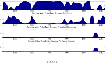
Our main interest is in which of the four forecasts has been best at each point in time. To shed light on this, Figure 2 presents smoothed estimates of the probabilities,
Pr st =kjyT for k = 1; ::;4 and t = 1; ::; T using the switching Gaussian state space model.
In the periods when the consumer survey forecasts receive low probability in Figure 2, it is typically the time series econometrician’s forecasts which are chosen. The one exception to this pattern is the disin‡ationary period of 2008-2009 associated with the …nancial crisis and subsequent recession. This is the one period where the professional forecasts and no change forecasts (receiving roughly equal probability) are being selected by the switching state space model. An examination of the original data (see Figure 1), reveals that both of these forecasts adjusted more rapidly to the disin‡ation which occurred at this time. However, by the middle of 2009 the professionals and the naive forecasts are again being beaten by the consumer survey and the time series econometrician.
1985 1990 1995 2000 2005 2010 0
0.5 1
Smoothed Model Probabilities, Regressor: Consumer Survey
1985 1990 1995 2000 2005 2010 0
0.5 1
Smoothed Model Probabilities, Regressor: Time Series
1985 1990 1995 2000 2005 2010 0
0.5 1
Smoothed Model Probabilities, Regressor: Professional Forecasters
1985 1990 1995 2000 2005 2010 0
0.5 1
[image:10.595.131.569.317.584.2]Smoothed Model Probabilities, Regressor: No Change Forecasts
Figure 2
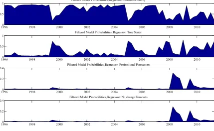
The model probabilities in Figure 2 are smoothed estimates based on the entire sam-ple. Such a …gure is of interest for a retrospective analysis where the researcher looks back on past forecast performance. It is also interesting to present …ltered estimates,
Pr (st=kjyt), so as to show which forecasts a researcher in time t (given information available at timet) would have thought were good ones.3 Figure 3 presents these …ltered probabilities. It can be seen that the main patterns in Figure 3 are broadly similar to
3The …ltered probabilities are calculated by repeatedly running the MCMC algorithm on an expanding
Figure 2. The consumer survey tends to receive the most probability, followed by the forecasts of the time series econometrician. Periods where the consumer survey is not se-lected are usually recessionary or unstable times. The main di¤erence is post-2007 where the …ltered probabilities are very erratic and indicate the no change forecasts would never have been chosen. The professional forecasters have a brief period of higher probability shortly after the …nancial crisis, but it is shorter than in Figure 2.
19960 1998 2000 2002 2004 2006 2008 2010 0.5
1
Filtered Model Probabilities, Regressor: Consumer Survey
19960 1998 2000 2002 2004 2006 2008 2010 0.5
1
Filtered Model Probabilities, Regressor: Time Series
19960 1998 2000 2002 2004 2006 2008 2010 0.2
0.4
Filtered Model Probabilities, Regressor: Professional Forecasters
19960 1998 2000 2002 2004 2006 2008 2010 0.2
0.4
[image:11.595.134.564.264.527.2]Filtered Model Probabilities, Regressor: No change Forecasts
Figure 3: Using Switching State Space Model
3.3.1 Comparison to DMA and DMS using Forgetting Factors
Raftery et al (2010) introduce an algorithm for doing DMA or DMS which involves the use of forgetting factors. There has been a recent surge in popularity in using forgetting factor methods for model averaging with empirical researchers (see, e.g., Dangl and Halling, 2012, Koop and Korobilis, 2012, Koop and Tole, 2013, McCormick, Raftery, Madigan and Burd, 2012, Nicoletti and Passaro, 2012 and Koop and Korobilis, 2013). Raftery et al (2010, page 53) stress that their methods are not a special case of a switching state space model such as the one used in the present paper, but are closely related. The switching state space model approach involves speci…cation of a matrix of Markov transition probabilities,
ij = Pr (st=ijst 1 =j). The forgetting factor approach does not do so. In cases where
the number of models is very large, parsimony considerations mean fully specifying such a matrix is not sensible. The switching state space model involves use of MCMC methods. The forgetting factor approach leads to a …ltering algorithm which does not use MCMC. In large model spaces, the computational burden of MCMC methods mean they need to be avoided. Nevertheless, the goal of our switching state space model and Raftery et al (2010)’s approach is the same: to obtain a method for model selection or model averaging done in a time varying manner.
The references in the preceding paragraph all contain empirical applications with large model spaces where forgetting factor methods are used. But they do not contain com-parisons of the forgetting factor approach with a formal Bayesian model which allows for dynamic model change. With large model spaces this would be computationally infeasi-ble. But with a small model space such as the one used in our empirical application such a comparison can be done. Our aim is to shed light on whether forgetting factor methods lead to similar empirical results as a formal Bayesian approach.
Since forgetting factor methods are established in the literature, we will not provide a description of them here. The reader unfamiliar with DMA using forgetting factors is referred to Raftery et al (2010) or they can read the brief description provided in Appendix B of this paper. Speci…cation details, such as forgetting factor choices, are discussed in this appendix.
It is important to note that the algorithm of Raftery et al (2010) is a …ltering algo-rithm. As described in Appendix B, It provides us with tjt;j which is the probability that model j generated at time t, given information through time t. This a similar concept to
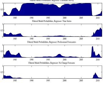
Figure 4 should be compared to Figure 3. In a very broad sense, Figures 3 and 4 tell the same story. Most of the time the consumer surveys are providing the best forecasts for in‡ation. The times when the consumer surveys are not forecasting best tend to be unstable or recessionary times. The forecasts of the time series econometrician also receive appreciable weight, especially at the beginning and end of the sample.
However, there are many details in which Figures 3 and 4 di¤er. Most prominently, the professional forecasters do better in Figure 4 than they did in Figure 3. There are times, most particularly at the beginning and end of the sample, where the forgetting factor approach allocates considerable weight to their forecasts. The second interesting di¤erence is that the switching state space model seems more capable of capturing abrupt switches in model probabilities. For instance, there are several times in Figure 3 when the probability attached to the consumer surveys switched abruptly from near one to near zero or vice versa (e.g. around 1990, 2000 and 2005). These abrupt switches do not appear using the forgetting factor approach. However, the abrupt switch associated with the …nancial crisis does appear in both Figures 3 and 4.
1985 1990 1995 2000 2005 2010 0
0.5 1
Filtered Model Probabilities, Regressor: Consumer Survey
1985 1990 1995 2000 2005 2010 0
0.5 1
Filtered Model Probabilities, Regressor: Time Series
1985 1990 1995 2000 2005 2010 0
0.5 1
Filtered Model Probabilities, Regressor: Professional Forecasters
1985 1990 1995 2000 2005 2010 0
0.5 1
[image:14.595.133.471.131.410.2]Filtered Model Probabilities, Regressor: No Change Forecasts
Figure 4: Using Raftery et al (2010)
3.4
Forecasting Comparison of Di¤erent Implementations of DMA/DMS
In this sub-section we compare the one-step ahead forecasting performance of our di¤erent implementations of DMA and DMS. For the switching Gaussian state space model, we repeatedly run our MCMC algorithm on an expanding window of data to provide forecasts ofytusing information available at timet 1and use this to calculate the one-step ahead predictive density. The output from this procedure can be thought of as a DMA procedure where we are averaging over st=f1; ::;4g. We can also obtain the predictive density for the value of st with highest posterior probability, a strategy analogous to DMS.
window of data for a constant coe¢ cient model. The second of these allows for a large degree of model switching and time variation in parameters. With regards to the error variance, we use both heteroskedastic and homoskedatic estimates (see Appendix B). The former of these are obtained using a rolling window of 10 observations, the latter an expanding window of data.
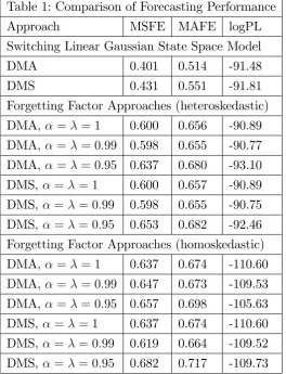
To evaluate our forecasts we use mean squared forecast errors (MSFEs) and mean absolute forecast errors (MAFEs) which evaluate the quality of the point forecasts. MSFEs for any approach are presented relative to the MSFE of the no change forecast. To evaluate the quality of the entire predictive density, we also present sums of log predictive likelihoods (logPL). We evaluate our forecasts over the period 1996Q1 to the end of the sample.
Several patterns emerge from Table 1. The sum of log predictive likelihoods would be the preferred Bayesian method of forecast comparison and it indicates that the forgetting factor approach forecasts slightly better than the switching linear Gaussian state space model, provided we allow for heteroskedasticity and do not choose forgetting factor values which allow for too much variation in the coe¢ cients or too much model switching. That is, the forgetting factor method using the benchmark = = 0:99 choices used by Raftery et al (2010) lead to the best forecast performance (although the = = 1 which leads to conventional BMA in a constant coe¢ cient model on an expanding window of data forecasts only slightly worse). Homoskedastic variants of DMA or DMS forecast quite poorly, emphasizing the importance of allowing for heteroskedasticity.
However, if we look at MSFEs and MAFEs, then a di¤erent pattern emerges where the switching linear Gaussian state space model forecasts appreciably better than forgetting factor approaches. Thus, the former methods are better at producing point forecasts. However, forgetting factor methods are clearly doing well in getting higher order moments and the entire shape of the predictive density correct.
Table 1: Comparison of Forecasting Performance Approach MSFE MAFE logPL Switching Linear Gaussian State Space Model
DMA 0.401 0.514 -91.48
DMS 0.431 0.551 -91.81
Forgetting Factor Approaches (heteroskedastic) DMA, = = 1 0.600 0.656 -90.89 DMA, = = 0:99 0.598 0.655 -90.77 DMA, = = 0:95 0.637 0.680 -93.10 DMS, = = 1 0.600 0.657 -90.89 DMS, = = 0:99 0.598 0.655 -90.75 DMS, = = 0:95 0.653 0.682 -92.46 Forgetting Factor Approaches (homoskedastic) DMA, = = 1 0.637 0.674 -110.60 DMA, = = 0:99 0.647 0.673 -109.53 DMA, = = 0:95 0.657 0.698 -105.63 DMS, = = 1 0.637 0.674 -110.60 DMS, = = 0:99 0.619 0.664 -109.52 DMS, = = 0:95 0.682 0.717 -109.73
In summary, our forecasting results are somewhat mixed. For the researcher interested in point forecasts, the fully Bayesian estimation procedure for switching state space models is to be preferred since it is leading to substantially lower MSFEs and MAFEs. However, for the researcher interested in the entire predictive density, DMA and DMS methods using forgetting factors are forecasting very well indicating that the approximations and compromises inherent in forgetting factor approaches do not carry a large cost with them.
3.5
Forecasting Comparison of Di¤erent Implementations of DMA/DMS
in a Larger Model Space
…ltered estimates of model probabilities, comparable to Figures 2 and 3 indicate that consumer surveys and time series econometrics forecasts still dominate (sometimes in-dividually, sometimes in the model containing the two explanatory variables CS
t and T S
t ).
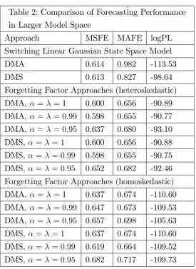
Table 2 presents sums of log predictive likelihoods, MSFEs and MAFEs for the same set of approaches as in Table 1. The message of Table 2 is clear. DMA or DMS done using forgetting factor methods is yielding virtually the same results in Tables 1 and 2. However, the forecasting performance of approaches based on the switching linear Gaussian state space model have deteriorated substantially.
In this empirical application, where we usually …nd models with a single explana-tory variable to forecast best, the parsimonious forgetting factor approach is successfully choosing these models and ignoring the less parsimonious models with several explanatory variables. However, the switching linear Gaussian state space approach is not. Remember that the latter approach involves estimating a 15 15 matrix of transition probabilities. With our relatively short data set, the switching Gaussian state space model is over-parameterized and this is leading to poor forecasts.
Table 2: Comparison of Forecasting Performance in Larger Model Space
Approach MSFE MAFE logPL Switching Linear Gaussian State Space Model
DMA 0.614 0.982 -113.53
DMS 0.613 0.827 -98.64
Forgetting Factor Approaches (heteroskedastic) DMA, = = 1 0.600 0.656 -90.89 DMA, = = 0:99 0.598 0.655 -90.77 DMA, = = 0:95 0.637 0.680 -93.10 DMS, = = 1 0.600 0.656 -90.88 DMS, = = 0:99 0.598 0.655 -90.75 DMS, = = 0:95 0.652 0.682 -92.46 Forgetting Factor Approaches (homoskedastic) DMA, = = 1 0.637 0.674 -110.60 DMA, = = 0:99 0.647 0.673 -109.53 DMA, = = 0:95 0.657 0.698 -105.63 DMS, = = 1 0.637 0.674 -110.60 DMS, = = 0:99 0.619 0.664 -109.52 DMS, = = 0:95 0.682 0.717 -109.73
4
Conclusions
The Bayesian empirical researcher often faces a trade-o¤ between the desire to work with a fully speci…ed Bayesian model and the computational burden that use of MCMC methods imposes. In the DMA literature, when the researcher works with large model spaces, it is common to use forgetting factor methods because the computational burden of doing MCMC is simply too great. In this paper, we have worked with relatively small model spaces (where MCMC methods are computationally feasible) to investigate the possible consequences of using approximate forgetting factor methods. We set up a fully speci…ed Bayesian approach, using a switching linear Gaussian state model, which allows for model switching or model averaging in time-varying parameter models. This can be thought of as an alternative to doing DMA using forgetting factor methods.
approaches indicate that the consumer survey provides the best forecasts of in‡ation most of the time. However, both of them …nd that time series forecasts and surveys of professionals do tend to forecast better at particular periods (e.g. the recent …nancial crisis and subsequent recession). In terms of forecasting, the two approaches exhibit a similar performance if we use sums of log predictive likelihoods as a metric. However, MSFEs and MAFEs show a deterioration in forecasts for forgetting factor approaches.
When we move to a larger model space of 15 models, the forecasting performance of the switching linear Gaussian state space model deteriorates substantially. This contrasts with the forgetting factor approach where forecast performance is una¤ected by the move to a larger model space. Thus, the switching Gaussian state space model can become over-parameterized even with model spaces of this size.
References
Ang, A., Bekaert, G. and Wei, M. (2007). “Do macro variables, asset markets, or surveys forecast in‡ation better?” Journal of Monetary Economics 54, 1163-1212.
Bates, J. and Granger, C. (1969). “Combination of forecasts,” Operational Research Quarterly, 20, 451-468.
Billio, M., Casarin, R., Ravazzolo, F. and van Dijk, H. (2011). “Combining predictive densities using nonlinear …ltering with applications to US economics data,” Tinbergen Institute Discussion Paper, TI 2011, 172/4.
Chan, J. and Jeliazkov, I. (2009). “E¢ cient simulation and integrated likelihood estimation in state space models,” International Journal of Mathematical Modelling and Numerical Optimisation 1, 101-120.
Chan, J., Koop, G., Leon-Gonzalez, R. and Strachan, R. (2012). “Time varying dimension models,” Journal of Business and Economic Statistics, 30, 358-367.
Chipman, H., George. E. and McCulloch, R. (2001). “The practical implementation of Bayesian model selection,” IMS Lecture Notes Monograph Series, 38, 66-134.
Cogley, T. and Sargent, T. (2005). “Drifts and volatilities: Monetary policies and outcomes in the post WWII U.S.,” Review of Economic Dynamics 8, 262-302.
Cogley, T., Morozov, S. and Sargent, T. (2005). “Bayesian fan charts for U.K. in‡a-tion: Forecasting and sources of uncertainty in an evolving monetary system,”Journal of
Economic Dynamics and Control 29, 1893-1925.
D’Agostino, A., Gambetti, L. and Giannone, D. (2011). “Macroeconomic forecasting and structural change,” Journal of Applied Econometrics, DOI: 10.1002/jae.1257.
Dangl, T. and Halling, M. (2012). “Predictive regressions with time varying coe¢ -cients,”Journal of Financial Economics, forthcoming.
Faust, J. and Wright, J. (2012). “Forecasting in‡ation,”chapter in forthcoming Hand-book of Forecasting.
Fruhwirth-Schnatter, S. (2001a). “Fully Bayesian analysis of switching Gaussian state space models,” Annals of the Institute of Statistical Mathematics 53, 31-49.
Fruhwirth-Schnatter, S. (2001b). “Markov chain Monte Carlo estimation of classical and dynamic switching and mixture models,” Journal of the American Statistical Asso-ciation 96, 194-209.
Fruhwirth-Schnatter, S. (2006). Finite Mixture and Markov Switching Models (New York: Springer).
Guidolin, M. and Timmermann, A. (2009). “Forecasts of US short-term interest rates: A ‡exible forecast combination approach,” Journal of Econometrics 150, 297-311.
later,”Jour-nal of Forecasting 8, 167-173.
Green, P. (1995). “Reversible jump MCMC computation and Bayesian model deter-mination,” Biometrika 82, 711-732.
Hoeting, J., Madigan, D., Raftery, A. and Volinsky, C. (1999). “Bayesian model averaging: A tutorial,” Statistical Science 14, 382-417.
Kim, C.J. (1994). “Dynamic linear models with Markov switching,”Journal of Econo-metrics 60, 1-22.
Kim, C.J. and Nelson, C. (1999). State-Space Models with Regime Switching: Classical
and Gibbs-sampling Approaches with Applications. Cambridge, MA: MIT Press.
Koop, G. and Korobilis, D. (2012). “Forecasting in‡ation using dynamic model aver-aging,” International Economic Review, 53, 867-886 .
Koop, G. and Korobilis, D. (2013). “Large Time-varying Parameter VARs,” Journal of Econometrics, 177, 185-198.
Koop, G., Leon-Gonzalez, R., Strachan, R. (2009). “On the evolution of the monetary policy transmission mechanism,” Journal of Economic Dynamics and Control 33, 997-1017.
Koop, G. and Tole, L. (2013). “Forecasting the European carbon market,”Journal of the Royal Statistical Society, Series A 176, 723-741.
Korobilis, D. (2013). “Assessing the transmission of monetary policy shocks using dynamic factor models,” Oxford Bulletin of Economics and Statistics, 75, 157-179.
McCormick, T., Raftery, A., Madigan, D. and Burd, R. (2012). “Dynamic logistic regression and dynamic model averaging for binary classi…cation,”Biometrics, 68, 23-30. Nicoletti, G. and Passaro, R. (2012). “Sometimes it helps: The evolving predictive power of spreads on GDP,” European Central Bank Working Paper, no. 1447.
Primiceri. G. (2005). “Time varying structural vector autoregressions and monetary policy,” Review of Economic Studies, 72, 821-852.
Raftery, A., Karny, M. and Ettler, P. (2010). “Online prediction under model uncer-tainty via dynamic model averaging: Application to a cold rolling mill,” Technometrics, 52, 52-66.
Appendix A: Bayesian Inference in the Switching Linear Gaussian
State Space Model
The switching linear Gaussian state-space model the we adopt is of the form:
p(s1 =k) = K1
jk =p(st =kjst 1 =j) 1 N(0K;2IK)
t = t 1+ t
yt =ZtG[st=k] t+"t;
fort= 1; ::; T andj; k = 1; ::; K. Error assumptions and de…nitions ofst2 f1; ::; Kg; yt; Zt and G[st=k] are given in Section 2. The remaining parameters of the model are =
( 2
1; : : : ; 2K;
2[1]
" ; : : : ; 2["K]; 11; ::; KK)0. We adopt a notational convention for data and states such that subscripts denote a particular time period and superscripts denote all periods up to that time period. For instance,st = (s
1; ::; st)0 denotes all regime indicators up to time t.
We use the Gibbs sampler that sequentially draws fromp TjyT; sT; ,p sTjyT; T;
and p jyT; sT; T . This technical appendix brie‡y describes each of these conditional posterior densities. The time-varying parameters are drawn from p TjyT; sT; using the algorithm of Chan and Jeliakov (2009). Andp sT
jyT; T; is drawn as in Fruhwirth-Schnatter (2001a,b). We refer the reader to page 420 of Fruhwirth-Fruhwirth-Schnatter (2006) for speci…c details of implementation. Note that this algorithm deliversp ytjst; t; which, when averaged over Gibbs draws, provides us with an estimate of the predictive likelihood.
For p jyT; sT; T
we use conditionally conjugate priors which lead to the following conditional posteriors. Given inverted Gamma priors for 2
k (for k = 1; ::; K) with prior hyperparameters c0k and C0k we obtain and inverted Gamma posterior with arguments:
ck(S) = c0k+ T2; Ck(S) = C0k+
PT
t=1( k;t+1 k;t)
2
2 :
We set the prior hyperparameters toc0k = 5 and C0 = [0:08;0:148;0:45;0:53].
For 2["k] we also use inverted Gamma priors leading to inverted Gamma conditional
posteriors. We set prior hyperparametersc[0k"]andC0[k"]toc[0k"]= 5andC0[k"]= [0:168;1:480;7:2;10:0], for k = 1; ::; K. The resulting posterior has arguments
c"[k](S) = c[0k"]+N2kk; C"[k](S) = C0[k"]+ 12PTt:st=k yt ZtG[st=k] t
2
whereNjk counts the number of transitions fromj tok. If j =k it counts the number of periods spent in regimek.
Finally, let be the matrix of Markov transition probabilities jk and let j be thejth row of this matrix. The conditional conjugate prior for each row is Dirichlet:
j D(ej1; : : : ; ejK); j = 1; : : : ; K:
Following Fruhwirth-Schnatter (2001b), we adopt a prior re‡ecting a belief that the prob-ability of staying in a regime is greater than the probprob-ability of transition to a new regime. Thus, we set ejj; j = 1; : : : ; K corresponding to the main diagonal to be 4. Hyperpara-meters o¤ the main diagonal, eji; j 6= i, are set to 0:33. With this choice of prior, the conditional posterior is also Dirichlet with
Appendix B: Dynamic Model Averaging Using Forgetting
Fac-tors
This appendix brie‡y outlines the main features of the DMA algorithm of Raftery et al (2010) as we implement it in this paper.
Suppose we have j = 1; ::; K TVP regression models,
yt = Z
(j)
t
(j)
t +"
(j)
t
(j)
t+1 = (j)
t +
(j)
t ;
"t(k) isN 0; Ht(j) and (tk) isN 0; Q
(j)
t . We replaceH
(j)
t by a simple estimate (the sum of squared errors divided by sample size).
If Q(tj) were known, then an individual model could be estimated in a straightforward manner using the Kalman …lter. Q(tj)appears in the Kalman …ltering prediction equation. In particular, if yt= (y
1; ::; yt)0, then:
(j)
t jyt 1 N tjt 1; Vtjt 1 ;
where
Vtjt 1 =Vt 1jt 1+Q (j)
t :
This is the only place whereQt enters the Kalman …ltering formulae. If the equation for
Vtjt 1 is replaced by:
Vtjt 1 =
1
Vt 1jt 1;
then MCMC methods can be avoided. is a forgetting factor. Forgetting factors have long been used in the state space literature to simplify estimation. There are many ways of justifying the use of forgetting factors as leading to sensible approximations. For instance, their use in this context implies that observations j periods in the past have weight j. An alternative way of interpreting is to note that it implies an e¤ective window size of
1
1 .
for tjt 1;j. A recursive algorithm involving tjt;j and tjt 1;j can be run, beginning with
0j0;j in order to provide the necessary model probabilities. Note that tjt 1;j is a similar concept to the Pr (st=kjyt 1) used in the switching state space model and can be used in the same manner.
Raftery et al (2010) derive a model updating equation of:
tjt;j =
tjt 1;jpj(ytjyt 1)
PJ
l=1 tjt 1;lpl(ytjyt 1)
;
where pj(ytjyt 1) is the predictive likelihood for modelj produced by the Kalman …lter. However, instead of using a Markov transition matrix to model the probability of switching between models, a model prediction equation involving a forgetting factor is used:
tjt 1;j =
t 1jt 1;j
PJ
l=1 t 1jt 1;l
:
This algorithm has a large advantage in that no MCMC is required and a complete speci…cation of a Markov transition matrix is not required. It is computationally e¢ cient, involving only the …ltering algorithms just described. Its properties are described in more detail in Raftery et al (2010).