This is a repository copy of
Regional Interest Rate Pass-Through in Italy
.
White Rose Research Online URL for this paper:
http://eprints.whiterose.ac.uk/95225/
Version: Accepted Version
Article:
Montagnoli, A., Napolitano, O. and Siliverstovs, B. (Accepted: 2015) Regional Interest
Rate Pass-Through in Italy. Regional Studies. ISSN 0034-3404
https://doi.org/10.1080/00343404.2015.1022311
Reuse
Unless indicated otherwise, fulltext items are protected by copyright with all rights reserved. The copyright exception in section 29 of the Copyright, Designs and Patents Act 1988 allows the making of a single copy solely for the purpose of non-commercial research or private study within the limits of fair dealing. The publisher or other rights-holder may allow further reproduction and re-use of this version - refer to the White Rose Research Online record for this item. Where records identify the publisher as the copyright holder, users can verify any specific terms of use on the publisher’s website.
Takedown
If you consider content in White Rose Research Online to be in breach of UK law, please notify us by
Regional interest rate pass-through in Italy
∗
Alberto Montagnoli Oreste Napolitano
Department of Economics, Department of Economic Studies, S. Vinci University of Sheffield, University of Naples ”Parthenope”,
S10 2GW, UK Naples, 80133, Italy a.montagnoli@sheffield.ac.uk napolitano@uniparthenope.it
Boriss Siliverstovs
ETH Zurich
KOF Swiss Economic Institute Leonhardstrasse 21 8092 Zurich, Switzerland
siliverstovs@kof.ethz.ch
February 18, 2015
Abstract
This paper estimates the pass-through and speed of adjustment of Italian regional interest rates to changes in the money market rate for the period 1998Q1-2009Q4. The main findings suggest that the markup for the lending rates that banks charge are generally higher in the South than in the North. Moreover, the empirical results indicate that the pass-through tends to be longer in Southern regions. Furthermore, this paper finds a little support for the hypothesis that regional banks react asymmetrically when adjusting their loan rates when these are above or below equilibrium levels, but detects some evidence supporting an upward rigidity in the regional deposit rates.
Keywords: Interest rates pass-through; monetary policy, error correction model. JEL classification: E43, E50, R11.
1
Introduction
The common practice of implementing monetary policy in the industrialised countries is through
market-oriented instruments designed to influence short-term interest rates. By setting the official rate central
banks influence short-term money market rates which further feed into consumer and business lending
rates set by commercial banks and other financial institutions. Through changes in the retail rates,
the desired effect on aggregate domestic demand and output is achieved. In these circumstances, the
monetary policy can only be successful if changes in the official interest rate are quickly transmitted to
market retail rates and this pass-through is complete.
There are several stylised facts regarding the nature of the interest rate pass-through that are
docu-mented in the relevant literature. The pass-through may not be always full and instantaneous (de Bondt,
2005; Fuertes and Heffernan, 2009), and it may differ across various types of financial institutions and
financial products (Bredin et al., 2002; Heffernan, 1997; Cottarelli and Kourelis, 1994). In addition,
there are likely asymmetries in the speed of adjustment depending on whether interest rates increase or
decrease (Liu et al., 2008; Chong et al., 2006; Hofmann and Mizen, 2004; Scholnick, 1996). Reaction of
retail interest rates has been found to depend also on size of the policy interest rate changes (Fuertes
et al., 2010; De Graeve et al., 2007).
In this work, the attention is drawn to another aspect of the interest rate pass-through, which so
far has been largely ignored by the empirical literature. While it is commonly acknowledged that the
effectiveness of monetary policy may vary across countries (van Leuvensteijn et al., 2008; Sorensen and
Werner, 2006; Sander and Kleimeier, 2006, 2004, 2002; Mojon, 2000; Cottarelli and Kourelis, 1994), the
possibility that the nature of interest pass-through process could be heterogeneous at the intra-national
level received much less attention. One of the possible reasons is the constraints posed by data limitations
at a regional level, see e.g. Dow and Montagnoli (2007); nevertheless one could expect that, especially
in large countries with heterogeneous regional economic structures, the interest rate pass-through may
vary from region to region. In fact, the regional credit market depends on the regional composition of the
financial sectors, hence the supply curve may differ across regions and therefore a change in the official
interest rate can affect the cost and availability of credit more in some regions than others.
regions, represents a good case for studying the interest rate channel of monetary policy at a regional
level. While there is a number of studies investigating the setting of retail interest rates in Italy, the
monetary transmission mechanism at the regional level has not been investigated in a systematic and
rigorous manner so far.
Previous research on the determinants of retail interest rate settings in the banking industry in Italy
can be summarised as follows. Hester and Sdogati (1989), using quarterly data on average loan and
deposit rates for five large regions, studies the Italian banking system before the starting of the European
Single Market. Hester and Sdogati (1989) point out that there were substantial loan rate differentials
between southern and northern Italian regions. During the period 1969—1987 the median loan rates
where persistently higher—on average by 200 basis points— in the Mezzogiorno than in the Northern
Italy. According to Hester and Sdogati (1989), during the period of investigation there were also observed
regional differentials in deposit interest rates with the average deposit rates being lower in the South than
in the North of the country.
Using a sample of 73 banks for the period from 1993Q3 until 2001Q3, Gambacorta (2008) investigates
the micro and macroeconomic factors that influence the settings of individual bank interest rates in Italy;
his findings suggest the presence of short-run heterogeneity in the price-setting behaviour of banks. More
importantly for the present study, Gambacorta (2008, p. 794) notices that there has been a strong and
persistent dispersion of rates among banks; however no systematic attempt has been carried out in order
to identify whether this dispersion is related to the geographical location of the banks. Using aggregate
data Gambacorta and Iannotti (2007) examine the reaction of rates on short-term loan, current accounts,
and the three-month interbank rates to changes in the repo rate during the period 1985-2002. Their main
finding is that the asymmetric reaction of banks to tightening and easing of monetary policy disappeared
in Italy after the introduction of the 1993 Consolidating Law on Banking.
Cottarelli et al. (1995) address the determination of bank lending rates in Italy during the period
1987-1993. Utilizing data from 63 banks they report that the stickiness of Italian lending rates was
higher than in other countries. They identify the degree of concentration of the regional loan markets
as one of the main factors determining the price rigidity across the Italian banking. Based on this
evidence, Cottarelli et al. (1995, p. 22) make an indirect conjecture that bank geographical location may
correlation analysis between lending rates in Southern and Northern Italy with the level of the treasury
bill rate, they tentatively suggest that the South adjusts slower than the rest of the country. However,
no formal econometric investigation has been carried out in order to verify this hypothesis.
this paper contributes to the debate on the regional transmission mechanism of monetary policy in
Italy by providing empirical evidence on the interest rate pass-through at the intra-national level. To this
end, the unique data set is utilised that comprises short- and long-term lending rates as well as deposit
interest rates collected for each of the 20 Italian administrative regions. The quarterly dataset covers
the period from 1998Q1 until 2009Q4. This dataset has not been used so far to investigate the interest
rate pass-through. In particular, this study is the first that formally tests the long term pass-through,
mark-up and the speed of adjustment at the regional level.
The main findings indicate that the markup for the lending rates are generally higher in the South
than in the North, reflecting the well-documented structural imbalances between these two parts of the
country. Furthermore, the empirical results suggest that the pass-through tends to be longer in the
South than in the North. This paper finds a little evidence supporting the hypothesis of asymmetric
adjustment in the lending rates, but detects some evidence supporting an upward rigidity in the regional
deposit rates.
The remainder of the paper is organized as follows: Section 2 discusses regional aspects of monetary
policy and provides some background on the credit market in Italy and its regions. Section 3 presents
the data, Section 4 and 5 show the methodology and describe the results, respectively. The last section
concludes.
2
Regional aspects of monetary policy and its relevance for Italy
The empirical literature on pass-through has so far ignored the possibility of a regional lending channel; as
discussed in Dow and Montagnoli (2007), the regional credit market depends on the regional composition
of the financial sectors, hence supply curves may differ across regions. Therefore, a change in the official
2.1
Regional aspects of monetary policy
The credit channel literature identifies various mechanisms which create the basis for a regional
transmis-sion of monetary policy. First, banks in some regions might have a less liquid balance sheets making them
more sensitive to changes in interest rates. Second, conditions in regional credit markets may also have
different implications for banks operating nationwide because of the region-specific effects of monetary
policy on perceived lenders risks. As Dow and Montagnoli (2007, p. 3) suggest “...this will depend not
only on the state of local industry, but also on asset values for collateral and on the banks knowledge
capacity. Asset values might be hit harder by a rise in interest rates in peripheral regions, encouraging
capital outflow which reinforces this weakening of values. Further, different depths of knowledge with
respect to remoter regions on the part of national and local banks, where the latter are present, can be a
key factor for credit creation there.” Third, a higher incidence of small and medium enterprises (SMEs)
in certain regions makes them more dependent on local credit supply. There is scope then for the banks
to exercise discriminatory monopoly power. Finally, a growing empirical literature finds that regional
financial activities are important for regional economic growth.1 As it has been found that the
availabil-ity of credit and interest rate on loans are not equal among regions, and local financial development is
important in fostering the generation of entrepreneurship and promoting the growth of firms.
It is important to emphasize the role of the interbank market on the allocation of financial resources
among the Italian regions. The correct functioning of the interbank markets is the sine qua non of
modern financial systems. Their purpose is to efficiently allocate liquidity among financial institutions
at the national and regional levels. In developed economies, interbank rates typically can be seen as an
important benchmark for setting interest rates of other financial products. Mistrulli (2005, p.6) asserts
that “the relevance of the interbank market in Italy does not show a clear pattern overtime: the interbank
assets to total assets ratio ranged from 17 to 21 per cent over the 1990-2003 period. This suggests that
financial consolidation might be neutral in terms of interbank market size: liquidity scale economies and
the transformation of among bank financial linkages into within bank ones have almost been compensated
by an increasing relevance of internal capital markets. Thus, on the base of aggregated data, one would
tend to conclude that the structure of the market has remained substantially stable. However, a closer
look at the data reveals that the interbank market underwent major structural changes”. Nevertheless,
1
due to the size and the geographic composition of Italian banks, larger banks (mostly banks in the North)
negotiate on a bilateral basis even at the cross-border level while small banks have a limited opening to
foreign markets.
The literature further indicates that restrictions on the capital mobility,per se, may not be the only
reason to explain the spatial dimension of financial activities (see e.g. Alessandrini et al., 2008). The
relevance of local financial development seems to remain even if there are no regulatory geographical
re-strictions on the movement of financial capital, suggesting the presence of other types of frictions (Dow,
1992). Particularly, as argued by Roberts and Fishkind (1979), the spatially unbalanced allocation of
credit of national banks might be driven by their efficiency and effectiveness to analyse the
creditwor-thiness of local borrowers and by their ability to monitor local borrowers during the existence of loan
contracts. If the quality of the information-generation process were a decreasing function of the
dis-tance between individual banks and borrowers, banks would have a hierarchy lending preference towards
borrowers in close proximity ( ¨Ozyildirim and ¨Onder, 2008). Finally, as suggested in Rodr´ıguez Fuentes
(1998), the willingness of national banks to lend is directly related to the perceived regional risks and the
difficulty to assess such risks.
2.2
The Italian economic and banking system: some stylized facts
It is a well-known fact that Italy is characterized by significant structural imbalances across regions (see
e.g. Bank of Italy, 2009). In particular, these differences are at most pronounced along the North-South
axis of the country. For example, the South includes 37% of Italy’s population, but it produces only
about a quarter of its gross domestic product. A snapshot of the regional characteristics is presented
in Table 1. GDP per capita in the northern part of the country is more than double the value than
in some of the southern regions (for instance Lombardy shows a value of EUR 27,480 against the EUR
13,349 and EUR 13,748 of Campania and Sicily, respectively). In the southern regions the unemployment
rate is significantly higher than in the North. Finally, there is a smaller amount of bank deposits and
the concentration of bank branches is less pronounced in the South.2 These data portrait a picture
of deep regional heterogeneity in the Italian economy. Therefore it is conceivable that these regional
2An additional information on evolution of the number of banks in Italy and the associated regional differences in branch
characteristics play an important role in explaining why monetary policy may be transmitted differently
from region to region.
[TABLE 1 ABOUT HERE]
Another important characteristic of the regional financial system is the strong perseverance of wide
interest rate differentials, reflecting historically determined conditions that each region operates almost
as a closed and independent financial system with a very little opportunity for arbitrage.
One can identify several factors, both on the demand- and supply-side which could explain why
regional arbitrage is inhibited in Italy; from the demand side one can relate them to size of the firms, the
corporate governance and business environment aspects of the Italian economic system. Firstly, thesize
factor relates to the existence of accession limits to credit among firms. Although SMEs comprise the
majority of firms in Italy, the heterogeneous composition of the firms’ size across regions and the close
link between access to credit and size could prevent regional arbitrage.3 The share of SMEs to the total
number of firms is 60% in the North against a 70% of the South, with Calabria and Sicily showing a
value close to 80% (Alessandrini et al., 2010).
The second factor relates to the governance of the firms and the ability to recruit funds for investment.
Family enterprises account for approximately 83% of the number of medium and small capital enterprises
(Corbetta et al., 2002); they are characterized by a close relationship with the local financial system,
mainly banks, and typically they are prepared to accept higher financing costs in order to preserve their
financial independence and flexibility.
Finally, the last factor is related to the geographic location of the firms; this is what one can refer
to as the business environment factor and ethical behaviour. To access bank financing firms require to
disclose credible information through formal documentation. This requirement might be impossible to
produce if entrepreneurs employ irregular workers or, more generally, they operate, at least partially, in
the underground economy. The distribution of the shadow economy in Italy is heterogeneous both at a
sectoral and at a regional level.4 For example, as shown in Table 1, regions in the South are more affected
3
The composition of the firms by legal status at regional level are individual firms followed by partnership firms and corporations.
4Some economic sectors have a higher propensity to employ irregular workers; for instance, the agriculture and the
by informal economy with rates of irregular workers above the 20% for the period 2001-2008.
The economic environment and the characteristics of the demand-side alone cannot explain the
seg-mentation of the financial system. Alongside the intrinsic problem of adverse selection characterizing
the relationship between banks and entrepreneurs, the structure and the nature of the financial system
across Italy play also a vital part. Firstly, the southern regions banking system share a similar
struc-ture, characterized by high levels of costs (on average) and high level of socio-economic risks. In fact, a
comparatively higher level of concentration in the South compared to the Centre-North has reduced
com-petition allowing the banking system to take advantage of higher interest premia. D’Onofrio and Pepe
(1990) and Jossa (1996) show that, starting from the early fourties and at least until the early nineties,
the southern banking system has been characterized by a relatively low degree of competition. In the
South the financial system has been dominated by only two market players, Banco di Napoli and Banco
di Sicilia. The residual market shares, consisting of small local banks, has been characterized by highly
fragmented supply, with a low level of efficiency, and thus unable to lead to any downward pressure on
the lending rates. Moreover, low level of competition resulted in stronger downward pressure on interest
rates on deposits.
A second supply-side factor deals with the level of the costs incurred by banks.5 Higher operating
costs are likely to lead to comparatively high lending rates. In this sense, the higher direct costs and the
lower productivity of the southern banks may help to explain the existence of an earning margin higher
than the national average. The mergers and acquisitions process which took place during the period
1996-2010 seems to have had a deeper impact in the South with a marked reduction in the number of
local banks (Bank of Italy, 2009). In fact, at the end of 2009, 788 banks were operating in Italy, 53 fewer
than in 2000. This new credit market has not yet determined significant changes in the characteristics of
the southern banking system and the bank-firm relationships. In the South the earning margins remain
higher than the national value and the degree of market concentration has not changed substantially.
Furthermore, the southern regions remain (in spite of a similar propensity to save as in the rest of the
country) markets where banks collect deposits and use them to provide liquidity in other regions that
are less-risky or more profitable.
The lack of arbitrage driven both by the established credit demand- and supply side structures make
regions to function like a close system, where the monetary transmission mechanism is likely to be highly
segmented. Results of the formal investigation of this hypothesis is presented in the following sections.
3
Data
The dataset comprises of short- and long-term business loans rates (excluding mortgages) and deposit
rates for each Italian region collected through a survey by the Bank of Italy on a quarterly basis over the
period 1998Q1—2009Q4.6 The money market rate represents the three-month interbank rate in Italy
(line 60B, IMF International Financial Statistics), calculated as an arithmetic average of daily rates.
Daily rates are computed as weighted averages of rates based on daily transaction volumes. The data are
compiled by the Bank of Italy.
Short- and long-term lending rates refer to revocable loans based on distribution by customer location
(region) and total credit granted. The interest rates is the gross annual percentage (rate paid on loans
by the ordinary customers)7reported by the Bank of Italy in the last month of the quarter. Information
on lending rates were determined separately for each customer and the amount of loans are equal to or
exceeding 75,000 Euros. The short-term interest rates refer to loans withdrawal in each single quarter
with a maturity less than one year, while the long term loans refer to a maturity greater than a year.
Deposits interest rates are specified as current account deposits based on distribution by customer location
(region) and segment of economic activity (total resident non-bank sectors). They are average rates of
current accounts’ deposits of household and non-financial institutions, recorded at the end of each quarter
(see Bank of Italy, 2006).
[TABLE 2 ABOUT HERE]
The descriptive statistics of the interest rates is presented in Table 2. As it could be seen, on average
the southern regions exhibit higher loan rates than the northern regions. Calabria, for instance, has the
highest value both for short- and long-term rates while Piedmont and Lombardy have the lower values.
Looking at the deposits side, Lazio shows the highest value, while Calabria the lowest. At the same time
6All data are stored in the Bank of Italy’s historical statistical database (BIP). 7
deposit rates paid to bank customers tend to be lower on average in the southern regions compared to
those in the north, which is consistent with the results reported in Hester and Sdogati (1989) for the
earlier period.
4
Methodology
As the starting point, the dynamic relationship between the money market ratextand the administered
bank rateyi,t is formulated in terms of an unrestricted AutoRegressive Distributed Lag (ARDL) model:
yi,t =ci+bi,0xt+bi,1xt−1+aiyi,t−1+εi,t. (1)
As shown in Hendry et al. (1984, Section 2.6) and Wickens and Breusch (1988, Sections I), this ARDL(1,1)
model can be transformed in the following error correction model (ECM):
∆yi,t=−(1−ai)
(
yi,t−1−
1 (1−ai)
ci−(bi,0+bi,1)
(1−ai)
xt−1
)
+bi,0∆xt+εi,t, (2)
allowing to distinguish between long- and short-term effects of monetary policy. The expression in
parentheses represents the long-run or equilibrium relationship between the modelled variables:
yi,t =αi+βixt+ui,t, (3)
which is obtained by settingαi=ci/(1−ai) andβi= (bi,0+bi,1)/(1−ai). The parameterβiis the total or
long-run multiplier. It measures the degree of interest rate pass-through in the long run. Correspondingly,
ifβi is equal to one then the long-run adjustment is complete. In the presence of a not fully competitive
banking system the pass-through is not complete and βi takes values less than one. The parameter
αi measures the constant markup reflecting the difference between the money market interest rate and
the administered interest rates that banks offer to their clients. The magnitude of markup depends on
economic and non-economic factors; the higher is the perceived probability of default the higher would
By settingγi=−(1−ai) andθi=bi,0it is possible to write the ECM in the following compact form:
∆yi,t=γi(yi,t−1−αi−βixt−1) +θi∆xt+εi,t, (4)
where the parameter γi is the short-run parameter that measures how fast these deviations from the
long-run relationship observed in the previous period are corrected in periodt. For such error correction
to take place the coefficient γi should be negative, which requires that ai < 1 in Equation (1). The
parameter θi is the short-run pass-through rate, which measures how much of a change in the money
market rate gets reflected in the administered rates in the same period. As shown in Hendry (1995), one
can calculate the mean adjustment lag (MAL) of a complete pass-through for regionias follows:
MALi= (1−θi)/γi. (5)
Since the error-correction model in Equation (4) is written in a multiplicative non-linear form, which
makes direct estimation of its parameters and the associated standard errors by means of OLS impossible,
one can open the brackets in Equation (4) and write the equation as the following unrestricted
error-correction model:
∆yi,t=γiyi,t−1+α∗i +βi∗xt−1+θi∆xt+ϵi,t, (6)
whereα∗
i =−γiαi and βi∗=−γiβi. The coefficients of Equation (6) can be estimated by ordinary least
squares (OLS) and the values of the long-run parameters given in Equation (4) can be recovered from
αi=−α∗i/γiandβi=−β∗i/γi. However, due to the fact that the long-run parametersαiandβidepend
in a non-linear way on the OLS estimates, the computation of associated standard errors requires an
additional effort. In order to compute these a transformation of Equation (6) is applied as suggested in
Bewley (1979).
In order to account for the fact that Italian regional banks may react asymmetrically when adjusting
their administered rates when they are above or below equilibrium levels (e.g., see Cottarelli et al., 1995;
Chong et al., 2006), a dummy (κ) is introduced into the model that takes the value of one whenui,t>0
reads:
∆yi,t=θi∆xt+γi+κui,t−1+γi−(1−κ)ui,t−1+ϵi,t, (7)
whereγi+andγ−
i capture the error correction adjustment speed when the rates are above and below their
equilibrium values, respectively. A Wald test is then employed to test the null hypothesis of symmetric
adjustmentγi+=γ−
i . Similar to Equation (5) one can also define the asymmetric mean adjustment lags
of a complete pass-through as:
M AL+i = (1−θi)/γi+, (8)
M AL−
i = (1−θi)/γi−. (9)
The parameters of the asymmetric adjustment model in Equation (7) are estimated in two steps.
In the first step the estimate of the error-correction term ˆui,t is obtained using the long-run parameter
estimates ˆαi and ˆβi. In the second step the values of ˆui,t−1are inserted in Equation (7). Its parameters
likewise were estimated using the OLS method.
Observe that the empirical model specification is similar to the one used by Chong et al. (2006).
The crucial difference between the present analysis and Chong et al. (2006) is that here interest rates
are treated as stationary but highly persistent processes, whereas in the latter paper interest rates are
assumed to be integrated of order one, i.e. I(1) variables. The choice of treating interest rates as I(0)
rather than I(1) variables is based on the following considerations. First, the non-stationary I(1) variables
are characterised by the absence of a well-defined mean and ever increasing variance—a pattern usually
not observed for interest rates under normal economic conditions. Secondly, the results of formal testing
for unit roots in the interest rate data in question, as discussed in the next section, support the choice
of treating them as stationary variables. Third, the use of stationary data and the consequence that
the cointegration framework is dispensed in the analysis does not rule out the use of error correction
model in order to distinguish between short- and long-run effects of monetary policy (Hendry et al.
(1984, Section 2.6) and Wickens and Breusch (1988, Section I)). Additionally, as shown in Pesaran and
Shin (1999, p. 405) the ARDL modelling approach is a reliable method for estimation of economic
high persistence. Finally, since in this paper stationary variables the standard asymptotic theory can be
used for parameter estimation and statistical inference.
5
Results
First this paper addresses the order of integration of the modelled variables by deploying the CADF panel
unit root test of Pesaran (2007) that accounts for cross-sectional dependence among regional interest rates.
The results of the test suggest that one can reject the null hypothesis that the regional lending and deposit
rates are I(1) at the usual significance levels. The order of integration of the money market interest rate
is addressed by means of the univariate unit root test of Kwiatkowski et al. (1992). According to the test
outcome, one cannot reject the maintained null hypothesis that money market interest rate is I(0).8
The estimates of the linear error-correction model are presented in left panels of Tables 3—5 for
short-term and long-term lending rates as well as deposit interest rates, respectively. The corresponding
results for the asymmetric ECM are reported in right panels of the tables.9
[TABLES 3—5 ABOUT HERE]
Before going into a detailed discussion of the estimation results it is worthwhile emphasising that
despite a rather parsimonious structure of Equation (4) it has a rather high explanatory power, judging
from the reported values of the adjustedR2 in column (7). Moreover, the coefficients of interest in most
cases are found to be significantly different from zero. An exception is the estimated markup for deposit
rates that are often found close to zero and insignificant.
Next the discussion of the estimation results for the symmetric adjustment model is in place here.
The estimated markups for short- and long-term loans are positive and statistically significant from zero
for all regions. The value of the markup on long-term loans is smaller than the estimates on short-term
loans, reflecting the fact that the latter apply to borrowers with liquidity shortage and the short-term
loans are usually not collateralized. In both sets of results, Calabria shows the highest markups (2.74
8
To save space results are not reported here, but they are available upon request.
9The model assumptions were verified using a battery of regression diagnostic tests, such as the LM test of no residual
and 6.67, respectively); while the smallest value for short-term loans is estimated to be in Trentino-Alto
Adige (2.37) and in Lombardy for the long-term loans (1.54). These results bring support the role played
by the three main factors (conventional, history of the firms and environmental) described in section 2.2
as the reasons why arbitrage is prevented among the regions. The estimated markups for deposits are
negative, although these were found not always significantly different from zero. This suggests that the
banking system tends to offer its depositors a rate or return which is lower than the money market rate.
The estimates of the long-run pass-through coefficientβfor lending rates present a quite heterogeneous
pattern. There are a number of regions for which estimates of β are quite close to unity and therefore
one cannot reject the null hypothesis thatβ = 1. The complete pass-through takes place in Piedmont,
Trentino-Alto Adige, Aosta Valley, Basilicata, Sardinia and Sicily for short-term lending rates and in
Aosta Valley, Campania, Sardinia and Sicily for long-term lending rates. For the rest of the regions one
can reject the null hypothesis, indicating an incomplete pass-through. For the deposit rates, there is a
clear-cut picture. The estimates ofβ are found to be generally lower than those for lending rates. As
a result, for all twenty regions one can reject the null hypothesis of a complete pass-through in deposit
rates. Understanding why this is the case is beyond the scope of this work, but one can conjecture that
two possible explanations are the absence of commutativity in the banking sector and the unwillingness
of depositors to look for the best deal for their savings. This could be the result of both a lower degree
of competition resulting from merges and acquisition process during the last two decades and the
con-sequence of the securitisation process10 that generated a replacement of the traditional bank loans with
forms of financing represented by marketable securities.
The estimates of the adjustment coefficient to the error-correction term, γ, are negative in all cases
suggesting that the correction to the past-period disequilibrium indeed takes place across all regions.11
10The importance of deposits has diminished both for the saver and for the banks. This can be attributed to the process
of securitisation, which took place in the last decades. For savers, bank deposits become only an instrument to keep their cash for day-to-day activities rather than to seek for a yield. Moreover, securitisation, led banks to replace deposits with other financial securities. This resulted in a lower competition among banks for deposits.
11
This adjustment is faster for long rate with an average of −0.64 computed across all regions against
−0.38 and −0.28 for short rates and deposit rates, respectively. In Sicily it takes longer to adjust for
both long-term (−0.15) and short-term rates (−0.25), while the fastest adjustment takes place in Toscana
(−0.48) for short rates and in Lazio for long rates (−0.99). For deposits, the region with the highest
value of adjustment estimate is the Friuli-Venezia Giulia (−0.69) and Abruzzo shows the smallest estimate
(−0.16).
The estimates of the short-term pass-through, given by the values ofθ, are all positive and statistically
significant at the usual levels. The term pass-through is of a similar (average) magnitude for
short-and long-term interest rates, but generally it is higher for lending rates than for deposit rates. Combined
with a higher speed of adjustment to deviations from the long-run relationship for long rates, it is
reasonable to conclude that the transmission of changes in money market rate is fastest for long interest
rates, reflected in the smallest values of the mean adjustment lag.
Next this paper presents the estimation results obtained by relaxing the restriction of a symmetric
adjustment to deviations from the long-run relationship between the administered rates and the money
market rate. In most cases one cannot reject the null hypothesis of a symmetric adjustment. For
short-and long-rates one can reject the corresponding null hypothesis for Trentino Alto Adige short-and Marche,
respectively. It is interesting that most of the evidence on asymmetric adjustment comes from deposit
rate regressions. In this case one can reject the symmetry hypothesis for four regions: Veneto, Emilia
Romagna, Lazio, Puglia. Observe that for all regions for which one can reject the null hypothesis of the
symmetric adjustment, the adjustment speed is slower when rates are below their equilibrium value.
Tables 3—5 report the estimation results for every of 20 Italian regions. The interest of the paper,
however, lies in exploring whether noticeable differences across the regional bank branches operating
in three macro areas (North, Center, and South of Italy) exist. In order to summarise the
heteroge-neous estimation results one can aggregate them by taking simple arithmetic averages of the individual
coefficients’ estimates for each geographical area.
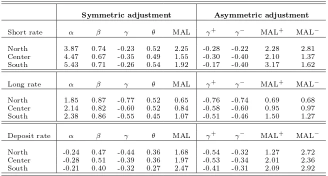
The averages of coefficient estimates the three macroareas (North, Center and South) are reported
in Table 6. The most interesting evidence supporting the idea of importance of regional differences for
monetary policy comes from the markup estimates for short- and long-term lending rates. For these rates
operating in the south demand an extra rent from its customers in order to compensate for a greater risk
of default on loans.
[TABLE 6 ABOUT HERE]
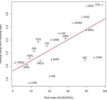
In order to shed more light on this topic, one can relate the estimated markups for lending rates to the
risk index, which was released by the Italian Institute of Political Studies, Economic and Social Affairs
(EURISPES) for 2008. The risk index is a composite indicator summarising a socio-economic condition
for each region in Italy. It is based on the following four categories of the variables such as 1) economic
variables: GDP and unemployment; 2) banking system position: bad debts, average interest rate, number
of bank branches, number of co-operative and “popular” banks, number of home and corporate clients,
local councils served by banks; 3) development of local entrepreneurship: number of sole proprietorships,
new firms, closed down firms; 4) criminality level: extortion and conspiracy to defraud.
The regression results are reported in Equations (10) and (11). Both regressions reveal a rather high
explanatory power of the risk index for estimated markups. The associated values of the adjusted R2
are 0.64 and 0.41 for short- and long-term lending rates, respectively. The corresponding crossplots are
presented in Figures 1 and 2 again revealing a high, positive correlation between the variables of interest.
Markup (short-rate) = 2.963
(0.306)
+ 0.033
(0.005)
Risk index, R2= 0.64.
(10)
Markup (long-rate) = 1.723
(0.118)
+ 0.008
(0.002)
Risk index, R2= 0.41.
(11)
[FIGURES 1 AND 2 ABOUT HERE]
The estimates of the mean adjustment lag (measured in quarters) provide further evidence of the
existence of regional differences in the monetary transmission mechanism in Italy. One finds that both
for long-term lending rates and deposit rates the estimated MAL is on average higher in the south than
in the North. The central regions are again placed in between. For example, in case of long-term lending
rates it takes about two months (0.65) in order fully to accommodate changes in the money market rate
lags for deposit rate is about five months (1.68) and slightly longer than seven months (2.47) in the north
and south, respectively.
For short-term lending rate the finding is that in the South the MAL is on average higher than in
the central regions. At the same time the average of mean adjustment lags estimated for the northern
regions exceeds those observed for the southern and central regions. However, a closer inspection suggests
that for short rate there exists a wide difference between estimates of MAL for the regions in the
north-east (Friuli-Venezia Giulia, Trentino-Alto Adige, Veneto) and the north-west (Aosta Valley, Piedmont,
Liguria, Lombardy). The average value of MAL for the former group of regions is about one and a half
quarters (1.52), that is similar in magnitude to that observed for central regions, against about eight
months (2.62) for the latter group of regions.
Finally, the aggregated results reported in Table 6 also suggest that there is a little systematic evidence
of an asymmetric adjustment to deviations from the long-run relationship among the lending rates and
the money market rate. These findings tend to favour the view that the asymmetric adjustment comes
from estimates obtained for deposit rates. One observes that for all macroareas the averages of individual
estimates are higher forγ+ than forγ−. This finding indicates that the banks adjust their deposit rates
faster when they are above their equilibrium levels rather than when they are below, thus exploiting the
asymmetry in their bank-client relationship. An interesting extension of the current paper would be a
more detailed inquiry in this practice looking for determinants of deposit interest-rate setting behaviour
by individual banks, but this requires a more detailed data set containing characteristics of individual
banks.
6
Conclusions
This paper highlights the importance of regional differences that need to be taken into account when
assessing the effects of monetary policy in large, geographically diverse countries. Due to the fact that
different administrative regions within a country might have different socio-economic conditions or
seg-mented regional credit markets, the credit supply-and demand curves may differ across regions. Therefore
a change in the official interest rate may have heterogeneous effects on the cost and availability of credit.
rather than international level. Using Italy as an example, this paper demonstrates that there exist
substantial differences in how regional banks in the North and South set their administered interest rates
in response to changes in money market rate. The finding that the markup for the bank lending rates
are generally higher in the South than in the North, reflecting the well-documented structural imbalances
between these two parts of the country. Furthermore, the estimation results suggest that the pass-through
tends to be longer in the South than in the North. This paper documents a little empirical support for
the hypothesis of asymmetric rigidity in the loan rates, but detects some evidence supporting an upward
References
Alessandrini, P., G. Calcagnini, and A. Zazzaro (2008). Asset restructuring strategies in bank acquisitions: Does distance between dealing partners matter? Journal of Banking & Finance 32(5), 699–713.
Alessandrini, P., A. F. Presbitero, and A. Zazzaro (2009). Global banking and local markets: A national perspective. Cambridge Journal of Regions, Economy and Society 2(2), 173–192.
Alessandrini, P., A. F. Presbitero, and A. Zazzaro (2010). Bank size or distance: What hampers innovation adoption by SMEs? Journal of Economic Geography 10(6), 845–881.
Bank of Italy (2003). Indagine sul credito bancario. Bank of Italy 2003.
Bank of Italy (2006). Supplementi al bollettino statistico. Anno XVI Numero 11–2, Febbraio 2006.
Bank of Italy (2009). Economic developments in the Italian regions in 2008. Bank of Italy 2009, No. 61.
Bewley, R. A. (1979). The direct estimation of the equilibrium response in a linear model. Economic
Letters 3, 357–361.
Bredin, D., T. Fitzpatrick, and G. O’Reilly (2002). Retail interest rate pass-through - the Irish experience.
The Economic and Social Review 33(2), 223–246.
Chong, B. S., M.-H. Liu, and K. Shrestha (2006). Monetary transmission via the administered interest rates channel. Journal of Banking & Finance 30(5), 1467–1484.
Corbetta, G., L. Gnan, and D. Montemerlo (2002). Governance systems and company performance in italian smes. Working paper isea, Bocconi University.
Cottarelli, C., G. Ferri, and A. Generale (1995). Bank lending rates and financial structure in Italy: A case study. IMF Working Papers 95/38, International Monetary Fund.
Cottarelli, C. and A. Kourelis (1994). Financial structure, bank lending rates, and the transmission mechanism of monetary policy. IMF Working Papers 94/39, International Monetary Fund.
de Bondt, G. (2005). Retail bank interest rate pass-through: New evidence at the euro area level.German
Economic Review 6(1), 37–78.
De Graeve, F., O. De Jonghe, and R. V. Vennet (2007). Competition, transmission and bank pricing policies: Evidence from Belgian loan and deposit markets. Journal of Banking & Finance 31(1), 259–278.
D’Onofrio, P. and R. Pepe (1990). Le strutture creditizie del mezzogiorno. In G. Galli (Ed.),Il sistema
finanziario del Mezzogiorno. Banca d’Italia, Roma.
Doornik, J. A. and H. Hansen (2008). An omnibus test for univariate and multivariate normality. Oxford
Bulletin of Economics and Statistics 70, 927–939.
Dow, S. C. (1992). The regional financial sector: A Scottish case study. Regional Studies 26, 619631.
Dow, S. C. and A. Montagnoli (2007). The regional transmission of UK monetary policy. Regional
Studies 41(6), 797–808.
Ellis, C. N. (1999). The mezzogiorno at the millenium: The outlook for southern Italy in the year 2000. In P. Janni (Ed.),The European Monetary Union: The 1998. The 1998 Edmund D. Pellegrino Lectures
on Contemporary Italian Politics. Council for Research in Values.
Engle, R. F. (1982). Autoregressive conditional heteroscedasticity with estimates of the variance of united kingdom inflation. Econometrica 50, 987–1007.
Fuertes, A.-M., S. Heffernan, and E. Kalotychou (2010). How do UK banks react to changing central bank rates? Journal of Financial Services Research 37(2), 99–130.
Gambacorta, L. (2008). How do banks set interest rates? European Economic Review 52(5), 792–819.
Gambacorta, L. and S. Iannotti (2007). Are there asymmetries in the response of bank interest rates to monetary shocks? Applied Economics 39(19), 2503–2517.
Gobbi, G. and R. Zizza (2007). Does the underground economy hold back financial deepening? Evidence from the Italian credit market. Temi di discussione (Economic working papers) 646, Bank of Italy, Economic Research and International Relations Area.
Godfrey, L. G. (1978). Testing for higher order serial correlation in regression equations when the regressors include lagged dependent variables. Econometrica 46, 1303–1313.
Heffernan, S. A. (1997). Modelling British interest rate adjustment: An error correction approach.
Economica 64(254), 211–231.
Hendry, D. F. (1995).Dynamic Econometrics. Advanced Texts in Econometrics. Oxford University Press.
Hendry, D. F., A. R. Pagan, and J. Sargan (1984). Dynamic specification. In Z. Griliches and M. D. Intriligator (Eds.), Handbook of Econometrics, Volume 2 of Handbook of Econometrics, Chapter 18, pp. 1023–1100. Elsevier.
Hester, D. and F. Sdogati (1989). European financial integration: Some lessons from Italy. Banca
Nazionale del Lavoro 170, 313–344.
Hofmann, B. and P. Mizen (2004). Interest rate pass-through and monetary transmission: Evidence from individual financial institutions’ retail rates. Economica 71, 99–123.
Jossa, B. (1996). Ridurre i tassi d’interesse al sud. In L. Costabile (Ed.),Istituzioni e sviluppo economico
del Mezzogiorno. il Mulino, Bologna.
Kwiatkowski, D., P. C. B. Phillips, P. Schmidt, and Y. Shin (1992). Testing the null hypothesis of stationarity against the alternative of a unit root: How sure are we that economic time series have a unit root? Journal of Econometrics 54(1-3), 159–178.
Liu, M.-H., D. Margaritis, and A. Tourani-Rad (2008). Monetary policy transparency and pass-through of retail interest rates. Journal of Banking & Finance 32(4), 501–511.
Marullo Reedz, P. (1990). La redditivit delle aziende di credito. In G. Galli (Ed.),Il sistema finanziario
del Mezzogiorno. Banca d’Italia, Roma.
Mistrulli, P. E. (2005). Interbanks lending patterns and financial contagion. Unpublished manuscript, Banca d’Italia, Research Department.
Mojon, B. (2000). Financial structure and the interest rate channel of ECB monetary policy. Working Paper Series 40, European Central Bank.
¨
Ozyildirim, S. and Z. ¨Onder (2008). Banking activities and local output growth: Does distance from centre matter? Regional Studies 42(2), 229–244.
Pesaran, M. H. (2007). A simple panel unit root test in the presence of cross-section dependence. Journal
of Applied Econometrics 22(2), 265–312.
Pesaran, M. H. and Y. Shin (1999). An autoregressive distributed lag modelling approach to cointegration analysis. In S. Strøm (Ed.), Econometrics and Economic Theory in the 20th Century: The Ragnar
Frisch Centennial Symposium, Chapter 11, pp. 371–413. Cambridge University Press: Cambridge.
Pesaran, M. H., Y. Shin, and R. J. Smith (2001). Bounds testing approaches to the analysis of level relationships. Journal of Applied Econometrics 16(3), 289–326.
Ramsey, J. B. (1969). Tests for specification errors in classical linear leat-squares regression analysis.
Journal of the Royal Statisitical Society, Series B 31, 350–371.
Rodr´ıguez Fuentes, C. (2005). Regional Monetary Policy. Routledge, London.
Rodr´ıguez Fuentes, C. J. (1998). Credit availability and regional development. Papers in Regional
Science 77(1), 63–75.
Sander, H. and S. Kleimeier (2002). Asymmetric adjustment of commercial bank interest rates in the euro area: An empirical investigation into interest rate pass-through. Kredit und Kapital 35(2), 161–192.
Sander, H. and S. Kleimeier (2004). Interest rate pass-through in an enlarged Europe: The role of banking market structure for monetary policy transmission in transition countries. Research Memoranda 045, Maastricht: METEOR, Maastricht Research School of Economics of Technology and Organization.
Sander, H. and S. Kleimeier (2006). Interest rate pass-through in the common monetary area of the SACU countries. South African Journal of Economics 74(2), 215–229.
Scholnick, B. (1996). Asymmetric adjustment of commercial bank interest rates: Evidence from Malaysia and Singapore. Journal of International Money and Finance 15(3), 485–496.
Sorensen, C. K. and T. Werner (2006). Bank interest rate pass-through in the euro area: A cross country comparison. Working Paper Series 580, European Central Bank.
van Leuvensteijn, M., C. K. Sorensen, J. Bikker, and A. van Rixtel (2008). Impact of bank competition on the interest rate pass-through in the euro area. DNB Working Papers 171, Netherlands Central Bank, Research Department.
White, H. (1980). A heteroscedastic-consistent covariance matrix estimator and a direct test for het-eroscedasticity. Econometrica 48, 817–838.
Table 1: Regional economic and financial variables
GDP per capita Unemployment rate Irregular workersa Bank deposits Criminalitya Population
(in EUR) (in %) (share, in %) (in Mln. EUR per 1000 inhabitant) per bank branch
average over average over average over average over average over average over
1999-2009 1999-2009 2001-2008 1999-2009 2004-2007 1999-2007
Piedmont (PIE) 23335.94 5.81 9.7 10358 229.36 1749
Aosta Valley (VALD) 27248.28 6.32 10.5 11543 173.82 1190
Lombardy (LOM) 27479.64 3.81 8.1 15120 198.69 1624
Liguria (LIG) 21478.33 7.07 12.3 9748 198.44 1779
Veneto (VEN) 24874.20 4.28 8.6 9860 151.82 1487
Friuli-Venezia Giulia (FRI) 23439.38 4.42 10.5 11381 131.32 1363
Trentino-Alto Adige (TREN) 26581.43 3.11 8.7 12809 122.25 1070
Emilia-Romagna (EMIL) 26710.63 3.30 8.1 11675 210.01 1348
Tuscany (TOS) 23048.63 4.99 9.1 10330 186.31 1654
Umbria (UMB) 20040.38 6.18 12.5 8284 144.06 1565
Marches (MAR) 21268.79 4.84 10.2 9320 145.26 1492
Lazio (LAZ) 24539.08 8.83 12.0 14033 183.26 2270
Abruzzo (ABR) 17916.38 8.55 12.4 7486 175.66 2177
Molise (MOL) 15842.21 10.00 18.7 5360 133.62 2402
Campania (CAM) 13349.7 16.05 20.0 6038 392.46 3845
Puglia (PUG) 13999.72 14.27 17.4 5951 181.96 3122
Basilicata (BAS) 14942.66 12.74 19.5 5472 127.18 2287
Calabria (CAL) 13296.55 15.94 26.6 4502 166.16 4028
Sicily (SIC) 13748.13 18.51 20.7 5603 202.01 2969
Sardinia (SARD) 16108.08 13.25 18.7 6779 157.38 2491
North 24919.60 4.97 8.8 17355 187.96 1466
Centre 22253.98 6.12 10.8 8017 176.11 1751
South 14469.58 14.39 19.6 5373 226.59 3021
Notes: All the data were collected from ISTAT regional accounts, http://www.istat.it/conti/territoriali/.
aShare of total number of workers.
bCriminality is number of murders for a million of inhabitants committed by criminal organizations.
Table 2: Descriptive statistics, 1998Q1—2009Q4
North Center South
Short rate MMITa FRIb LIG LOM PIE TREN VALD VEN ABR EMIL LAZ MOL MAR TOS UMB BAS CAL CAM PUG SARD SIC
µ 3.32 6.62 7.08 5.62 6.32 5.81 7.31 6.41 7.32 5.89 6.62 8.26 6.14 6.38 7.25 7.78 8.78 7.82 7.80 7.56 8.03
σ 1.49 0.74 0.46 0.70 0.65 1.35 0.87 0.64 0.82 0.73 0.88 0.78 0.79 0.67 0.93 1.26 1.22 0.57 0.72 1.48 1.03
min 0.74 4.73 5.73 4.37 4.95 3.61 5.57 4.54 5.62 4.42 5.13 6.22 4.90 4.84 5.15 5.63 6.57 6.18 5.58 4.94 5.51
max 5.94 8.69 8.98 8.10 8.51 8.84 9.60 8.74 10.40 8.24 9.60 11.34 8.91 8.84 10.14 11.57 12.25 10.43 10.45 10.78 11.20
Long rate MMIT FRI LIG LOM PIE TREN VALD VEN ABR EMIL LAZ MOL MAR TOS UMB BAS CAL CAM PUG SARD SIC
µ 3.32 4.82 4.91 4.54 4.58 4.87 5.04 4.84 5.22 4.61 4.81 5.24 4.72 4.80 5.11 5.38 5.52 5.25 5.24 5.34 5.28
σ 1.49 1.06 0.99 1.05 1.14 1.09 1.21 1.07 1.34 1.05 1.01 1.32 0.89 0.92 1.15 1.02 1.39 1.56 0.92 1.07 0.98
min 0.74 3.12 3.14 2.14 2.59 3.00 3.21 2.91 3.34 2.89 3.09 3.60 2.97 2.99 3.27 3.56 3.47 3.24 3.23 3.27 3.44
max 5.94 7.32 7.03 6.37 7.10 7.18 7.10 7.31 8.71 6.99 7.49 8.72 6.32 7.00 7.70 7.94 8.88 8.74 7.82 7.59 6.89
Deposit rate MMIT FRI LIG LOM PIE TREN VALD VEN ABR EMIL LAZ MOL MAR TOS UMB BAS CAL CAM PUG SARD SIC
µ 3.32 1.54 1.10 1.42 1.18 1.57 1.32 1.31 1.35 1.35 1.78 1.32 1.40 1.43 1.45 1.18 1.00 1.04 1.16 1.40 1.29
σ 1.49 0.35 0.19 0.29 0.21 0.41 0.26 0.26 0.34 0.25 0.47 0.31 0.28 0.32 0.33 0.23 0.21 0.23 0.23 0.29 0.21
min 0.74 0.37 0.30 0.36 0.32 0.34 0.32 0.36 0.43 0.37 0.41 0.32 0.33 0.38 0.38 0.34 0.23 0.22 0.29 0.37 0.34
max 5.94 2.57 1.93 2.35 1.98 3.00 2.41 2.25 2.96 2.36 2.94 2.51 2.42 2.60 2.57 2.12 2.21 2.45 2.22 2.42 2.10
Notes:
aMMIT — money market interest rate. b
For full names of Italian regions see Table 1.
Table 3: Error-correction model: Short rate
(1) (2) (3) (4) (5) (6) (7) (8) (9) (10) (11) (12)
Symmetric adjustment Asymmetric adjustment
b
α βb β= 1 bγ θb MAL R2 bγ+ bγ− MAL+ MAL− γ+=
γ−
North
FRI 4.21∗∗∗ 0.67∗∗∗ 0.01 -0.32∗∗∗ 0.42∗∗∗ 1.84 0.58 -0.25∗∗ -0.44∗∗∗ 2.44 1.37 0.36
(0.43) (0.12) (0.08) (0.09) (0.11) (0.15)
LIG 4.94∗∗∗ 0.60∗∗∗ 0.03 -0.20∗∗ 0.47∗∗∗ 2.64 0.58 -0.27∗∗ -0.15 2.10 3.91 0.60
(0.69) (0.19) (0.09) (0.08) (0.15) (0.13)
LOM 3.41∗∗∗ 0.62∗∗∗ 0.01 -0.16∗∗∗ 0.58 2.67 0.80 -0.19 -0.14 2.25 3.11 0.81
(0.52) (0.14) (0.06) (0.05) (0.14) (0.11)
PIE 3.12∗∗∗ 0.97∗∗∗ 0.87 -0.16∗∗∗ 0.51∗∗∗ 3.03 0.84 -0.20∗∗∗ -0.13∗∗ 2.49 3.79 0.55
(0.70) (0.21) (0.05) (0.06) (0.07) (0.06)
TREN 2.37∗∗∗ 1.00∗∗∗ 0.99 -0.32∗∗∗ 0.64∗∗∗ 1.11 0.83 -0.72∗∗∗ -0.14 0.74 3.67 0.01
(0.27) (0.08) (0.07) (0.06) (0.13) (0.10)
VALD 4.90∗∗∗ 0.69∗∗∗ 0.16 -0.16∗∗ 0.55∗∗∗ 2.88 0.64 -0.12 -0.18 3.73 2.50 0.82
(0.82) (0.23) (0.07) (0.08) (0.17) (0.13)
VEN 4.11∗∗∗ 0.66∗∗∗ 0.00 -0.30∗∗∗ 0.51∗∗∗ 1.61 0.82 -0.22 -0.38∗∗ 2.22 1.29 0.61
(0.27) (0.07) (0.08) (0.05) (0.17) (0.17)
Center
ABR 4.91∗∗∗ 0.68∗∗∗ 0.00 -0.31∗∗∗ 0.53∗∗∗ 1.51 0.77 -0.29∗∗ -0.52∗∗∗ 1.76 1.00 0.33
(0.31) (0.09) (0.08) (0.07) (0.13) (0.15)
EMIL 3.29∗∗∗ 0.76∗∗∗ 0.02 -0.25∗∗∗ 0.62∗∗∗ 1.51 0.84 -0.17 -0.31∗∗∗ 2.27 1.22 0.54
(0.37) (0.10) (0.09) (0.06) (0.16) (0.12)
LAZ 3.77∗∗∗ 0.74∗∗∗ 0.05 -0.22∗∗∗ 0.55∗∗∗ 2.02 0.79 -0.10 -0.38∗∗∗ 4.36 1.19 0.26
(0.51) (0.13) (0.06) (0.07) (0.12) (0.15)
MOL 6.46∗∗∗ 0.50∗∗∗ 0.00 -0.29∗∗∗ 0.40∗∗∗ 2.09 0.66 -0.31∗∗∗ -0.25∗ 1.94 2.44 0.75
(0.36) (0.10) (0.07) (0.07) (0.10) (0.14)
MAR 3.88∗∗∗ 0.65∗∗∗ 0.00 -0.42∗∗∗ 0.46∗∗∗ 1.28 0.80 -0.44∗∗∗ -0.40∗∗∗ 1.23 1.35 0.82
(0.19) (0.05) (0.08) (0.07) (0.13) (0.11)
TOS 4.09∗∗∗ 0.66∗∗∗ 0.00 -0.48∗∗∗ 0.41∗∗∗ 1.23 0.73 -0.52∗∗∗ -0.45∗∗∗ 1.13 1.33 0.78
(0.22) (0.06) (0.11) (0.08) (0.18) (0.16)
UMB 4.90∗∗∗ 0.69∗∗∗ 0.00 -0.45∗∗∗ 0.46∗∗∗ 1.21 0.71 -0.24∗∗ -0.47∗∗∗ 2.00 1.05 0.41
(0.26) (0.07) (0.09) (0.08) (0.15) (0.17)
South
BAS 4.69∗∗∗ 0.84∗∗∗ 0.15 -0.25∗∗∗ 0.50∗∗∗ 1.95 0.75 -0.25∗∗∗ -0.26∗∗ 1.98 1.91 0.96
(0.41) (0.11) (0.05) (0.07) (0.09) (0.12)
CAL 6.67∗∗∗ 0.63∗∗∗ 0.00 -0.34∗∗∗ 0.58∗∗∗ 1.23 0.72 -0.23 -0.59∗∗∗ 2.49 0.96 0.17
(0.44) (0.13) (0.07) (0.11) (0.17) (0.16)
CAM 5.85∗∗∗ 0.55∗∗∗ 0.00 -0.29∗∗∗ 0.43∗∗∗ 1.97 0.67 -0.13 -0.54∗∗∗ 4.40 1.08 0.13
(0.33) (0.09) (0.08) (0.07) (0.13) (0.18)
PUG 5.94∗∗∗ 0.52∗∗∗ 0.00 -0.23∗∗∗ 0.57∗∗∗ 1.90 0.67 -0.10 -0.43∗∗∗ 4.32 1.01 0.12
(0.50) (0.14) (0.07) (0.07) (0.11) (0.14)
SARD 4.64∗∗∗ 0.84∗∗∗ 0.28 -0.29∗∗∗ 0.60∗∗∗ 1.39 0.71 -0.09 -0.47∗∗∗ 3.84 0.70 0.14
(0.51) (0.14) (0.07) (0.10) (0.16) (0.14)
SIC 4.80∗∗∗ 0.88∗∗∗ 0.65 -0.15∗∗ 0.54∗∗∗ 3.11 0.73 -0.23∗ -0.11 1.97 4.09 0.58
(1.01) (0.27) (0.06) (0.07) (0.14) (0.11)
Notes:
In columns (1)—(7), the parameter estimates of Equation (4) are presented: (1)α — mark-up, (2)β— long-run impact coefficient, (3) marginal significance levels (p-values) of the null hypothesis of complete pass-through H0 : β = 1, (4)
γ— adjustment coefficient to the error-correction term, (5)θ— short-run impact coefficient, (6) the mean adjustment lag (measured in quarters) in Equation (5), (7) measure of regression goodness-of-fit — adjustedR2.
In columns (8)—(12), the parameter estimates of Equation (7) are presented: (8) and (9)γ+
andγ−— adjustment coefficients to the error-correction term for ˆui,t−1 >0 and ˆui,t−1 <0, respectively, (10) and (11) — the respective mean adjustment
lags, (12) marginal significance levels (p-values) of the null hypothesis of symmetric adjustment H0:γ+=γ−.
Table 4: Error-correction model: Long rate
(1) (2) (3) (4) (5) (6) (7) (8) (9) (10) (11) (12)
Symmetric adjustment Asymmetric adjustment
b
α βb β= 1 γb θb MAL R2 bγ+ bγ− MAL+ MAL− γ+=
γ−
North
FRI 2.03∗∗∗ 0.83∗∗∗ 0.00 -0.87∗∗∗ 0.58∗∗∗ 0.48 0.85 -0.80∗∗∗ -0.89∗∗∗ 0.59 0.53 0.82
(0.11) (0.03) (0.14) (0.08) (0.29) (0.23)
LIG 2.11∗∗∗ 0.83∗∗∗ 0.00 -0.66∗∗∗ 0.50∗∗∗ 0.77 0.84 -0.68∗∗∗ -0.62∗∗∗ 0.71 0.78 0.77
(0.14) (0.04) (0.11) (0.07) (0.10) (0.13)
LOM 1.54∗∗∗ 0.90∗∗∗ 0.02 -0.78∗∗∗ 0.48∗∗∗ 0.67 0.76 -0.80∗∗∗ -0.76∗∗∗ 0.66 0.69 0.90
(0.16) (0.05) (0.11) (0.08) (0.20) (0.17)
PIE 1.64∗∗∗ 0.90∗∗∗ 0.02 -0.75∗∗∗ 0.61∗∗∗ 0.53 0.86 -0.76∗∗∗ -0.66∗∗∗ 0.45 0.51 0.64
(0.14) (0.04) (0.08) (0.07) (0.18) (0.07)
TREN 1.85∗∗∗ 0.88∗∗∗ 0.00 -0.60∗∗∗ 0.44∗∗∗ 0.94 0.89 -0.42∗∗∗ -0.75∗∗∗ 1.45 0.82 0.10
(0.11) (0.03) (0.08) (0.04) (0.09) (0.14)
VALD 1.88∗∗∗ 0.94∗∗∗ 0.14 -0.96∗∗∗ 0.63∗∗∗ 0.39 0.73 -0.96∗∗∗ -0.98∗∗∗ 0.37 0.36 0.96
(0.16) (0.04) (0.14) (0.09) (0.27) (0.26)
VEN 1.92∗∗∗ 0.85∗∗∗ 0.00 -0.76∗∗∗ 0.43∗∗∗ 0.75 0.88 -0.88∗∗∗ -0.53∗∗∗ 0.63 1.05 0.24
(0.10) (0.03) (0.09) (0.05) (0.13) (0.21)
Center
ABR 2.22∗∗∗ 0.84∗∗∗ 0.04 -0.44∗∗∗ 0.47∗∗∗ 1.21 0.72 -0.41∗∗∗ -0.49∗∗ 1.29 1.07 0.79
(0.27) (0.08) (0.07) (0.08) (0.13) (0.22)
EMIL 1.82∗∗∗ 0.86∗∗∗ 0.09 -0.44∗∗∗ 0.71∗∗∗ 0.65 0.72 -0.23 -0.62∗∗∗ 1.12 0.41 0.19
(0.29) (0.08) (0.11) (0.09) (0.19) (0.17)
LAZ 2.30∗∗∗ 0.76∗∗∗ 0.00 -0.99∗∗∗ 0.48∗∗∗ 0.52 0.87 -0.96∗∗∗ -0.99∗∗∗ 0.57 0.55 0.92
(0.12) (0.04) (0.09) (0.09) (0.22) (0.11)
MOL 2.35∗∗∗ 0.85∗∗∗ 0.00 -0.71∗∗∗ 0.51∗∗∗ 0.70 0.77 -0.74∗∗∗ -0.66∗∗ 0.66 0.74 0.85
(0.18) (0.05) (0.12) (0.10) (0.20) (0.28)
MAR 1.90∗∗∗ 0.84∗∗∗ 0.00 -0.62∗∗∗ 0.43∗∗∗ 0.92 0.71 -0.93∗∗∗ -0.31∗∗ 0.66 1.98 0.02
(0.18) (0.05) (0.10) (0.07) (0.17) (0.13)
TOS 2.17∗∗∗ 0.79∗∗∗ 0.00 -0.58∗∗∗ 0.59∗∗∗ 0.72 0.86 -0.39∗∗ -0.76∗∗∗ 1.04 0.53 0.22
(0.13) (0.04) (0.10) (0.05) (0.18) (0.18)
UMB 2.20∗∗∗ 0.83∗∗∗ 0.01 -0.46∗∗∗ 0.46∗∗∗ 1.19 0.80 -0.39∗∗ -0.35 1.31 1.47 0.91
(0.23) (0.07) (0.09) (0.08) (0.18) (0.25)
South
BAS 2.72∗∗∗ 0.78∗∗∗ 0.01 -0.60∗∗∗ 0.48∗∗∗ 0.86 0.67 -0.74∗∗∗ -0.43∗∗ 0.67 1.14 0.37
(0.28) (0.08) (0.11) (0.12) (0.18) (0.22)
CAL 2.74∗∗∗ 0.79∗∗∗ 0.02 -0.51∗∗∗ 0.53∗∗∗ 0.91 0.60 -0.32∗∗ -0.28 1.43 1.66 0.89
(0.30) (0.09) (0.09) (0.10) (0.14) (0.22)
CAM 1.93∗∗∗ 0.95∗∗∗ 0.57 -0.65∗∗∗ 0.23 1.18 0.60 -0.77∗∗∗ -0.49∗∗∗ 0.97 1.53 0.29
(0.28) (0.08) (0.11) (0.14) (0.15) (0.18)
PUG 2.55∗∗∗ 0.77∗∗∗ 0.00 -0.79∗∗∗ 0.37∗∗∗ 0.79 0.82 -0.85∗∗∗ -0.47∗∗ 0.76 1.37 0.21
(0.11) (0.03) (0.08) (0.06) (0.15) (0.21)
SARD 2.46∗∗∗ 0.85∗∗∗ 0.19 -0.49∗∗∗ 0.47∗∗∗ 1.09 0.42 -0.15 -0.78∗∗∗ 3.23 0.61 0.13
(0.41) (0.12) (0.12) (0.13) (0.21) (0.25)
SIC 1.89∗∗∗ 0.99∗∗∗ 0.96 -0.25∗∗∗ 0.59∗∗∗ 1.63 0.76 -0.21∗∗ -0.31∗∗ 1.94 1.31 0.59
(0.45) (0.13) (0.08) (0.06) (0.10) (0.13)