Propagation of delamination in composite materials with isogeometric continuum shell elements

isogeometric continuum shell elements

.

White Rose Research Online URL for this paper:

http://eprints.whiterose.ac.uk/100675/

Version: Accepted Version

Article:

Hosseini, S.H., Remmers, J.J.C., Verhoosel, C.V. et al. (1 more author) (2015)

Propagation of delamination in composite materials with isogeometric continuum shell

elements. International Journal for Numerical Methods in Engineering, 102 (3-4). pp.

159-179. ISSN 0029-5981

https://doi.org/10.1002/nme.4730

[email protected] https://eprints.whiterose.ac.uk/ Reuse

Unless indicated otherwise, fulltext items are protected by copyright with all rights reserved. The copyright exception in section 29 of the Copyright, Designs and Patents Act 1988 allows the making of a single copy solely for the purpose of non-commercial research or private study within the limits of fair dealing. The publisher or other rights-holder may allow further reproduction and re-use of this version - refer to the White Rose Research Online record for this item. Where records identify the publisher as the copyright holder, users can verify any specific terms of use on the publisher’s website.

Takedown

If you consider content in White Rose Research Online to be in breach of UK law, please notify us by

Published online in Wiley InterScience (www.interscience.wiley.com). DOI: 10.1002/nme

Propagation of delamination in composite materials with

isogeometric continuum shell elements

Saman Hosseini

_{, Joris J. C. Remmers}

_{, Clemens V. Verhoosel}

_{, Ren´e de Borst}

1_{Eindhoven University of Technology, Department of Mechanical Engineering, PO BOX 513, 5600 MB, Eindhoven, The}

Netherlands.

2_{University of Glasgow, School of Engineering, Rankine Building, Oakfield Avenue, Glasgow G12 8LT, UK.}

SUMMARY

A continuum shell element based on the isogeometric analysis concept is extended to model propagating delaminations that can occur in composite materials and structures. The interpolation in the thickness direction is done using a quadratic B-spline, and delamination is modelled by a double knot insertion to reduce the inter-layer continuity. Within the discontinuity the traction is derived from the relative displacement between the layers by a cohesive relation. A range of examples, including delamination propagation in straight and curved planes, and buckling-delamination illustrate the versatility and the potential of the approach. Copyright c2014 John Wiley & Sons, Ltd.

Received . . .

KEY WORDS: Delamination; composite materials; discontinuities; cohesive surfaces; isogeometric analysis; continuum shell element

1. INTRODUCTION

Delamination is one of the most important failure causes in composite materials and structures. Starting with the work of Allix and Ladeveze [1] and Schellekens and de Borst [2] finite element methods have been used for the analysis of this failure mechanism. Initially, analyses were restricted to free edge delamination, and a generalised plane-strain model was used to model the propagation of delamination near the free edges. In particular, interface elements [3] were used to capture the separation process between the plies. Recently, interface elements have also been developed where NURBS have been used as the basis functions instead of Lagrange polynomials [4,5].

While such generalised plane-strain analyses together with interface elements can give much insight in the delamination process and complement experimental investigations, they are less suitable for large-scale simulations. Indeed, for the analysis of structural elements in composite structures, layered shell elements have to be used. Of particular interest are the solid-like shell elements, since the presence of the stretch in the thickness direction as an independent parameter in the finite element model allows for capturing a fully three-dimensional stress state. Because the solid-like shell element developed by Parisch [6,7] only employs translational degrees of freedom, it has gained much popularity in the analysis of layered shell structures.

Composite shell structures may have a significant number of layers, and inserting interface elements between each layer where delamination would be possible, quickly becomes impractical. For this reason, the extended finite element method [8, 9], which exploits the partition of

∗_{Correspondence to: Ren´e de Borst, University of Glasgow, School of Engineering, Rankine Building, Oakfield Avenue,} Glasgow G12 8LT, UK. E-mail: [email protected]

unity property of finite element shape functions, has been used to insert delaminations between layers [10], the main advantage being that this approach allows for the modelling of delaminations when a certain initiation criterion has been exceeded without prior knowledge about the location of the delamination being necessary. Multiple locations where delamination initiate can thus be modelled, as well as growth and joining of delaminated areas.

Recently, it has been recognised that spline functions, which are commonly used in computer-aided design (CAD), can be used as well in analysis, thus by-passing the need for meshing after the design phase [11,12]. Since most CAD packages are based on Non-Uniform Rational B-Splines (NURBS) these functions have also largely been adopted in isogeometric analysis (IGA), although more recently T-splines have gained popularity [13], since they encapsulate NURBS and repair some of their deficiencies.

The possibility to exactly capture the geometry can be important in the analysis of (thin) shell structures, since geometric imperfections, and therefore also imperfections in the modelling of the shell surface, can be pivotal in stability analyses of shells. Furthermore, the higher-order continuity of spline functions allows for a straightforward implementation of Kirchhoff-Love shell models [14, 15], which require C1

continuity. AlthoughC1

continuity is not necessary for the Reissner-Mindlin shells, an IGA formulation has also been developed for this class of shell theories [16], while the 7-parameter shell model [17] was recently cast in an isogeometric format by Echter et al. [18].

The solid-like shell developed in [6,7] was cast in an isogeometric framework in [19]. While in this work a hybrid approach was adopted, in which only the shell surface was modelled using NURBS, but a conventional Lagrange polynomial was still used in the thickness direction, a full isogeometric continuum shell element was recently developed in [20], using a B-spline function for the interpolation in the thickness direction. An important advantage of using B-spline basis functions is their ability to model weak and strong discontinuities in the displacement field by knot insertion [21], and it was demonstrated that weak discontinuities (between layers), and strong discontinuities (delamination) can be modelled elegantly. For the case of weak discontinuities the superiority in terms of a vastly improved stress prediction in the linear-elastic phase was shown, as well as the ability to model existing delaminations.

This work extends this concept towards propagating delaminations, where a traction-separation relation based on the cohesive-surface concept is used. To set the scene, we first briefly recapitulate the continuum shell formulation, followed by a succinct overview of how this is implemented in an isogeometric framework, including B´ezier extraction to make it compatible with a standard finite element data structure. The extension to include an interface term is elaborated, followed by a series of investigations where the concept is assessed with respect to its ability to model propagating delamination, buckling-delamination, and delamination in curved geometries.

2. CONTINUUM SHELL FORMULATION

A complete isogeometric continuum shell element, which is equipped with the B-spline basis functions in the thickness direction, has been derived in [20]. In this section we summarise the main governing equations, including the kinematics, the constitutive relation, and the weak form of the equilibrium equations.

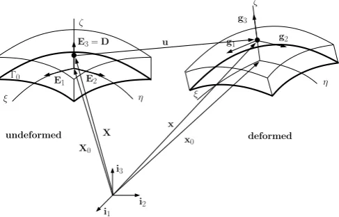
Figure1shows the continuum shell element in the undeformed and the deformed configuration. The reference surface is denoted byΓ0. The variablesξandηare the local curvilinear coordinates in the two independent in-plane directions, andζis the local curvilinear coordinate in the thickness direction. The position of a material point in the undeformed configuration reads:

X(ξ, η, ζ) =X0(ξ, η) +ζD(ξ, η), 0≤ζ≤1 (1)

ζ

η η

ξ

E2 E₁

i₁ i₂ i₃

deformed undeformed

Γ0

ζ

g₂ g₃

ξ

x₀ x X

X0

u

E₃=D g₁

Figure 1. Geometry and kinematics of the shell in the undeformed and in the deformed configurations.

A local reference triad can be established in any material point, and the covariant base vectors are obtained as the partial derivatives of the position vectors with respect to the curvilinear coordinates

Θ Θ

Θ = [ξ, η, ζ]. Defining a set of basis vectors on the reference surface in the undeformed configuration as:

Eα=

∂X0

∂Θα , α= 1,2 (2)

the shell director reads:

E3=D=

E1×E2

||E1×E2||

t (3)

withtthe thickness of the shell. Using equation (1), the covariant triad is obtained as:

Gα=

∂X

∂Θα =Eα+ζD,α , α= 1,2

G3=D

(4)

where the subscript comma denotes partial differentiation.

The displacement field u can be of any order, and, in the deformed configuration, the covariant triad reads:

g_i= ∂x

∂Θi =Gi+u,i , i= 1,2,3 (5)

Using equations (4) and (5) the metric tensors G and g become:

Gij =Gi·Gj , gij=gi·gj , i, j= 1,2,3 (6)

The contravariant basis vectors can be derived as:

Gi = (G)−1

Gi (7)

with(G)−1

the inverse of the metric tensor with componentsGij.

The Green-Lagrange strain tensorγ is defined conventionally in terms of deformation gradient

F:

γ= 1 2(F

T

·F−I) (8)

with I the unit tensor. The deformation gradient can be written in terms of the base vectors as:

F=g_i⊗Gi (9)

which leads to following representation of the Green-Lagrange strain tensor:

γ=γijGi⊗Gj with γij =

1

2(gij−Gij) (10)

where the summation convention has been used for repeated indices. Substituting equations (4) and (5) forGijandgij yields:

γij =

1

2(Gi·u,j+u,i·Gj+u,i·u,j) (11)

As stated in the Introduction, stresses are computed using a three-dimensional constitutive relation in a continuum shell formulation. Assuming small strains, a linear relation between the rates of the Second Piola-Kirchhoff stress tensor S and the Green-Lagrange strain tensor can be adopted:

DS=C_{:Dγ (12)}

whereC_{is the material tangential stiffness matrix.}

Using a Total Lagrangian formulation the internal virtual work is expressed in the reference configurationΩ0as:

δWint =

Z

Ω0

δγ:SdΩ0 (13)

The resulting system of non-linear equations is solved in an incremental-iterative manner. When using a Newton method for the iterative solutions, the formation of the tangential stiffness matrix is necessary, which is obtained by linearising the internal virtual work, equation (13):

D(δWint) =

Z

Ω0

(δγ:DS + D(δγ) :S)dΩ0 (14)

with the virtual strainδγandD(δγ)defined as:

δγij =

1

2(gi·δu,j+δu,i·gj) (15)

and

D(δγij) =

1

2(D(u,i)·δu,j+δu,i· D(u,j)) (16)

3. ISOGEOMETRIC FINITE ELEMENT DISCRETISATION

In this section we briefly recapitulate basic concepts of isogeometric analysis, including the B´ezier extraction technique, as well as some issues regarding its finite element like implementation.

3.1. Fundamentals of NURBS and B-splines

A B-spline is a piecewise polynomial curve composed of a linear combination of B-spline basis functions:

C(ξ) =

n

X

i=1

Ni,p(ξ)Pi (17)

wherepis the order andnis the number of the basis functions. TheNi,p(ξ)represents a B-spline

basis function and the coefficientsPiare points in space, referred to as control points. B-splines are

defined over a knot vector,ΞΞΞ, which is a set of non-decreasing real numbers representing coordinates in the parameter domain:

ΞΞΞ = [ξ1, ξ2, ..., ξn+p+1]

continuity while it reduces toCp−1

across a knot. If a knot value appearsktimes, the knot is called a multiple knot. At this knot the continuity is Cp−k_{. A B-spline is said to be open if its first and}

last knots appearp+ 1times. For the exact definition of univariate B-splines we refer to [22,23]. Two-dimensional (bivariate) splines are obtained as a tensor product. As a generalisation of B-splines, NURBS are now commonly used in Computer Aided Design (CAD) packages. They are obtained by augmenting a control point with a weightWi>0, so that the NURBS basis functions

are obtained as:

Sα,p=

Nα,p(ξ)Wα

W(ξ) (18)

where W(ξ) =Pn

i=1Ni,p(ξ)Wi is the weighting function, and no summation implied over the repeated index α. In two dimensions, NURBS surfaces are constructed by the weighted tensor product of B-spline functions.

In order to blend isogeometric analysis into existing finite element computer programs, B´ezier elements and B´ezier extraction operators have been proposed to provide a finite element structure for B-splines, NURBS and T-splines [24, 25]. A degree p B´ezier curve is defined by a linear combination of p+ 1 Bernstein basis functions B(ξ) [26]. Similar to B-splines, by having an appropriate set of control points, a B´ezier curve is written as:

C(ξ) =PTB (19)

A B´ezier extraction operator maps a piecewise Bernstein polynomial basis onto a B-spline basis:

N(ξ) =CB(ξ) (20)

This transformation makes it possible to use B´ezier elements as the finite element representation of B-splines or NURBS. The extraction operator is obtained by means of knot insertion. The reader is referred to Refs [24,25] for more details on the calculation of the extraction operator.

3.2. Isogeometric finite element implementation

As argued in [20] the total displacement field of the shell can be discretised as:

u(ξ, η, ζ) =

ncp

X

I=1

NI(ξ, η, ζ)aI (21)

where aIare the displacement degrees of freedom. We assume thatnandmare the number of shape

functions (or the control points) in the reference surface and in the thickness direction, respectively (ncp=n×m). Hence, the shape functionsNIread:

NI(ξ, η, ζ) =Si(ξ, η)Hj(ζ),

I=i+ (j−1)n,

i∈ {1, ..., n} , j∈ {1, ..., m}.

(22)

where Si(ξ, η) is the basis function from the B´ezier element in the reference plane and Hj(ζ)

is the B-spline function in the thickness direction. This equation implies that the trivariate basis functions NI are decomposed into a surface part and a thickness part which can have different

orders of interpolation,psandph, respectively. The strains are subsequently computed from these

displacements using shell kinematics, see Section 2.

As we only model a surface of the shell rather than the complete geometry, it is assumed that every control point on the reference surface has 3×mdegrees of freedom, where mis the number of control points in the thickness direction. Therefore, in a B´ezier mesh each control pointPicontains

a vector of degrees of freedomΦi, as follows:

Φi= [a1x, a1y, a1z, ..., axm, amy, amz]T , i= 1,2, ..., n (23)

whereax,ay,az denote the displacement components. Furthermore, by combining equations (21)

and (22) the displacement components can be written as follows:

uk(ξ, η, ζ) = m

X

j=1

n

X

i=1

aji_kSi(ξ, η)Hj(ζ) (24)

where the subscriptkrefers to the 1, 2, 3 (orx, y, z) directions.

The virtual strain vector, cf. equation (15), can be related to the control points degrees of freedom as:

δγ=B¯δΦ (25)

It is noted that the virtual strain vector and the correspondingB¯matrix in equation (25) are expressed in the non-orthonormal curvilinear base vectors. They must be transformed to the element local frame. The transformed matrix is represented by BL, see [20] for details.

3.3. In-surface and out-of-surface integration

The basis functions are defined over a parametric knot span, i.e (ξ, η, ζ)∈[0,1]3_{. In order to} carry out the numerical integration the basis functions and their derivatives should be calculated locally at quadrature points defined over a parent element, i.e ( ˜ξ,η,˜ ζ)˜ ∈[−1,1]3

. Moreover, the corresponding Jacobian determinant of the mapping must be calculated. The mapping for all the parametric coordinates is the same. For example, for a thickness element of[ζk, ζk+1]the mapping is:

ζ=ζk+ (˜ζ+ 1)

ζk+1−ζk

2 (26)

withζ˜the parent element coordinate. The kinematic parameters in terms of B-spline and NURBS parametric coordinate must be written in the right format. To this end, equation (4) is rewritten as:

Gα=

∂X

∂Θα˜ =Eα˜+

ζk+ (˜ζ+ 1)

ζk+1−ζk

2

D,α˜ , α˜= 1,2

G3= ∂X

∂ζ˜ =

ζk+1−ζk

2 D

(27)

As we employ independent discretisations for the reference surface of the shell and for the thickness direction, the numerical integration schemes in the in-plane and out-of-plane directions are also decoupled. Accordingly, the B´ezier extraction operator will be used for the integration over the surface. First, the geometry of the reference surface is mapped to its corresponding NURBS parametric space(ξ, η)∈[0,1]2_{. Then, the second mapping is carried out to the B´ezier space where} the parent element( ˜ξ,η)˜ ∈[−1,1]2_{and the extraction operator are obtained.}

Through-the-thickness integration is done by using a connectivity (or IEN) array. Using this array we determine which functions have a support in a given element. Assume that we use a quadratic B-spline defined over a knot vector ofT = [0,0,0,1

2,1,1,1]. This definition leads to two elements of [0,1

2]and[ 1

2,1]over the thickness and four global basis functions. Each element supportsph+ 1 = 3 basis functions of the global basis. The IEN array is:

[IEN]ne×ph+1=

1 2 3 2 3 4

2×3

(28)

The assembly of the element stiffness matrices is done according to the shared basis functions (number 2 and 3 in this case).

3.4. Modelling weak and strong discontinuities in the displacement field

Since B-spline and NURBS basis functions areCp−k _{continuous at a knot with multiplicitykthe}

C

ζ

C

ζ Hi

0

0.5 1

0

1 T = [0,0,0, 1 2,1,1,1]

ζ 0

0.5 1

0

1 T = [0,0,0, 1 2,

1 2,

1 2,1,1,1]

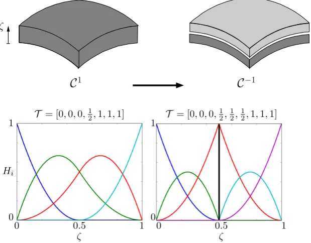
Figure 2. Introducing a strong discontinuity in the thickness direction of a shell.

Figure2shows the steps needed to introduce a discontinuity in the thickness direction. In this figure it is assumed that a quadratic B-spline defined over a knot vectorT = [0,0,0,1

2,1,1,1]has been used in the thickness direction of the shell. This results in four basis functions,Hi, which areC1

continuous atζ=1

2. A complete separation of the layers is obtained by inserting two knots to arrive at:_T = [0,0,0,1

2, 1 2,

1

2,1,1,1]. Figure2shows the corresponding basis functions through the knot insertion process.

It is important to note that if this method to introduce strong discontinuities is adopted in the construction of a single volumetric B-spline or NURBS patch, the inserted discontinuity will have a global influence, i.e. it will propagate throughout the patch. While this is not a problem for when weak discontinuities are inserted to model layers, it can be restrictive when used to model delamination by means of strong discontinuities. This restriction can be removed by adopting a localised definition of the basis functions, see also [21]. Alternatively, linear constraints can be used to represent partially delaminated patches [20].

4. COHESIVE INTERFACE FORMULATION

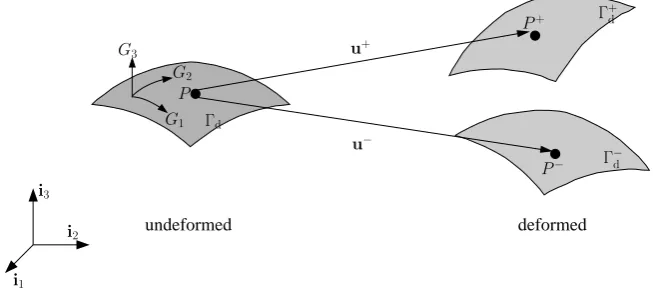
In this study delamination is modeled by applying a cohesive relation between the layers. Figure3

shows the undeformed and deformed configurations of a cohesive surface. It is noted that the undeformed cohesive surfaceΓdis calculated using equation (1) based on the the reference surface

Γ0in Figure1, which was used to construct the continuum shell element.

The virtual work of the cohesive tractionstmust be taken into account in the expression of the internal virtual work, which now becomes:

δWint=

Z

Ω0

δγγγ:SdΩ0+

Z

Γd

δv_·tddΓd (29)

withvthe displacement jump between the two layers. The latter quantity is defined as (Figure3):

v(ξ, η) =u+(ξ, η)−u−(ξ, η) (30)

with u+_{and u}−_{the displacement vectors of the material pointsP}+_andP−_{with respect to the global}

coordinate system, respectively. Defining the traction at the discontinuity as td= [tn,ts2,ts3]

T

deformed undeformed

G1

G2

u−

Γd

u+

P+

P−

i3

i1

i2

Γ− d

Γ+ d

P G3

Figure 3. Deformation of the interface.

with a normal component denoted by the subscriptnand two shear components, denoted by the subscriptss2ands3, respectively, its rate,Dtd, is related to the rate of the displacement jumpDvd

at the discontinuity by:

Dtd =TdDvd (31)

with Td as the tangent stiffness of the interface. Inserting the constitutive relation (31) into the

expression of virtual work in equation (29) requires a transformation from the local frame of the discontinuity surface (n,s2,s3) to the global frame of reference (i1,i2,i3). Denoting the rotation matrix as Q we have:

Dt=QT_Dtd=QTTdDvd =QTTdQDv (32)

and the tangent stiffness in the global reference frame is given by:

T=QTTdQ (33)

The displacement jump v can be expressed in terms of the displacements of the control points as:

v(ξ, η) =H(ξ, η)a (34)

with:

H=





−S1 0 0 · · · −Sn 0 0 S1 0 0 · · · Sn 0 0

0 −S1 0 · · · 0 −Sn 0 0 S1 0 · · · 0 Sn 0

0 0 −S1 · · · 0 0 −Sn 0 0 S1 · · · 0 0 Sn





(35) where_{Si}n1 are the basis function defined over the reference surface in equation (22) and:

aT=

a1−

x a1y− a1z− · · · axn− any− anz− ax1+ a1+y a1+z · · · axn+ any+ anz+

(36) as a vector containing the displacement degrees of freedom on the top and bottom surface of the interface. The internal force vector now reads:

fint=

Z

Ω0

BT_LSdΩ0+

Z

Γd

HTtddΓd (37)

where the areadΓdis calculated from:

dΓd =

√

G33p_{det(G) dξdη (38)}

withG33_=G3

·G3, and G3obtained from equation (7). The stiffness matrix is derived in a standard manner as:

with the material and geometric parts defined as, see also [20]:

Kmat=

Z

Ω0

BT_LC_{BLdΩ0 (40)}

and

Kgeom=

Z

Ω0

∂BT_L

∂ΦSdΩ0 (41)

while the additional term that stems from the cohesive tractions at the interface reads:

Kint=

Z

Γd

HTTHdΓ =

Z

Γd

HTQTTdQHdΓd (42)

4.1. Calculation of the rotation matrix

To calculate the rotation matrix, we first must compute the triad (n,s2,s3) on the discontinuity surface. This triad is assumed to be the average of the covariant base vectors on the top surfaceΓ+

d

and the bottom surfaceΓ−_d:

n=1 2(g

+ 3 +g

−

3)

s2=1₂(g+1 +g

−

1)

s3=1₂(g+2 +g

−

2)

(43)

It is noted that the the covariant base vectors (g1,g2,g3) are in the deformed configuration and are calculated based on the undeformed triad (G1,G2,G3) using equation (5), which gives:

g±_i = ∂x

∂Θi =Gi+u ±

,i , i= 1,2,3 (44)

Based on equation (4) the required Ei terms for the calculation of Gi can be determined. For the

calculation of u±_,i in (44) we also need the derivatives of the basis function defined on the reference surfaces. As an example we have:

u±_,i =





S1,i 0 0 · · · Sn,i 0 0

0 S1,i 0 · · · 0 Sn,i 0

0 0 S1,i · · · 0 0 Sn,i

           

a1± x

a1± y

a1± z

.. .

an± x

an± y

an± z           (45)

With the triad (n,s2,s3) on the discontinuity surface we can determine the rotation matrix:

Q=





cos(i1,n) cos(i1,s2) cos(i1,s3) cos(i2,n) cos(i2,s2) cos(i2,s3) cos(i3,n) cos(i3,s2) cos(i3,s3)



 (46)

withcos(a,b) = a·b

|a_{| |}b_|.

4.2. A mixed mode constitutive model for the interface

The propagation criteria under mixed-mode loading is based on the dissipated energy and the fracture toughness [29,30]. Delamination propagates when the dissipated energy equals or exceeds the fracture toughness. The expression for the critical energy release rate reads:

Gc=GIc+ (GIIc− GIc)Bη whereB= Gs

GT

(47)

where for a certain mode ratio,Gsis the dissipated energy in shear, andGT is the total dissipated

energy. The parameterηis obtained from experimental data, e.g. from mixed-mode bending tests. The initiation criterion can be written as:

(t0)2= (t0n)

2 + ((t0s)

2

−(t0n)

2

)Bη (48)

where n refers to normal opening, and s to sliding. The initiation and propagation criteria will be used to obtain the onset displacement jump and final displacement jump used in a damage evolution law. Under mixed-mode loadings, the damage evolution law is related to the norm of the displacement jump of the interface. This equivalent displacement jump is defined as:

λ=phvni2+vs2 (49)

withh.ithe MacAuley brackets, defined ashxi= 1

2(x+|x|).vnis the displacement jump in mode I andvsis defined as:

vs=

q

v2 2+v

2

3 (50)

wherev2andv3refer to the displacement jumps in mode-II and mode-III, respectively.

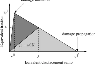
Equivalent traction

damage propagation damage initiation

Eqivalent displacement jump t

t0

vf

λ

v0

(1−ω)K

Figure 4. Linear softening law for the delamination model.

Damage is initiated when the equivalent displacementλexceeds a threshold or initial value. This initiation value can be formulated in terms of displacements similar to the initiation criterion (48) as:

(v0₎2_{= (v}0

n)

2_{+ (v}0

s)

2

−(v0

n)

2

Bη ₍₅₁₎

Assuming that the area under the traction-displacement jump curve in Figure 4 is equal to the fracture toughness, the final displacement jump which corresponds to full opening of the delamination crack is obtained as:

vf ₌ 2Gc

Kv0 (52)

withKthe initial stiffness of interface.

The constitutive law relates the cohesive traction ti to the displacement jump vi in the local

coordinate system and reads:

ti= (1−ω)Tijvj−ωTijvnjh−vni, i, j =n, s2, s3 (53)

withω as the damage variable. The stiffness tensorTij is defined asTij =δijKpwhereδij is the

Kronecker delta andKpis a penalty stiffness. In (53) the penetration of the two opposite layers after

complete decohesion is avoided by the last term by using the MacAuley brackets. In the constitutive relation (53) the damage parameterω reflects the decrease of the stiffness of the interface after the onset of damage. For a certain equivalent displacement jump the damage derives from:

ω=min{v

f_(λ−v0₎

5. NUMERICAL SIMULATIONS

The isogeometric continuum shell formulation is now verified and assessed through different examples. In Table I. We distinguish between two cases for the isogeometric continuum shell element (CSIGA): (i) without _C0 _{planes between the layers (lumped), and (ii) with}

C−1 _planes to simulate static delamination (discontinuous). Different orders of interpolation can be used in the plane as well as in the out-of-plane direction for each case. For instance, in the remainder ”lumped(3,2)” will denote a CSIGA element without_C0 _{(weak discontinuity) planes between the} layers, with a third-order NURBS/T-spline interpolation in the plane, and a second-order B-spline in the thickness direction.

Table I. Nomenclature of solid-like and continuum shell elements.

Model In-plane discretisation Out-of-plane discretisation SLS [6] 1st

or2nd

order Lagrange 1st

order Lagrange CSIGA(p, q)

lumped pth_{order NURBS / T-Spline q}th_{order B-Spline}

discontinuous pth_{order NURBS / T-Spline q}th _{order B-Spline with one}

C−1 continuity to represent a delamination. The other interfaces are_C0_continuous.

5.1. Locking

In this section we investigate shear locking and membrane locking which can occur when decreasing the thickness of shell elements. A clamped plate and a cylindrical shell, both under bending loads are used to assess the locking phenomenon.

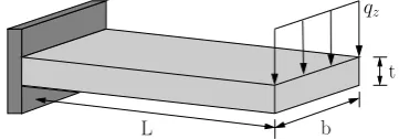
5.1.1. Shear locking Figure5shows the geometry of a plate subject to bending [7]. The plate has a Young’s modulus E= 1.08

Pa and a Poisson’s ratio ν= 0.3. The dimensions of the plate are:

L= 10m,b= 1m and the thicknesstvaries through the test. The plate is fully clamped at one end and a transverse loadqz= 100t3Nm2is applied at the other end.

L b

t qz

Figure 5. Geometry of the clamped plate under bending.

As a reference value we consider the displacement at the free end according to the beam theory,

δ=P L3_{/3EI which results inδ= 0.004m for this test. The numerical simulation is done with} two meshes of 64 CSIGA lumped(2,2) and 64 CSIGA lumped(3,2) elements. Figure 6shows the obtained normalised displacements for different ratios of L/t. It is clear that employing second order and third-order NURBS basis functions for the in-plane discretisation result in a behaviour that is insensitive to shear locking also when the thickness of the plate is reduced.

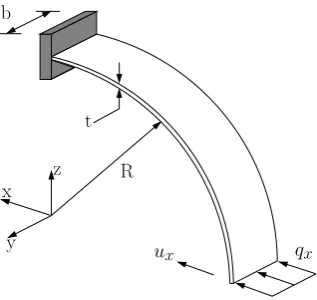
5.1.2. Membrane locking Membrane locking can occur in curved structures [17,18]. Therefore, a cylindrical shell as shown in Figure7is modelled. The shell has a radius ofR= 10m and a width of

b= 1m. Young’s modulus and Poisson’s ratio are1000Pa andν = 0respectively. The cylindrical shell is clamped at one edge and subjected to a constant distributed load of qx= 0.1t3Nm2. An

analytical solution based on the Bernoulli beam theory gives a value of approximately0.942for the radial displacement.

0.8 0.85 0.9 0.95 1 1.05 1.1 1.15 1.2

0 50 100 150 200 250 300 350 400

R

ela

tiv

e

d

is

p

la

ce

m

en

t

Ratio length to thickness, L/t 64 lumped(2,2) 64 lumped(3,2)

Figure 6. Normalised displacement of the plate under bending obtained for different ratios of L/t.

qx

t b

ux

x

z R

y

Figure 7. Geometry of the cylindrical shell

The numerical results for various meshes and thicknesses are presented in Figure8. In the figure, the mesh size shows the number of elements in the radial direction, while only one element has been used in the width direction. According to the results, a low number of elements of order two, 16 CSIGA lumped(2,2) elements, exhibit membrane locking. Keeping the NURBS order fixed and increasing the number of elements to 64 removes locking. Employing 16 third-order NURBS elements the results are insensitive to locking as well.

0.2 0.3 0.4 0.5 0.6 0.7 0.8 0.9 1 1.1

0 100 200 300 400 500 600 700

R

a

d

ia

l

d

is

p

la

ce

m

en

t,

ux

Slenderness R/t 16 lumped(2,2)

64 lumped(2,2) Bernoulli 16 lumped(3,2)

5.2. Mode I delamination

In this example mode I delamination (DCB test) is simulated. For this purpose an isotropic panel consisting of two layers is selected. The material properties of the layers are: a Young’s modulus

E= 1.0×1012 _{Pa and a Poisson’s ratio ν = 0.3. The geometry of the specimen is shown in} Figure 9. The specimen used for this simulation has a length L= 10m, a width b= 1m and a thickness 2h= 0.05m. An initial delamination with a length ofa0= 2.5m is placed between the two layers. The interface behaviour is captured by the exponential cohesive law proposed in [27]. The cohesive parameters are the fracture toughnessGc= 1KJ/m2and the maximum normal traction

tn ,max= 500Pa.

y

x

2h= 0.05m

z

a_{0 = 2}.5m L= 10m

b= 1m

qz

qz

Figure 9. Geometry of the panel with initial delamination

For this DCB test the relation between the applied load and the opening displacement can be obtained using linear elastic fracture mechanics (LEFM). Following the ASTM standard [28], the applied load in a DCB test for self-similar crack propagation is obtained as:

Fapplied=

r

GICb2h3E

12a2 (55)

with bandhthe width and the height of the specimen, respectively, Figure9, and whereais the crack length. The corresponding opening displacement is obtained as:

u=Fapplied 8a3

bh3_E (56)

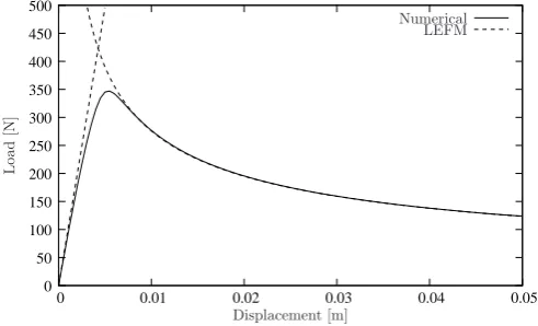
A numerical simulation has been carried out for a mesh containing 256×4 discontinuous CSIGA(2,2) elements and using the dissipation-based arc-length method proposed in [31], see also [32]. With this element delamination is modelled between the two layers where the delamination will propagate. Figure 10shows the numerical results, as well as the comparison with the LEFM solution. In the pre-peak regime there is an increasing difference between the linear-elastic solution and the non-linear solution because of energy dissipation in the latter solution. After the peak load has been reached the numerical results are in very good agreement with those from the calculations using linear elastic fracture mechanics, in particular for progressive delamination.

The deformation of the interface is also shown in Figure11, where the magnitude of the tractions is also indicated. To obtain a better insight into the interface behaviour, the traction magnitudes along the longitudinal axisxare monitored in Figure12. In both Figures11and12a maximum normal traction of500Pa has been obtained. It is clear that the traction oscillations persist, as in standard cohesive interface element models. A picture of gradual delamination propagation is presented in Figure13.

5.3. Buckling-delamination

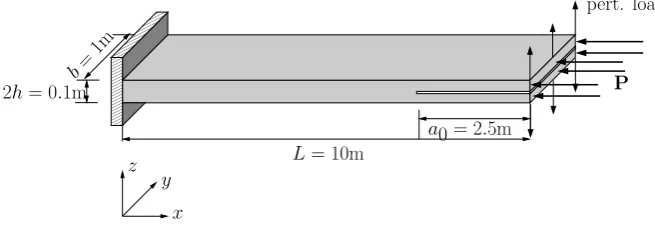
The next example concerns the two-layered panel of Figure14. It has a lengthL= 10m, a width

b= 1m, and a thickness2h= 0.1m. An initial delamination with a lengtha0= 2.5m is assumed. The material properties of the layers are: a Young’s modulusE= 2.0×108

Pa and a Poisson’s

0 50 100 150 200 250 300 350 400 450 500

0 0.01 0.02 0.03 0.04 0.05

L

o

a

d

[N

]

Displacement [m]

Numerical LEFM

Figure 10. Load-displacement curve of the mode-I delamination test.

Figure 11. Deformation of the interface in mode-I delamination.

−1200 −1000 −800 −600 −400 −200 0 200 400 600

0 1 2 3 4 5 6 7 8 9 10

T

ra

ct

io

n

,

t3

[N

/

m

2]

x [m]

Figure 12. Interface tractions along thex-axis of the mode-I delamination test specimen.

ratioν = 0.3. The panel is loaded by two compressive forcesP and small perturbations are applied to trigger the buckling mode. Again, an exponential cohesive law is considered at the interface with the following properties: fracture toughnessGc= 1KJ/m2and a maximum normal traction

tn ,max= 300Pa.

The test case shows a combination of two different non-linear mechanisms. First, the compressive load results in local buckling of the initially delaminated plies, which leads to an increase of the normal traction at the interface. Consequently, delamination growth will start when the normal traction reaches the ultimate traction of the interface. The numerical simulation has been done using a mesh of 512×4 discontinuous CSIGA(2,2) elements. The results are shown in Figure15. The graphs show the axial displacementux and the normal (out-of-plane) displacementuz versus the

Figure 13. Interface tractions during delamination propagation. The plots are for an out-of-plane displacement of0_.01_,0_.02_,0_.03_,0_.04_and0_.05_{, respectively, from top to bottom.}

00 00 00 00 00 00 00 00 00 00 00 00 11 11 11 11 11 11 11 11 11 11 11 11 000000 000000 000000 000000 000000 000000 000000 000000 000000 111111 111111 111111 111111 111111 111111 111111 111111 111111 y z

a_{0 = 2}.5m L= 10m

P pert. load

2h= 0.1mb =1m

x

Figure 14. Geometry of a panel under axial load with an initial delamination.

0 100 200 300 400 500 600 700 800 900

0 0.005 0.01 0.015 0.02 0.025 0.03 0.035 0.04 0.045

L o a d [N ]

Displacement,ux[m]

Numerical Analytical 0 100 200 300 400 500 600 700 800 900

0 0.1 0.2 0.3 0.4 0.5 0.6 0.7 0.8 0.9

L o a d [N ]

Displacement,uz[m]

Numerical Analytical

Figure 15. Load-displacement curves for the buckling-delamination test. (left): Load vs axial displacament. (right): Load vs out-of-plane displacement.

loads. The buckling loads are obtained using Euler beam theory as:

Fcr=

π2_Eh3 48a2

0

(57)

The critical buckling loads for the two extreme cases of a0= 2.5 m (initial delamination length) and of a0=L (fully delaminated panel) are821.63N and 51.35 N, respectively. It can be seen that the upper buckling load is lower than the analytical value. This difference is a matter of

Figure 16. Deformation of the interface in the delamination-buckling test.

choosing an appropriate perturbation load and also the maximum normal traction at the interface. For a lower perturbation load and higher maximum normal traction the numerical buckling load can be improved. This issue is clear from the agreement between the numerical buckling load and the analytical solution for the lower buckling load, where the perturbation load and the maximum normal traction do not influence the results.

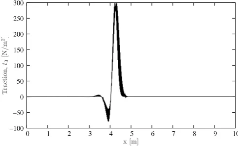
−100 −50 0 50 100 150 200 250 300

0 1 2 3 4 5 6 7 8 9 10

T

ra

ct

io

n

,

t3

[N

/

m

2]

x [m]

Figure 17. Interface tractions along thex-axis of the buckling-delamination test specimen.

Figure 16 presents the deformation of the interface for this test. Figure 17 shows the traction profile along the longitudinal axisx. In both cases a maximum normal traction of300Pa has been obtained as is in agreement with the material property of the interface. Again, traction oscillations are observed. The gradual delamination propagation has been visualised in Figure18, which shows the initiation of delamination and some further steps of the propagation process.

5.4. Mixed mode delamination of a curved panel

In this example delamination propagation is simulated in a curved panel. The geometry of the panel is shown in Figure19. The panel has a radius ofR= 10m, a width ofb= 1m and a thickness of t= 0.1m. The panel in considered to have two isotropic layers with a Young’s modulus and a Poisson’s ratio of2×108 _{Pa andν = 0.3, respectively. An initial delamination is taken over an} angle π₈. The curved panel is clamped at one edge and subjected to a constant distributed load ofqx.

This provides a suitable test case to investigate mixed-mode delamination propagation with large rotations at the interface. The mixed mode interface model discussed in Section4.2is used in this example. The material properties of the interface are:GIc= 10J/m2,GIIc= 10J/m2,K= 106Pa,

t0

3= 100Pa,t0s= 500Pa andη= 1.0.

The numerical simulations have been done using two different meshes of 256×1 and512×4

Figure 18. Interface tractions during delamination propagation of buckling-delamination test. The colors show the traction magnitude. The plots are for an axial displacement of 0_.05_,0_.1_,0_.2_,0_.3 _and 0_.4_,

respectively, from top to bottom.

qx

t b

ux

x

z R

y

Figure 19. Geometry of the curved panel with two layers and an initial delamination.

0 10 20 30 40 50 60

0 0.5 1 1.5 2 2.5 3 3.5 4

L

o

a

d

[N

]

Displacement,ux[m] 512×4

256×1

Figure 20. Load-displacement curve for delamination propagation in the curved panel.

Figure 21 shows the deformation of the panel. First, both layers start moving in the loading direction. In this process damage at the interface starts to grow. After a certain deformation and a certain damage growth, the lower layer moves in the reverse direction while the top layer keeps moving in the loading direction. At the final stage, the lower layer has returned to its initial configuration, the interface is fully damaged and the upper layer remains in the new configuration.

Figure 21. Deformation of the curved panel. Gray indicates the initial configuration, red represents the areas withω≈1_{and blue shows the areas withω}= 0_.

In Figure21, the gray colour indicates the initial configuration, the red colour represents the areas withω≈1and the blue colour show the areas withω= 0.

6. CONCLUDING REMARKS

Isogeometric analysis can be conceived as a novel finite element technology which, among other advantages, offers the possibility to capture the geometry of shells very accurately. Since the structural behaviour of shells can be highly sensitive to imperfections, and therefore to the precise geometric modelling of the shell, the use of splines in isogeometric analysis offers significant advantages. In a series of papers the authors have developed an isogeometric continuum shell element which models the shell surface exactly, and is capable of modelling weak and strong discontinuities in the shell [19,20]. A weak discontinuity occurs in a laminated shell between two bonded plies, while delamination converts this weak discontinuity into a strong discontinuity.

In Ref. [20] a B-spline has been introduced for the interpolation in the thickness direction. Knot insertion then allows for a straightforward introduction of discontinuities: weak discontinuities by a single knot insertion, and strong discontinuities by a double knot insertion (both in case of a quadratic B-spline in the thickness direction). It was shown that the accuracy of the in-plane stresses for a layered (weakly discontinuous) shell is then vastly improved. Moreover, a proof of concept was given that the method can be used for modelling static delaminations, i.e. the analysis of surfaces that were pre-delaminated.

during delamination propagation are in keeping with those found in the literature. The same holds for the case where the beam is subjected to a compressive load in the axial direction of the beam, so that a combined failure mode of buckling and a propagating delamination is obtained. The final example of mixed-mode delamination propagation in a curved panel confirms the versatility of the approach for arbitrary loadings and structures.

ACKNOWLEDGEMENTS

Funding from the EU Seventh Framework Programme FP7/2007-2013 under grant agreement n0 213371 (MAAXIMUS, www.maaximus.eu) is gratefully acknowledged. The research of C.V. Verhoosel has been funded by the Netherlands Organisation for Scientific Research (NWO) under the VENI scheme.

REFERENCES

1. Allix O, Ladev`eze P. Interlaminar interface modelling for the prediction of delamination. Composite Structures 1992; 22: 235–242.

2. Schellekens JCJ, de Borst R. A nonlinear finite-element approach for the analysis of mode 1 free edge delamination in composites. International Journal of Solids and Structures 1993; 30: 1239–1253.

3. Schellekens JCJ, de Borst R. On the numerical integration of interface elements. International Journal for Numerical Methods in Engineering 1993; 36: 43–66.

4. Irzal F, Remmers JJC, Verhoosel CV, de Borst R. An isogeometric analysis B´ezier interface element for mechanical and poromechanical fracture problems. International Journal for Numerical Methods in Engineering 2014; 97: 608– 628.

5. Nguyen VP, Kerfriden P, Bordas SPA. Two- and three-dimensional isogeometric cohesive elements for composite delamination analysis. Composites: Part B, 2014: 60: 193–212.

6. Parisch H. A continuum-based shell theory for non-linear application. International Journal for Numerical Methods in Engineering 1995; 38: 1855-1883.

7. Hashagen F, de Borst R. Numerical assessment of delamination in fibre metal laminates. Computer Methods in Applied Mechanics and Engineering 2000; 185: 141-59.

8. Belytschko T, Black T. Elastic crack growth in finite elements with minimal remeshing. International Journal for Numerical Methods in Engineering 1999; 45: 601-620.

9. Mo¨es N, Dolbow J, Belytschko T. A finite element method for crack growth without remeshing. International Journal for Numerical Methods in Engineering 1999; 46: 131-150.

10. Remmers JJC, Wells GN, de Borst R. A solid-like shell element allowing for arbitrary delaminations. International Journal for Numerical Methods in Engineering 2003; 58: 2013-2040.

11. Hughes TJR, Cottrell J, Bazilevs Y. Isogeometric analysis: CAD, finite element, NURBS, exact geometry and mesh refinement. Computer Methods in Applied Mechanics and Engineering 2005; 194: 4135-4195.

12. Cottrell J, Hughes T.J.R, Bazilevs Y. Isogeometric Analysis: Toward Integration of CAD and FEA. John Wiley & Sons, Chichester, 2009.

13. Sederberg TW, Zheng J, Bakenov A, Nasri A. T-splines and T-NURCCs. ACM Transactions on Graphics 2003; 22:477-484.

14. Kiendl J, Bletzinger KU, Linhard J and W ¨uchner R. Isogeometric shell analysis with Kirchhoff-Love elements. Computer Methods in Applied Mechanics and Engineering 2009; 198: 3902-3914.

15. de Borst R, Crisfield MA, Remmers JJC, Verhoosel CV. Non-linear Finite Element Analysis of Solids and Structures, Wiley Series in Computational Mechanics, Second edition, 2012.

16. Benson DJ, Bazilevs Y, Hsu MC and Hughes TJR. Isogeometric shell analysis: The Reissner-Mindlin shell. Computer Methods in Applied Mechanics and Engineering 2010; 199: 276-289.

17. Bischoff M, Wall W, Bletzinger KU, Ramm E. Models and finite elements for thin-walled structures. In: Encyclopedia of Computational Mechanics, Eds. Stein E, de Borst R, Hughes TJR, Vol. 2, Chapter 3, pp. 59-137. Wiley: Chichester, 2004.

18. Echter R, Oesterle B, Bischoff M. A hierarchic family of isogeometric shell finite elements. Computer Methods in Applied Mechanics and Engineering 2013; 254: 170-180.

19. Hosseini S, Remmers JJC, Verhoosel CV, de Borst R. An isogeometric solid-like shell formulation for non-linear analysis. International Journal for Numerical Methods in Engineering 2013; 95: 238–256.

20. Hosseini S, Remmers JJC, Verhoosel CV, de Borst R. An isogeometric continuum shell element for non-linear analysis. Computer Methods in Applied Mechanics and Engineering 2014; 271: 1–22.

21. Verhoosel CV, Scott MA, de Borst R, Hughes TJR. An isogeometric approach to cohesive zone modeling. International Journal for Numerical Methods in Engineering 2011, 87(1-5), 336–360.

22. Cox MG. The numerical evaluation of B-splines. IMA Journal of Applied Mathematics 1972; 10: 134-149. 23. de Boor C. On calculating with B-splines. Journal of Approximation Theory 1972; 6: 50-62.

24. Borden MJ, Scott MA, Evans JA, Hughes TJR. Isogeometric finite element data structures based on B´ezier extraction. International Journal for Numerical Methods in Engineering 2011; 87: 15-47.

25. Scott M.A, Borden M.J, Verhoosel C.V, Sederberg T.W, Hughes T.J.R. Isogeometric finite element data structures based on B´ezier extraction of T-splines International Journal for Numerical Methods in Engineering 2011; 88: 126-156.

26. Piegl L, Tiller W. The NURBS Book, Second Edition. Springer-Verlag, New York, 1997.

27. Xu XP, Needleman, A. Numerical simulations of fast crack growth in brittle solids. Journal of the Mechanics and Physics of Solids 1994: 42, 1397-1434.

28. ASTM D5528 01(2007)e2. Standard test method for mode I interlaminar fracture toughness of unidirectional fiber-reinforced polymer matrix composites; 2007.

29. Camanho PP, Davila CG, de Moura MF. Numerical simulation of mixed-mode progressive delamination in composite materials. Journal of Composite Materials, 2003; 37: 1415–1438.

30. Turon A, Camanho PP, Costa J. A damage model for the simulation of delamination in advanced composites under variable-mode loading. Mechanics of Materials, 2006; 38: 1072–1089.

31. Verhoosel CV, Remmers JJC, Guti´errez MA. A dissipation-based arc-length method for robust simiulation of brittle and ductile failure. International Journal for Numerical Methods in Engineering, 2009; 77: 1290–1321.