This is a repository copy of Branch-point motion in architecturally complex polymers: estimation of hopping parameters from computer simulations and experiments.
White Rose Research Online URL for this paper: http://eprints.whiterose.ac.uk/78833/
Version: Accepted Version
Article:
Bǎov́, P, Lentzakis, H, Read, DJ et al. (3 more authors) (2014) Branch-point motion in architecturally complex polymers: estimation of hopping parameters from computer simulations and experiments. Macromolecules. ISSN 0024-9297
https://doi.org/10.1021/ma5003936
[email protected] https://eprints.whiterose.ac.uk/ Reuse
Unless indicated otherwise, fulltext items are protected by copyright with all rights reserved. The copyright exception in section 29 of the Copyright, Designs and Patents Act 1988 allows the making of a single copy solely for the purpose of non-commercial research or private study within the limits of fair dealing. The publisher or other rights-holder may allow further reproduction and re-use of this version - refer to the White Rose Research Online record for this item. Where records identify the publisher as the copyright holder, users can verify any specific terms of use on the publisher’s website.
Takedown
If you consider content in White Rose Research Online to be in breach of UK law, please notify us by
Branchpoint motion in architecturally complex
polymers:
estimation of hopping parameters from computer
simulations and experiments
Petra Baˇcová,
†Helen Lentzakis,
‡,¶Daniel J. Read,
§Angel J. Moreno,
∗,†,kDimitris
Vlassopoulos,
‡,¶and Chinmay Das
⊥Centro de Física de Materiales (CSIC, UPV/EHU) and Materials Physics Center MPC, Paseo
Manuel de Lardizabal 5, E-20018 San Sebastián, Spain, Foundation for Research and Technology
Hellas (FORTH), Institute of Electronic Structure & Laser, Heraklion, Crete 71110, Greece,
Univerisity of Crete, Department of Materials Science and Technology, Heraklion, Crete 71300,
Greece, Department of Applied Mathematics, University of Leeds, LS2 9JT Leeds, UK, Donostia
International Physics Center, Apartado 1072, 20080 San Sebastián, Spain, and School of Physics
and Astronomy, University of Leeds, Leeds LS2 9JT, United Kingdom
E-mail: [email protected]
Abstract
∗To whom correspondence should be addressed
†Centro de Física de Materiales (CSIC, UPV/EHU) and Materials Physics Center MPC, Paseo Manuel de
Lardiz-abal 5, E-20018 San Sebastián, Spain
‡Foundation for Research and Technology Hellas (FORTH), Institute of Electronic Structure & Laser, Heraklion,
Crete 71110, Greece
¶Univerisity of Crete, Department of Materials Science and Technology, Heraklion, Crete 71300, Greece §Department of Applied Mathematics, University of Leeds, LS2 9JT Leeds, UK
Relaxation of branched polymers under tube based models involve a parameter p2 char-acterizing the hop-size of relaxed side-arms. Depending on assumptions made in rheological
models (e.g. about the relevant tube diameter for branchpoint hops) p2had been set to values varying from 1 to 1/60 in the literature. From large-scale molecular dynamics simulations of
melts of entangled branched polymers of different architectures, and from experimental
rhe-ological data on a set of well-characterized comb polymers with many (∼30) side-arms, we
estimate the values of p2 under different assumptions in the hierarchical relaxation scheme. Both the simulations and the experiments show that including the backbone friction and
con-sidering hopping in the dilated tube provides the most consistent set of hopping parameters in
different architectures.
1
IntroductionOver the last years, experimental studies on branched polymers have gone hand in hand with
the-oretical work aiming to explain their exceptional viscoelastic properties.1–4 While the
viscoelas-ticity of linear chains is well described by the tube theory,5 entangled branched polymer melts
reveal a more complex dynamic behavior as a consequence of their complicated structure.6 All of
them include one branchpoint (in the case of stars) or more (H-polymers, combs, Cayley trees,
hy-perbranched etc.), which dramatically slow down the overall relaxation of the material. The slow
relaxation processes are reflected in the rheological spectrum, extending over several time decades,
and play an important role during industrial processing.7A correct implementation of the
branch-point dynamics in tube-based models seems to be essential for accurate theoretical predictions of
the rheological properties of these materials.
Molecular segments in the entanglement network of branched polymers relax hierarchically,
progressing from the outer to the inner parts of the molecule. The arms are retracted back and
for-ward along the tubes and their retraction becomes less favorable as the branchpoint is approached.8
This leads to an exponential distribution of the relaxation times along the arm, and to a progressive
inner segments do not experience the entanglements with the outer ones, which have relaxed at
much earlier time scales. As a result, the original tube becomes wider (‘dilated tube’) with time.
This mechanism is known as dynamic tube dilution (DTD).9,10 Once the arms are fully relaxed,
they act as sources of additional friction, i.e., as frictional ‘fat beads’. The branchpoint at these
time scales probes the space liberated by the removed constraints of the arm, and performs diffusive
steps (hops) along the tube contour with a diffusivity given by:
D= p 2a2
2τa
(1)
where τa is the longest relaxation time of the arm and a is the tube diameter. This may be the
original or the dilated one (see below). In the following the symbol a will be used for the dilated
tube. The original, undilated, tube diameter will be denoted as a0. In the case of asymmetric
structures (e.g., T- and Y-shaped stars, combs, etc), the branched architecture is reduced to an
effective linear chain containing the frictional beads representing the relaxed short arms. At this
point, the final stage of the relaxation is mediated by reptation of the backbone. In symmetric
structures (symmetric stars, Cayley trees...) reptation is not possible, and after retraction of the
main arms all stress is considered to be relaxed; hopping of the central branchpoint is the only
available mechanism for later motion.
The factor p2 in equation Eq. (1) is a dimensionless constant called the hopping parameter.
Thus, it is assumed that the typical hopping distance is p times the tube diameter, and that
hop-ping occurs every time the arm relaxes. Naively, it may be expected that p2is of the order of unity.
However, a series of investigations have suggested considerably smaller values in the case of
asym-metric T-shaped stars with weakly or moderately entangled short arms. This was first pointed out
by Frischknecht et al.11 They found that, in order to reproduce the experimental rheological data
with hierarchical tube-based models, the value of p2needed to be adjusted depending on the length
of the short arm. The values obtained in Ref.11 varied in the range 1/4≤p≤1/60. The smaller
corresponding diffusivity compared to the naive value for p2=1. Thus, the relaxed short arms
in the asymmetric stars caused much more drag than expected, even in the case of very weakly
entangled short arms. Chen and Larson analyzed, in combination with hierarchical models,
rhe-ological data of asymmetric stars with the same length of the short arm, but this being linked at
different positions along the backbone (forming T-shaped or Y-shaped stars).12 They described the
experimental data by using a fixed hopping parameter p2=1/12. We note that an alternative
tube-model approach, the time marching algorithm (TMA) uses p2=1 but invokes different molecular
assumptions which in essence (implicitly) require a different friction due to the branch point. So,
for example, in TMA, reptation is determined by considering the length of the primitive path of the
whole backbone (not only of the unrelaxed fraction of the backbone, as in the BoB3or hierarchical
models2).
Branchpoint motion has also been characterized in more complex branched architectures. McLeish
et al.13 found the value p2=1/12 to account well for rheological data of H-polymers.14 Further
experimental studies generalized the approach for H-polymers of Ref.13 to the case of comb
poly-mers. Daniels et al.15kept the value of the hopping parameter p2=1/12 and analyzed the possible
factors affecting the rheological spectra. They studied the change in the dynamics with
increas-ing number of arms in the comb structure. Some authors incorporated the effect of the different
length of the free backbone ends and side arms .16,17 As previously found for their star-like
coun-terparts,11,18 rheological experiments of comb polymers with short, weakly entangled, branches
revealed that these exerted a higher frictional drag than expected.19 Kirkwood et al. proposed to
solve this problem by fixing again the value p2=1/12 and using a different, effective entanglement
length for the branches.19
Further investigations have shown that reduced values of p2 ≪1 are universally found for
branched architectures with weakly entangled short side arms, the values being strongly dependent
on the arm length.20–22 On the other hand, recent studies on comb polymers using the TMA, have
kept the original value of the hopping parameter, p2=1, as already mentioned, and used a different
that the effects of architectural dispersity have been recently considered and analyzed.24–26
There have been only a few theoretical attempts to specify a priori the value of p2. Lee et
al.20,27extended hierarchical tube models to include branchpoint diffusion in a self-consistent way,
accounting for linear rheology of Y-shaped asymmetric stars, combs and pom-pom molecules. The
hopping parameter was identified as p2 =1/ZAR being independent of the specific architecture,
with ZAR the entanglement density of the unrelaxed backbone segments at the hopping events.
Some studies using slip-link simulations have focused on the nature of the branchpoint motion
itself. Shanbhag and Larson 28 suggested that the branchpoint diffusion is limited by the full
removal of the entanglements around the short arm. Masubuchi et al.29 examined the relaxation
mechanisms of the branchpoint and their contribution to the viscoelastic relaxation of asymmetric
stars. They observed that the more asymmetric the structure is, the more relevant the contribution
of branchpoint hopping becomes for the overall relaxation of the star.
The above review of the literature reveals that there are a very large range of values reported for
the hopping parameter p2. Why is this? We consider that there are two separate causes, as follows.
Firstly, there are different assumptions made about the branchpoint hopping process itself,
within the context of dynamic dilution theory. These assumptions are about two aspects of the
hopping: i) the length-scale associated with hops– this might be set by the original ("thin") tube
diameter or dilated ("fat") tube diameter, and ii) the direction, or path, of the hopping motion– hops
may be considered to occur along the paths of the thin tube contour or fat tube contour. Different
versions of hierarchical tube-based models make different choices on these two characteristics of
the branchpoint hopping motion.11,15–17,19,22,30
Secondly, the appropriate value of p2 is normally determined by inference from rheological
data, rather than by measuring the branchpoint motion directly. The data are interpreted by
mak-ing use of a suitable (hierarchical) rheological model. In addition to the above assumptions made
about the hopping process itself, such models encode further assumptions about polymer
relax-ation,3,4,31for example in the mathematical description of deep contour length fluctuations. See,
are themselves dependent on the model used to interpret the data. So, it is quite possible that this
process deduces the wrong rate of branchpoint diffusion (because the branchpoint motion is not
measured directly) which is then interpreted using the wrong assumptions for the hopping process.
It is therefore not surprising that a wide range of numerical values for p2ensue.
Given the wide range of assumptions on branchpoint hopping introduced by hierarchical
mod-els, we aim in this article to address a fundamental issue: can we rule out some of these
assump-tions? We present a critical analysis of the consistency of the different assumptions for branchpoint
hopping. We perform large-scale molecular dynamics (MD) simulations on several branched
ar-chitectures. These include symmetric stars, asymmetric T-shaped and Y-shaped stars, combs and
mixtures of stars and linear chains. The MD simulations allow us to analyze directly the diffusive
motion of the branchpoints, rather than make inferences from rheology data. We also analyze
fric-tion of the branchpoints and tube dilufric-tion. Using these data, we determine p2-values for each set
of specific assumptions for branchpoint hopping.
Since our aim is to rule out some of these assumptions, we state in advance our criterion for
deciding what is a “good” assumption, and what is a poor one. Our criterion is simple, and based
on the requirement of a universal behavior: a good set of assumptions should result in broadly
similar values of p2 across the different systems studied. So, if a specific assumption regarding
branchpoint hopping requires very different values of p2 to model the branchpoint diffusion of
different systems, then that particular assumption will be ruled out by this exercise. Then, having
arrived at an optimal set of assumptions, we can go on to ask what typical value of p2 should
be used. Throughout this exercise, we shall pay particular attention to errors in determining the
different physical quantities measured by the simulations. Where possible, we aim to estimate
quantities by more than one method, as a check on the consistency of our results. This allows us
to decide whether differences in the p2-values obtained for different simulations are significant, or
within reasonable error bounds.
As a final check on our conclusions, we discuss simulation results in comparison with
branches. This type of experimental system was chosen for several reasons: (i) the large number
of side arms means that there is a discernible experimental signal of the arm relaxation in the linear
rheology data, allowing an experimental estimate to be made of the arm relaxation time, and (ii)
following relaxation of the side arms, the combs are geometrically simple (linear) objects, and so
the terminal relaxation can be analyzed using reptation theory. Thus, while direct experimental
measurement of branchpoint motion is not possible we can at least make an estimate of the motion
without resorting to one of the more complicated hierarchical models. In what follows, we discuss
our analysis of the experimental system in parallel with the simulation results because there are
some similarities in the analysis, for example difficulties in estimating the arm relaxation time, and
the need to use several different methods as a check on consistency.
The article is organized as follows: in Section 2 we present the simulated systems of branched
polymers, we describe the simulated model and give simulation details. In Section 3 we summarize
the main theoretical predictions for branchpoint motion. This section introduces equations related
to branchpoint motion that are later used for obtaining p2 of the simulated and experimental
sys-tems. In Section 4 and Section 5 we estimate the variables figuring in the equations in Section 3
for different molecular architectures, by analyzing simulation and rheological data, respectively.
Subsequently, we use the obtained variables to calculate the values of p2 for both the simulated
and experimental systems. Results are summarized and discussed in Section 6. Conclusions are
given in Section 7.
2
Simulation detailsThe branched polymers in our MD simulations were modeled by the bead-spring Kremer-Grest
model.33 Monomeric units are coarse-grained into beads with diameterσ, mass m0 and excluded
volume represented by a repulsive Lennard-Jones (LJ) potential:
ULJ(r) =
4ε h
σ
r 12
− σr6
+1 4
i
for r≤rc,
0 for r>rc,
with cut-off distance rc=21/6σ. Bonded beads are connected by springs, introduced as a
finite-extension nonlinear elastic (FENE) potential:
UF=−
1 2KFR
2 Fln
" 1−
r RF
2#
, (3)
with spring constant KF =30ε/σ2 and maximum spring length RF =1.5σ. In addition to the
original Kremer-Grest interactions, we applied a bending potential given by:
Ubend(θ) =kθ(1−cosθ), (4)
whereθ is the angle between three consecutive beads (θ=0 for a rod). A bending constant kθ =2ε
was imposed to increase slightly the stiffness of the chains. The resulting characteristic ratio at the
simulated density and temperature (see below) is C∞=3.68. This choice was made to decrease
the value of the entanglement length in comparison to that of the flexible chains (kθ =0).34 In the
following we assume a nominal value of the entanglement length of Ne≈25. This value is the
average of NePP=23 and NeMSD=27, these being estimated by analysis of the primitive path35and
monomer mean square displacement,18 respectively. In the following we will use the diameterσ
as the length unit, and time will be expressed in units of τ0= (m0σ2/ε)1/2. The corresponding
entanglement timeτe for our model isτe=1800τ0.18
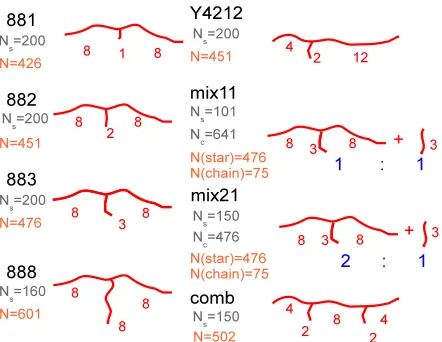
The simulated systems are illustrated in Figure 1. These include symmetric stars, T- and
Y-shaped asymmetric stars, combs, and mixtures of T-stars with linear chains. Red labels denote the
number of entanglements per arm in each architecture (by using the nominal value Ne=25 beads
per entanglement segment, as mentioned before). See figure caption for details. The simulated
architectures and used values for the arm lengths have been selected to investigate several effects
on the dynamics, namely: i) the effect of the short-arm length for a fixed architecture (881, 882,
883 and 888 systems), ii) the effect of the branchpoint position for stars with identical backbones
and short arms (882 and Y4212 systems), iii) the effect of adding an identical, short arm to an
with weakly entangled linear chains (883 vs. mix11 and mix21 systems).
All the systems were simulated, by using the ESPResSo package,36 at number density ρ =
0.85σ−3 and temperature T =ε/kB, with kB the Boltzmann constant. The number of beads in
the simulation box for the different investigated systems ranged from 75300 to 107100 (see details
in Figure 1). The polymers were first constructed by joining building blocks that were sampled
from simulations of unentangled stars and linear chains with the same interactions of Eq.
(2)-Eq. (4). The angles at the junction points between building blocks were chosen in order to obtain
the correct distribution of intramolecular distances (see Ref.37 for details). Once the polymers
were constructed and randomly inserted in the simulation box, we equilibrated the system. The
equilibration protocol, based on the method of Auhl et al.37 consisted of three steps: i) a Monte
Carlo run for prepacking of rigid macromolecules, ii) an MD run for progressive introduction of
excluded volume by capped LJ interactions (‘slow push-off’), and iii) a further equilibration MD
run with the full interactions. A detailed description of the protocol can be found in Ref.38 After
equilibration, production MD runs were performed, extending over typically one to five billion
MD steps. The MD runs were integrated by using the velocity-Verlet algorithm with time step
∆t=0.01τ0. The temperature in the MD runs was controlled by the Langevin thermostat with a
friction constantΓ=0.5m0/τ0.
3
Diffusion of the branchpoint: theoretical backgroundAfter the relaxation of the short arm, this effectively acts as a frictional ‘fat bead’. Consequently
the backbone, which in the case of the asymmetric stars is formed by the two long arms, is able to
reptate. The branch point motion at these time scales can be seen as a curvilinear diffusion along a
tube of diameter a. The trajectory of the branch point is assumed to be a random walk,
Figure 1: Schematic representation of the simulated systems. The numbers at each arm denote the number of entanglements in the arm, by using the nominal value of Ne=25 beads per entanglement
segment (see above). In the rest of the paper the different simulated systems will be denoted according to the big labels. The simulated systems include: i) asymmetric T-shaped stars (881, 882, 883), ii) asymmetric Y-shaped stars (Y4212), iii) symmetric stars (888), iv) comb polymers, and v) mixtures of 883-stars with linear chains. The fraction of beads in the simulation box that belong to the stars is 1/2 in the mixture ‘mix11’ and 2/3 in the mixture ‘mix21’. The labels 1:1 and 2:1 denote such relative compositions. Ns denote the total number of stars in the simulation box, Ncdenote the number of linear chains in the mixtures. N represents the total number of beads per
macromolecule.
wherehr2iis the mean square distance between the start and end points of the trajectory, and|L|is
the length of the primitive path that is explored by the branch point in this trajectory. A Gaussian
distribution is assumed for the diffusion length L. Therefore, Eq. (5) can be expressed as
hr2i=p 2a 2πhL2i
Z ∞
0
L exp
−L2
2hL2i
dL, (6)
which leads to the relation:
hr2i=a q
2hL2i/π. (7)
Since we have assumed a diffusive motion of the branch point along the primitive path, we can
relatehL2iand the diffusivity D as
where the factor 2 results from the one-dimensional character of the curvilinear diffusion. From Eq. (7)
and Eq. (8) we find:
D= π
4a2
hr2i
t1/2
2
. (9)
Eq. (9) provides a direct way of obtaining the diffusivity for the curvilinear, reptative motion of
the branchpoint. In the reptative regime the mean squared displacement will scale as5hr2i∝t1/2.
Therefore, by obtaining from the simulations the corresponding plateau value of the ratiohr2i/t1/2,
the diffusivity can be easily calculated. We note here that when dynamic tube dilution is included,
there are different tube diameters that could be considered. There are a set of nested tubes, each
of which is parameterised by its tube diameter, a. As written, Eq. (9) gives the effective diffusion
constant for the random motion of the branchpoint, when this motion is mapped onto the path for
the tube with diameter a. Thus a particular motion (giving rise to a plateau value ofhr2i/t1/2) can
be construed either as rapid diffusion along a tube path with a small tube diameter, or as slower
motion along a shorter tube path with a larger tube diameter.
As mentioned in the Introduction, the branchpoint is assumed to hop in the tube every time
the short arm relaxes ( Eq. (1)). This branchpoint hopping may occur in the skinny (a0) or in the
dilated (a) tube. In order to investigate both possible cases, we modify Eq. (1) in the way it was
done in eq. 11 of Ref.:3
D= p 2a4
h
2qτaa2
. (10)
The parameter ah denotes the tube diameter (a0 or a) in which the branchpoint hopping takes
place. In deriving Eq. (10), Ref.3 assumes that the length ah sets both (i) the typical distance of
the hops, and (ii) the tube contour along which the hops take place. This is then converted to an
effective diffusion constant D, for motion mapped on to the tube path set by tube diameter a. We
note that, if Eq. (9) and Eq. (10) are equated then the factor a2 cancels: the large scale motion
given by hr2i/t1/2 will depend only on the tube diameter ah within which hops take place. We
equate Eq. (9) and Eq. (10) below if we assume that branchpoint friction dominates the motion.
skinny tube) sometimes consider the length of the hop to be set by a0, but the path of the hop to be
along the dilated tube contour.
Eq. (10) includes an additional factor q. The factor q is the number of side arms attached to
the main backbone (q=1 for the stars, q=2 for the simulated combs), and it is introduced for
accounting for all frictional contributions from the relaxed q short arms. In the case ah=a and
q=1, Eq. (10) reduces to the original Eq. (1).
As mentioned in the Introduction, the hopping parameter p2 used in the expression for the
branchpoint diffusivity was experimentally found to be considerably smaller than unity, reflecting
a stronger drag from relaxed arms than expected. A possible explanation is that Eq. (1) and Eq. (10)
overestimate the diffusivity by missing the friction contribution from the chain itself. We attempt
to correct this point by adding the chain friction for the motion along the skinny tube, allowing for
a rescaling to the dilated tube in the manner of eq. 36 of Ref.39 The corresponding equation for the
diffusivity reads:
D=
3π2τeZ φαa2
0
+2qτaa 2
p2a4 h
−1
, (11)
where Z is the number of entanglements along the backbone, a0 is the undilated tube diameter,τe
is the entanglement time, andφα represents the fraction of material giving rise to slow constraints
(see below). As discussed in detail in Ref.39 (building on the earlier work of Viovy et. al40), the
factorφα in the first term on the right hand side of Eq. (11) arises because the ‘solvent’ (giving the
dilated tube) is actually formed by slow moving entangled chains. The fastest mode for diffusion
along the dilated tube is via chain motion along the skinny tube. Motion directly along the dilated
tube requires many constraint release events and is therefore much slower. The factorφα is due to
projecting chain motion along the skinny tube onto the shorter diluted tube path.
For the mixtures of asymmetric 883-stars (see Figure 1) and linear chains, constraint release
from the solvent (the short, linear chains) is a little faster, and we can refine equation Eq. (11) to
Ref.39):
D=
3π2τeZ
a2 0
"
φα+
2 3π2ντ
e
+ 1
1−φα
−1#−1
+2τaa
2
p2a4
h
−1
, (12)
where ν =cντs−1 is the constraint release rate from the linear chains in the mixture, τs is their
relaxation time and cν is the rate constant. In Eq. (12) we have dropped the factor q since for
the 883-stars q=1. We note that, in the limit of extremely fast constraint release (ν →∞) the
friction for chain motion along the dilated tube becomes independent ofφα. In practice, even for
the mixtures with short linear chains, Eq. (12) gives only a small correction to Eq. (11).
Again, we contrast Eq. (11) and Eq. (12) with the work of Frischknecht et al.11 When
con-sidering reptation of the backbone along the dilated tube, they assumed that the only friction
ex-perienced by the backbone was the monomeric (or “Rouse”) friction. This neglects the fact that,
for chain motion along the dilated tube, constraint release events need to occur, and these give rise
to drag on the chain. Here we consider two possibilities: that the constraint release events are so
slow, the fastest motion available to the chain is along the skinny tube, but subject to monomeric
friction - this gives Eq. (11). For the blends, we also consider including constraint release events
approximated to be at a fixed rate - this gives Eq. (12). The work of Frischknecht et al.
cor-responds to Eq. (12) in the limit ν →∞. Thus, in using Eq. (11) and Eq. (12), together with
hopping in a dilated tube, we are considering an option not used by Frischknecht et al., namely
branchpoint hopping in the dilated tube, but backbone motion dominated by movement along the
skinny tube. Finally, if we know the tube diameter and use the simulation value for the reptation
plateau inhr2i/t1/2, we can obtain the hopping parameter p2 by combining Eq. (9) with one of
the Eq. (10), Eq. (11), Eq. (12).
Once we have presented equations for branchpoint motion in the simulated systems, we draw
our attention to experiments. We will focus on the illustrative case of experimental comb polymers.
Regarding the analysis of the experimental combs, we have no direct access to the diffusivity D.
Therefore, we proceed in a related but different manner to obtain p2. As in the other asymmetric
short side arms. Likewise, reptation can be considered in a dilated tube (but with an enhanced
friction), due to the faster dynamics of the entanglements of the backbone with short side arms.
For each comb, we can deduce the number of effective entanglements, Zdil, in the dilated tube as:
Zdil=Zb Zb Zb+qZa
, (13)
where Zb and Za are the number of entanglements along the backbone and at each of the q side
arms, respectively. With this, the effective relaxation timeτe,dil of a diluted entanglement segment
can be obtained as:
τe,dil=τd/rdil, (14)
where τd is the experimentally measured terminal time of the comb, and rdil is the ratio of the
terminal to the entanglement time of the linear chain with the same number of entanglements, Zdil,
as the diluted comb. This ratio can be calculated from the Likhtman-McLeish theory for linear
chains as:41
rdil= τ lin d τlin
e
=3Zdil3 1−3.38 Z1dil/2
+4.17
Zdil
−1.55 Zdil3/2
!
. (15)
In applying Eq. (15) to combs, we are assuming that the combs behave exactly as rescaled linear
polymers in their terminal relaxation. In particular, we assume that the depth of contour length
fluctuations is commensurate with the diluted tube (c.f. the binary blend case in Ref.39). We also
assume that the rate of contour length fluctuations and terminal reptation are rescaled by exactly
the same time constant (i.e. slowed down compared to the corresponding linear chain by the large
contribution of side arm friction). Thus, the effective rescaled entanglement time τe,dil includes
contributions from side arm friction, just as the experimentally measured terminal timeτdincludes
the side arm friction. So, the diffusion constant we derive below ( Eq. (16)) is the effective diffusion
constant along the diluted tube, including contributions from the side arm friction.
For a linear chain, the entanglement time and curvilinear diffusivity are given respectively by
τe =ζNe2b2/(3π2kBT) and D=kBT/(ζZNe), where Ne is the total number of monomers per
Moreover a20=Neb2 due to Gaussianity. By combining the former expressions, the diffusivity is
given by D=a20/(3π2τeZ). In the reptative regime of the combs, this relation holds for the diluted
number of entanglements (Z→Zdil), dilated tube (a0→a), and the effective relaxation time of the
diluted entanglement segment (τe→τe,dil):
D= a
2
3π2τ e,dilZdil
. (16)
Thus, our procedure is as follows. We measure, experimentally, the terminal timeτdof the combs.
Using Eq. (14) and Eq. (15), this allows us to obtain the effective entanglement timeτe,dil for the
comb, treating it as a renormalised linear chain. Then, Eq. (16) gives our experimental estimate
of the effective diffusion constant for the comb along the diluted tube contour, which we compare
with Eq. (10), Eq. (11) or Eq. (12) as appropriate. The number of side arms in the experimental
combs is very large (see Section 5). Therefore, in this case we can neglect the contribution from the
backbone friction and we just use, in combination with Eq. (16), the simple Eq. (10) to calculate
p2. On the other hand, the simulated comb has only two side arms and the backbone friction may
play an important role. In this case we combine Eq. (9) with Eq. (11).
The equations presented in this section establish a direct relation between p2 and several
ob-servables that can be directly measured from the simulation and experimental information. We
determine this information in Section 4 (simulations) and Section 5 (experiments), and use it for
obtaining the corresponding p2-values in Section 6.
4
Analysis: simulations4.1
Branchpoint displacementThe plateau value ofhr2(t)i/t1/2for Eq. (9) can be directly obtained from the simulation data, by
analyzing the time evolution of the mean square displacement (MSD,hr2(t)i) of the branchpoint.
However, this MSD has poor statistics because of the limited number of branchpoints in the
have averaged the MSD of the ‘branchpoint’ over ten beads: the actual branchpoint and the three
nearest consecutive beads at each of the three arms stemming from the branchpoint. Figure 2 shows
the so-obtained values divided by t1/2, for the different investigated systems. At long time scales,
beyond t ∼106−107 depending on the system, all the data exhibit a plateau, except for the case
of the symmetric stars. This result suggests that asymmetric stars and combs relax in such time
scales by reptation, with the MSD showing the well-known power-law behaviorhr2(t)i∝t1/2for
reptating linear chains.5For symmetric stars relaxation is exclusively mediated by arm retraction.
Hence no plateau inhr2(t)i/t1/2is expected to arise at time scales beyond the simulation window.
In order to obtain a reliable value of the plateau for Eq. (9), we average the simulation data of
hr2(t)i/t1/2∝t0for times t>5×10⁶, where the plateau is well resolved. The so-obtained values
are indicated as horizontal lines in Figure 2, and are listed in Table 2.
0.5
0.01 0.1
102 103 104 105 106 107 108
<r
2 >/t
0.5
t 888
[image:17.595.199.418.396.564.2]881 882 883 mix11 mix21 Y4212 comb
Figure 2: Symbols: MSD of the branchpoint divided by t1/2, for all the investigated systems. The solid lines for each data set represent the average value ofhr2(t)i/t1/2over the long-time plateau.
4.2
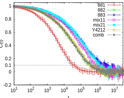
Relaxation timesIn this subsection we determine the longest relaxation time, τa, of the short arm. For this, we
analyze its end-to-end correlation function. This is defined as:
C(t) =hP(t)·P(t0)i
P2(t0)
0.1
-0.2 0 0.2 0.4 0.6 0.8 1
101 102 103 104 105 106 107
C(t)
t
[image:18.595.200.413.128.297.2]881 882 883 mix11 mix21 Y4212 comb
Figure 3: End-to-end correlators of the short arms for the different simulated systems. Symbols with error bars are simulation data. Solid lines are fits to a weighted sum of exponentials ( Eq. (18)). The dotted line indicates the upper level of noise.
where P(t),P(t0)is the end-to-end vector of the short arm at times t and t0respectively. When the
correlation function decays to 0 the short arm is fully relaxed. We show the correlation functions
of all the simulated systems in Figure 3. For each system we computed the end-to-end correlator
for 15 equispaced uncorrelated time origins t0. Each data set in Figure 3 is the average over the
corresponding 15 correlators. The error bars indicate, for each time t, the respective upper and
lower value obtained in the 15 correlators. In order to describe accurately the decay of the
end-to-end correlator and to get a reliable value ofτa, we fitted the simulation data of Figure 3 to
sev-eral empirical functions. The stretched exponential Kohlrausch-William-Watts (KWW) function,
gK(t)∝exp(−(t/τK)βK), whereβK <1 andτK are fit parameters, seems adequate for describing
the observed nonexponential decay of C(t). KWW fits provided a good description in most cases,
but failed for the 883-stars and for the two mixtures, which exhibit a more complex decay. An
alternative choice is to fit data to a weighted sum of exponential functions. Excellent fits (lines
in Figure 3) were obtained with five exponentials:
f(t) = 5
∑
i=1Even if the fitting function provides a very good description of our data, the strong noise in the final
decay of the correlation function makes the estimation ofτa rather tricky. However, it is evident
that the error bars in Figure 3 do not exceed the value C(t) =0.1. We define the longest relaxation
time of the short arm τa as the time at which the obtained fitting function drops to C(τa) =0.1.
This value of C(t)is rather small and at the same time, the noise at that level does not influence
significantly the estimated value ofτa. The average values ofτawith corresponding errors for the
simulated systems are listed in Table 2. In order to quantify the error of our estimation ofτa, we
fitted to Eq. (18) the 15 correlators computed for the different time origins. For each correlator we
obtained a relaxation time from the condition C(τa) =0.1, and we calculated the standard deviation
of the so-obtained 15 values ofτa.
0.5 1 1.5 2 2.5 3 3.5
102 103 104 105 106 107
<r
2 >/<ri 2 888
>
t 881
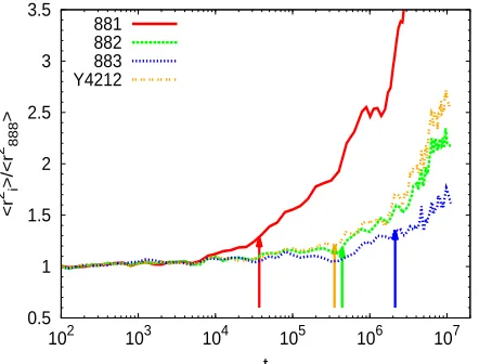
[image:19.595.192.413.367.535.2]882 883 Y4212
Figure 4: Ratio of the MSD of the T/Y-shaped asymmetric stars to the MSD of the reference symmetric stars as a function of time. The arrows are placed at the short arm relaxation timesτa
obtained by our method (see Table 2).
At this point it is worth studying the possible effect of the chosen method on the final value of
p2, namely by discussing other suggested approaches for obtaining τa from the simulation data.
There have been some attempts to determine the longest relaxation time of the short arm, τa,
from slip-link28and molecular dynamics simulations.18In the slip-link simulationsτawas defined
as the time when the short arm loses all its entanglements.28 In the MD simulations18 τa was
determined as the time at which the MSD of the branchpoint of the asymmetric stars deviates
that, after the short arm relaxation, the branchpoint is allowed to take a random hop along the
confining tube. This change in the branchpoint dynamics leads to a change in the slope of the
MSD. Zhou and Larson observed18 that this change occurred at the time when the end-to-end
correlation functions of the short arms decayed to C(t)≈0.2. However, there is no systematic
method to find an accurate time, where the MSD curves for asymmetric and symmetric stars split
up, so the values ofτa estimated by the naked eye have a significant uncertainty (up to one time
decade). Moreover, in order to obtain theτa for the mixtures we would need a reference system
consisting of a mixture of symmetric stars and linear chains. In Figure 4 we show the results
(arrows) obtained by our method (see above) together with MSD data of the branchpoint(hr2 ii)for
different architectures. The latter are divided by the branchpoint MSD of the reference symmetric
stars (hr2
888i). In this representation, deviations from the branchpoint motion of the reference
symmetric stars are reflected by deviations above the horizontal level hr2
ii/hr2888i=1. By direct
inspection of Figure 4 it seems that the precise point at which deviations arise is ill-defined (note
the scatter in the data). Still, it is clear that the so-defined relaxation times are systematically
smaller than those estimated by our method (arrows). As stated in Ref.,18 the time at which the
branchpoint MSD deviates from that of the reference symmetric stars is in very good agreement
with the time at which the short arm correlation function decays to C(t) =0.2. Obviously this
corresponds to a shorter time scale that the relaxation time used by us, obtained as C(τa) =0.1
(see above). Namely, the former is about a 50 % smaller than our corresponding value for τa,
which affects significantly the final value of p2.
In the case of the mixtures of asymmetric stars and linear chains, p2is obtained from Eq. (12),
which contains as additional parameter the relaxation time τs of the short linear chains in the
mixture. We proceeded in a similar manner as for the short arms in the branched polymers, by
analyzing the end-to-end correlator of the linear chains. However, the relaxation time of the linear
chains is obtained in the usual way, as C(τs) =e−1, unlike the condition C(τa) =0.1 used for the
4.3
Tube diameter and tube survival probabilityAs mentioned in the Introduction, one of the open questions regarding branchpoint dynamics is
whether hopping takes place in the skinny (undilated) or in the fat (dilated) tube. In this subsection
we investigate both cases and estimate from the simulation the corresponding values for the tube
diameter. First we calculate the original skinny tube diameter, a0, in our bead-spring polymers as:
a20=NePPC∞b20, (19)
where C∞ is the characteristic ratio, b0 is the average bond length, and NePP is the entanglement
length estimated by primitive path analysis. We find b0= 0.97, and by analyzing the
asymp-totic behavior of intramolecular distances between distant beads (see Ref.37for details), we obtain
C∞b20=3.46±0.10 for all systems. We use the value NePP =23 reported by Everaers et al.,35
which was obtained for a melt of bead-spring chains at the same density and temperature, and with
identical interactions as those used in our work. By inserting the former values in Eq. (19), we
obtain a diameter a0=8.92±0.13 for the skinny tube.
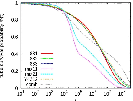
In order to quantify the diameter of the fat tube for each investigated system, we first need
to analyze the corresponding tube survival probabilityΦ(t).38 The procedure for obtaining Φ(t)
involves the calculation of the tangent correlation functions of polymer segments for the different
investigated architectures. These provide information on the relaxation times of the primitive path
coordinates, which can be used to determine the time dependence of the tube survival probability.
A detailed description of the procedure is given in the Appendix. The obtained results for the tube
survival probabilities are represented in Figure 5. The dilated tube diameter at the relaxation time
τaof the short arm can be obtained as:6,8
a2= a 2 0
Φα(τa) (20)
α is the dilution exponent. In the analysis of the hopping parameter p2(see below) we will
con-sider the two suggested values of the dilution exponent,8 α =1 and α =4/3. As we discussed
in the previous subsection, for each simulated system we use a set of 15 end-to-end correlators
(computed at distinct time origins), yielding their respective values ofτa. Accordingly, we have a
corresponding set of 15 values forΦ(τa). We use these for computing the standard deviations of
Φ(τa)(see below).
The calculated tube survival probability is directly related to the parameter φα in Eq.
(11)-Eq. (12) via:
φα =Φα(τ
a). (21)
This parameter represents the fraction of the material that is responsible for the slow constraints in
the system. After the relaxation of the fastest parts in our systems (short arms, and linear chains
in the mixtures), the only slow components to relax are the long arms or main backbone. This
information is contained in Φ(τa), which measures the unrelaxed tube fraction at τa, i.e., at the
time scale of the relaxation of the short arm. This is also the case for the investigated star/linear
mixtures. Indeed the relaxation time for the linear chains is, at most, that of the short arms, since
both have the same length (three entanglements, see Figure 1), but the short arms have only one
free end.
0 0.2 0.4 0.6 0.8 1
101 102 103 104 105 106 107 108
tube survival probability
Φ
(t)
t 881
[image:22.595.193.413.545.713.2]882 883 mix11 mix21 Y4212 comb
0 0.2 0.4 0.6 0.8 1
101 102 103 104 105 106 107 108
tube survival probability
Φ
(t)
t Asymmetric star 882
Simulation data BoB p2=1.0 α=4/3 BoB p2=1/60 α=1.0
0 0.2 0.4 0.6 0.8 1
101 102 103 104 105 106 107 108
tube survival probability
Φ
(t)
t
Mix asymmetric star(883):linear chain 1:1
[image:23.595.192.414.121.480.2]Simulation data BoB p2=1.0 α=4/3 BoB p2=1/60 α=1.0
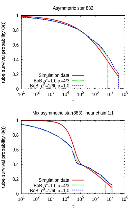
Figure 6: Comparison between the tube survival probabilities obtained from the simulations (solid line) and from the BoB model with choice of parameters p2=1,α =4/3 (dashed line) and p2=
1/60,α =1 (dash-dot line).
Some general trends are inferred from simulation data in Figure 5. The two mixtures exhibit
an abrupt decay in the range 104.t .105. The beginning of this decay is consistent with the
estimated relaxation time of the linear chains (τs =19000, see above). Thus, completion of the
relaxation of the short linear chains leads to a sharp removal of constraints. As expected, the
larger fraction of linear chains in the mixture 1:1 produces a stronger decay of Φ(t) than in the
mixture 2:1. Differences in the tube survival probabilities of the T-shaped stars (881, 882, and
883) and the Y4212-stars are small at all time scales, which suggests a relatively small role of
the relaxation of the short arms in the total Φ(t) of these systems, and once the short arms are
of combs is markedly different from that of the T- and Y-stars. It shows a faster decay up to time
scales of aboutτa. This is consistent with a stronger role of dynamic tube dilution in combs, due
to their higher volume fraction of short arms than in the T- and Y-stars. However, after relaxation
of the short arms, the combs contain two frictional fat beads close to the both ends of the linear
backbone. This strongly hinders relaxation andΦ(t)exhibits a very slow decay over the following
time decades, prior to the late decay by reptation.
The tube survival probabilities obtained from the simulations can be directly compared with
theoretical predictions from hierarchical models. Here we compare our results with those from
the branch-on-branch (BoB) model developed by Das et al. (see Ref.3 for details). The BoB
model makes detailed predictions for linear rheological data of non-looped branched architectures
of arbitrary complexity, by using the entanglement length and entanglement time as external inputs.
Output of the BoB calculation includes the tube survival probabilityΦ(t). Figure 6 compares BoB
and simulation results ofΦ(t)for some representative cases (882-stars and star/linear mixture 1:1).
BoB assumes a priori values forα and p2. The results in Figure 6 are obtained for two limit cases
p2 =1/60, α =1 (dash-dot lines), and p2=1, α =4/3 (dashed lines). These include the two
values used for the scaling exponent α and the lowest and highest value of p2 reported in the
literature.11Both the hopping parameter p2and the scaling exponent (through the factorΦ−α(τa))
determine the friction constant for the final reptation of the system. Therefore, in systems where
final relaxation is mediated by reptation, decreasing the values of p2 and α moves the reptative
regime to longer timescales. Thus, the cases p2=1/60, α =1 and p2=1, α =4/3 provide an
upper and lower bound for the onset of reptation predicted by BoB. Relaxation by reptation in the
BoB curves of Figure 6 corresponds to the final sharp drop to zero.3This time scale can change by
even one decade according to the specific choice of p2 andα.
Having noted this, the chosen values of p2 andα do not significantly affect the obtained BoB
curves in the time window, t≤τa(relaxation before arm retraction is independent of p2and
chang-ingα from 1 to 4/3 introduces less than 0.1% difference inΦ(t) atτa for the molecules
information onΦ(t)at the relaxation time of the short armsτa(through equations for the
diffusiv-ity in Section 3 and Eq. (21)), i.e., much before the onset of reptation. As shown in Figure 6 the
two limit cases of p2andα used to generate the BoB curves lead to essentially the same results in
the former time window, differences only arising at much longer times. Still, it must be noted that
α should have a significant effect in that window for long side arms. In the cases investigated here
the effect is negligible because the side arms are weakly entangled and stay in the early fluctuation
regime.
In general, the simulation results for the tube survival probability are in qualitative agreement
with the corresponding BoB results. The agreement is even semiquantitative in the case of the
pure T-stars. The BoB model captures the trends observed by simulations, including the crossover
between fast dynamics of the short linear chains/side branches and slow relaxation of the long
backbone. Having said this, it must be noted that for some systems (Y4212-stars and combs)
a significant part of the final relaxation of the backbone occurs at times beyond the simulation
window (t&4×10⁷), so conclusions about the comparison at such time scales must be taken with
care.
Once the reptation plateau in hr2i/t1/2, as well asτ
a and Φ(τa)have been determined from
the simulations, we can directly obtain the actual value of p2 (see Section 6). According to the
discussion in Section 3, different expressions will be used for p2. These will depend on the specific
architectures and compositions (pure or mixture), as well as on the choice of hopping in the dilated
or in the skinny tube. In the different expressions of p2, the values of τa and Φ(τa) will enter
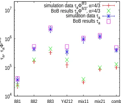
separately and/or through the productτaΦ2α(τa)(see Section 6). Figure 7 shows simulation results
ofτa and the productτaΦ2α(τa), for the case of dilution exponentα =4/3, in comparison with
the corresponding results obtained from the BoB model. A good agreement is again found, with
some tendency for overestimation by BoB. Similar agreement is observed for the caseα =1. With
all this, we conclude that our procedure provides a robust estimation of tube survival probabilities
and relaxation times of the short arms, allowing for a reliable estimation of the hopping parameter
104 105 106 107
881 882 883 Y4212 mix11 mix21 comb
τa
,
τa
Φ
8/3
[image:26.595.208.403.130.296.2]simulation data τaΦ8/3, α=4/3 BoB results τaΦ8/3, α=4/3 simulation data τa BoB results τa
Figure 7: Comparison of the simulation results ofτaandτaΦ2α(τa)with BoB predictions for the
dilution exponentα =4/3.
4.4
Branchpoint trajectoriesA further test of consistency for the estimated arm relaxation times can be obtained by analyzing
the real-space trajectories of the branchpoints. Hierarchical models postulate branchpoint diffusion
after relaxation of the short side arms. Prior to this, the branchpoint remains strongly localized. In
order to test this hypothesis we have analyzed the shape of the trajectories at different time scales.
Thus, for times t >105 we have saved the coordinates of the branchpoint every τ =2000 time
units. This roughly corresponds to one entanglement time (τe=1800). At earlier times we have
used shorter intervals for saving the branchpoint positions. Namely we have used τ =2×10n−2
for the time decade 10n<t ≤10n+1, with 2≤n≤4. With this, we use a large number of points
(at least 50) to characterize the shape of the branchpoint trajectory at any relevant time. This
characterization can be made by computing the asphericity parameter, defined as:
A= (I2−I1) 2+ (I
3−I1)2+ (I3−I2)2
2(I1+I2+I3)2
(22)
where I1,I2,I3are the semiaxes of the inertia ellipsoid of the trajectory. Thus, at each selected time
t, we compute the asphericity A(t)of the set of points consisting of the saved branchpoint positions
withτ the interval for saving used in the time decade which t belongs to (see above). For example,
for t=4×10³, we use the branchpoint positions at t′≤t saved every 20 time units. For any time
t>105 we use those saved every 2000 time units. In this way we get a fair characterization of
the asphericity at any time, by always analyzing a set of points equispaced in time, and preventing
‘crowding’ in the regions visited by the branchpoint during the early time decades.
0.15
0.01 0.1
102 103 104 105 106 107
Asphericity
A
t
random walk
[image:27.595.194.414.250.421.2]888 881 882 883 mix11 mix21 Y4212 comb
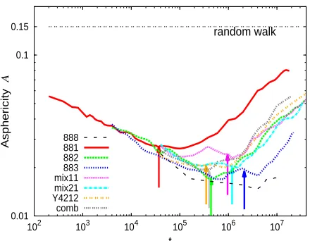
Figure 8: Time dependence of the asphericity of the branchpoint trajectory for all the simulated systems. The horizontal line represents the limit case of a random walk. The arrows indicate the relaxation timesτa of the short arms, as determined independently from the analysis of their
end-to-end correlators (see text).
Figure 8 shows the time dependence of the asphericity of the branchpoint trajectory for all
the investigated systems. For comparison we include the value A≈0.15 obtained for a particle
performing a three-dimensional random walk. The evolution of the asphericity with time reveals
interesting features. In the early stage of the simulation, the asphericity diminishes by increasing
time. This means that new positions of the branchpoint become localized in a limited region of
the space, forming a trajectory that becomes closer and closer to the ideal spherical shape (A=0).
The asphericity reaches a minimum and then increases with time during the rest of the simulation,
i.e., the branchpoint trajectory becomes progressively unlocalized. The random-walk limit is not
reached at the end of the simulation. This will happen at much longer time scales, in the
three-dimensional isotropic diffusive regime,hr2(t)i∝t. Note that for the asymmetric systems, only
window.
The minimum in the asphericity seems to follow several trends. For the three investigated
T-shaped stars, it becomes deeper, i.e., the branchpoint becomes more localized, by increasing the
length of the short arm. As expected, the strongest localization is found for the symmetric
888-stars. Localization in the 883-stars becomes weaker by mixing with short linear chains. In Figure 8
we have indicated (arrows) the relaxation timesτaof the short arms, as obtained by the method
pre-sented in Section 4B. Within statistical error, there is a clear correlation between these time scales
and the end of the localization of the branchpoint and later increase of the asphericity from the
minimum. This result is consistent with the theoretical assumption of hopping of the branchpoint
after full relaxation of the short arm.
5
Analysis: experimentsWe use results from linear rheology measurements on a series of polystyrene (PS) and polyisoprene
(PI) combs.17,42 The mastercurves obtained from the dynamic frequency sweep measurements
correspond to reference temperatures Tref=0◦C for polyisoprene and Tref=170◦C for polystyrene.
Similarly to the simulation analysis, estimation of the arm relaxation time from comb experimental
data presents some difficulties. In an effort to identify the arm relaxation time of the combs and to
check the consistency of the obtained values we have used three different methods:
1. Analysis of the tube survival probabilities provided by the BoB computational algorithm. In
this calculations we explicitly use the experimentally determined polydispersity indices in
arm lengths (less than 1.1 in all cases).
2. Analysis of the intermediate peak in the frequency dependence of the experimental loss
tangent tanδ =G′′(ω)/G′(ω).
3. Defining the time at which G(t) =Geφunr2 , where G(t)and Ge are the experimental stress
relaxation function and entanglement modulus, respectively. The quantityφunris the fraction
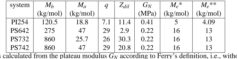
Table 1: Molecular characteristics17,42,45 and parameters used in the estimation ofτaof the
exper-imental combs.
system Mb Ma q Zdil GN Me* Me**
(kg/mol) (kg/mol) (MPa) (kg/mol) (kg/mol)
PI254 120.5 18.8 7.1 11.4 0.41 5 4.09
PS642 275 47 29 2.9 0.22 16 13
PS732 860 25.7 26 30.3 0.22 16 13
PS742 860 47 29 20.8 0.22 16 13
*Mewas calculated from the plateau modulus GN according to Ferry’s definition, i.e., without the
4/5 prefactor.43
**Mewas calculated from the plateau modulus GN according to the definition used in BoB and
Fetters et al.,44i.e., with the 4/5 prefactor.
102 103 104 105 106 107
10-4 10-3 10-2 10-1 100 101 102 103 104 105 106
G
’,
G
’’ (Pa)
frequency ω (rad/s)
G’ BoB prediction
G’’ BoB prediction
G’ data PI254
G’’ data PI254
[image:29.595.198.417.483.670.2]The molecular characteristics of the combs are described in Table 1. All combs have a long
well-entangled backbone (Zb in the approximate range of 17 to 54 entanglements). The arms are
weakly or moderately entangled (Za in the range of 1.6 to 6 entanglements). The values of Zdil
in Table 1 have been calculated by using Eq. (13) and entanglement molar masses Me obtained
from the Ferry’s definition (column 7 in Table 1). The terminal relaxation times of the arms and
backbone (see Table 5) differ by several orders of magnitude and therefore, it becomes possible
to separate the two relaxation processes by using only linear rheology. The first method used to
identify relaxation times includes the use of the BoB computational algorithm.3 Figure 9
com-pares experimental data and BoB results for the PI254 comb at reference temperature Tref=0◦C.
The input parameters required by BoB are the entanglement molecular weight Me, entanglement
time τe, dilution exponent α and hopping parameter p2. We set α =1 for all the studied
sys-tems. Good agreement with the experimental moduli is achieved by using Me(PI) =4.09 kg/mol
and τe(PI) =10−4 s at Tref =0◦C. In the case of the PS combs we use Me(PS) = 13 kg/mol
and τe(PS) =5×10⁻⁴ s at Tref =170◦C. The entanglement times τe chosen are shown to be
consistent with previous works for the PS combs17 and for the PI comb.19,46 The plateau moduli
corresponding to this set of parameters (listed in Table 1) are in agreement with published results
of experimentally estimated GN.47 Whereas the PI microstructure is ≥90% 1,4-addition, even a
small variation may slightly change the entanglement modulus Ge andτe. This may explain small
variations in the values of these parameters in this and other works, but overall there is consistency.
Architectural variability such as polydispersity in arms and backbone or uncertainty in the
num-ber and position of the branches is another possible source of discrepancy.17 Although the TGIC
(temperature gradient interaction chromatography) characterization on the PS combs confirmed
their high level of purity (>85% target material),42,48 the samples are still not perfect in terms of
microstructural architecture. However, given the anticipated small effect,24 further fractionation
was not performed and this has not been further pursued in this work.
It must be noticed, that the molecular entanglement length defined in BoB is by a factor 4/5
the different definitions of Me (see43 for more details). The value of p2 was selected to describe
well the low frequency region of G′ and G′′ 1. It is important to stress, as we discussed in
Sec-tion 4.3, that the value of p2 chosen for BoB prediction is irrelevant for further estimation ofτa.
Once we checked that BoB provides a good description of the linear rheological data we used
ad-ditional output from BoB to estimate the arm relaxation time. Namely, by using the tube survival
probability computed by BoB,3Φ(t), we obtain the arm relaxation timeτa as the time for which
Φ(τa) =φunr, withφunr given by Eq. (23) below. Similarly to the work of Kapnistos et al.,17 we
include the contribution of the free backbone ends, and calculate the fraction of unrelaxed material
after the full arm retraction as:
φunr=1−(φa+φe) =1−
qMa+2Mb/(q+1) qMa+Mb
, (23)
whereφaandφeare the volume fraction of the arms and dangling backbone ends, respectively. The
factor q is the number of side arms per comb. The quantities Mband Maare the molecular masses
of the backbone and of each of the side arms, respectively. The values of all quantities included
in Eq. (23) are given in Table 1.
0 0.2 0.4 0.6 0.8 1
10-5 10-4 10-3 10-2 10-1 100 101 102 103 104 0.1 1 10 100
Φ
(t)
tan
δ
time (s)
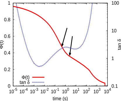
[image:31.595.197.404.506.679.2]Φ(t) tan δ
Figure 10: Unrelaxed volume fractionΦ(t)obtained from BoB (solid line) and experimental tanδ (dashed line) versus time, for the PI254 comb. The arrows indicate the values ofτa′ andτaobtained
by usingΦ(τa′) =1−φaandΦ(τa) =1−(φa+φe), respectively.
We have also determined the time τa′ at which the fraction of unrelaxed material is given by
Φ(τa′) =1−φa. This gives us a lower bound for the estimation of the arm relaxation time.
Fig-ure 10 shows the time dependence of the functionΦ(t)obtained by the BoB model for the case of
PI254. We indicate (arrows) the timesτa′ andτa, obtained from the BoB model as explained above.
For comparison, we plot in the same figure the experimental loss tangent versus inverse frequency.
The intermediate peak in tanδ falls in between the two relaxation timesτa′ andτa. From the plot of
unrelaxed fraction versus time we can identify two main relaxation processes. The final relaxation
time of the arms is at the transition point between these two processes. We find the same
qualita-tive behavior than in theΦ(t)of the simulated combs ( Figure 5), with a very slow decay afterτa
extending over several decades prior to the final reptational decay.
In the second method we determine τa by analyzing the intermediate peak in the frequency
representation of the experimental tanδ. The first step is to fit the curves with, e.g., a Gaussian or a
Lorentzian function. One example of the fitting procedure is shown in Figure 11. Then we estimate
τaas the inverse of the peak of the so-obtained fitting function. Another estimation can be obtained
from the derivative of the experimental tanδ-curve, by definingτaas the inverse frequency at the
[image:32.595.188.425.509.686.2]point in which the derivative becomes zero.
Figure 11: Symbols: frequency dependence of tanδ for the PS642 comb (log-log representation). The line is a Gaussian fit of the peak. αT is the horizontal shift factor, for the presented data
Finally, we make another estimation of the arm relaxation time by analyzing the experimental
stress relaxation modulus G(t). The tube model in combination with the dynamic dilution
the-ory41 provides an expression for the relaxation modulus G(t)consisting of two contributions: (i)
fast Rouse modes together with longitudinal Rouse modes in the tube that represent 1/5 of the Ge
relaxation, (ii) escape from the tube at longer times related to the plateau modulus GN =45Ge. One
may generally assume that, at the times comparable to the relaxation time of the side arms, the first
contribution has already relaxed. However, in the comb architecture where the longitudinal modes
are primarily operative at the backbone, this relaxation mechanism may depend on the number and
position of branchpoints on the backbone. In all experimental combs used for this analysis the
average distances between the branchpoints are very small, in most cases Zdil/q≪1. Therefore
the relaxation modes involving the motion of the backbone along the tube are frozen during the
relaxation of the side arms. Only small fluctuations of the backbone between consecutive
branch-points are present. Following this argument and assuming a dilution exponent α =1,17,19,24 at
the end of the arm relaxation the relaxation modulus will be G(τa) =Geφunr2 instead of the value
G(τa) =GNφunr2 expected for Zdil/q>1. We would like to draw attention to this issue, because
the suppression of the longitudinal Rouse motion seems to be a general feature of densely grafted
combs. We use in the calculation an entanglement modulus Ge= 54GN =5.1×10⁵ Pa for PI and
Ge=2.8×10⁵Pa for PS. These values are consistent with the above reported values of Me, in the
sense that they obey rubber elasticity49 within 15% at reference temperatures given above.
Fig-ure 12 shows experimental results for the relaxation modulus in the different investigated systems.
We indicate by arrows the corresponding values ofτaestimated by this method.
By combining the results obtained by the different methods presented in this section, we
de-termine an upper and lower bound for the arm relaxation timeτain each of the investigated comb