This is a repository copy of
Obstructions for linear rank-width at most 1
.
White Rose Research Online URL for this paper:
http://eprints.whiterose.ac.uk/101103/
Version: Accepted Version
Article:
Adler, I, Farley, AM and Proskurowski, A (2014) Obstructions for linear rank-width at most
1. Discrete Applied Mathematics, 168. pp. 3-13. ISSN 0166-218X
https://doi.org/10.1016/j.dam.2013.05.001
© 2013, Elsevier. Licensed under the Creative Commons
Attribution-NonCommercial-NoDerivatives 4.0 International
http://creativecommons.org/licenses/by-nc-nd/4.0/
eprints@whiterose.ac.uk https://eprints.whiterose.ac.uk/ Reuse
Unless indicated otherwise, fulltext items are protected by copyright with all rights reserved. The copyright exception in section 29 of the Copyright, Designs and Patents Act 1988 allows the making of a single copy solely for the purpose of non-commercial research or private study within the limits of fair dealing. The publisher or other rights-holder may allow further reproduction and re-use of this version - refer to the White Rose Research Online record for this item. Where records identify the publisher as the copyright holder, users can verify any specific terms of use on the publisher’s website.
Takedown
If you consider content in White Rose Research Online to be in breach of UK law, please notify us by
Obstructions for linear rank-width at most 1
Isolde Adler1⋆, Arthur Farley2, and Andrzej Proskurowski2
1
Institut fur Informatik, Goethe-Universitat, 60325 Frankfurt, Germany iadler@informatik.uni-frankfurt.de
2
University of Oregon, Eugene, OR 97403-1202, USA andrzej,art@cs.uoregon.edu
Abstract We establish the set of minimal forbidden induced subgraphs for the class of graphs having linear rank-width at most 1. From these we derive both the vertex-minor and pivot-minor obstructions for the class.
1 Introduction
Rank-width is a graph parameter introduced by Oum and Seymour [16] as an efficient approximation of the clique-width [6] of a graph. Linear width is obtained from width by restricting the trees in the decomposition to caterpillars. Intuitively, linear rank-width is related to rank-rank-width in the same way as path-rank-width is related to tree-rank-width. Large classes of graph problems that are NP-hard in general become tractable when restricted to graphs of bounded (linear) rank-width [5,8,10,13]. While the structure of graphs of bounded path-width is well understood [3,7,12,17], much less is known about graphs of bounded linear rank-width. Indeed, linear rank-width generalizes path-width in the sense that if a graphGhas path-width at mostkthenGhas linear rank-width at mostk(this is not hard to prove, cf. [1]). Recently, Ganian [9] introduced the class of thread graphs and proved that the graphs of linear rank-width at most 1 are precisely the thread graphs.
In this paper, we characterize the graphs of linear rank-width at most 1 in three ways: firstly by induced subgraph obstructions, secondly by vertex-minor obstructions and thirdly by pivot-minor obstructions. More precisely, let≤be a quasi-ordering (i.e. a reflexive and transitive ordering) on graphs, and let C be a class of graphs that is downward-closed under ≤. A graph G is an obstruction for C if G /∈ C and H ∈ C for every H G. For example, Kuratowski’s famous theorem states that the obstructions for planar graphs w.r.t. (topological) minor containment are the two graphsK5 and K3,3.
For the class of graphs of linear rank-width at most 1, we determine the set of obstruc-tions w.r.t. induced subgraph containment (cf. Theorem 4 and Figure 3), w.r.t. vertex-minor containment (cf. Theorem 25 and Figure 5), and w.r.t. pivot-minor containment (cf. The-orem 26 and Figure 9). It is known that the obstruction sets for graphs of bounded linear rank-width w.r.t. vertex-minor and pivot-minor containment are finite [14,15]. However,
until now none of these obstruction sets were known explicitly. Obstruction set character-izations are known for the class of graphs of rank-width at most 1 (i.e. for the distance hereditary graphs) [2] and for the class of circle graphs [4]. To obtain our results, we de-pend upon the known equivalence between graphs of linear rank-width at most 1 and thread graphs [9] and the fact that we can reduce the search for unknown obstructions to distance-hereditary graphs.
In Section 2, we introduce basic notions and known facts. In Sections 3 and 4 we find the induced subgraph obstructions, from which we obtain the vertex-minor obstructions in Section 5 and the pivot-minor obstructions in Section 6.
2 Definitions
We consider finite, simple graphs, each graphGconsisting of the set V(G) of vertices and the set E(G) of edges, every edge e ∈ E(G) being a two-element subset of V(G). Given an edge e={u, v}, we say that u isadjacent to v and eis incident with bothu and v. A sequence v0, v1, ..., vk of vertices ofG, no two being equal and every consecutive pair being
adjacent is called apath. The length of a path isk, the number of its edges. If additionally v0 andvk are adjacent, they form a cycle. A graph without a cycle is calledacyclic. For a
vertex v, we letNG(v) :=
u∈V(G)
{u, v} ∈E(G) be theneighborhood of vinG. The degree of v ∈V(G) is degG(v) := |NG(v)|. A vertex of degree 1 is a pendant vertex, and
the edge incident with a pendant vertex is a pendant edge. A graph H is a subgraph of G ifV(H)⊆V(G) and E(H)⊆E(G). For a subsetX ⊆V(G), letG[X] be the subgraph of G induced by X, i.e.V G[X]
=X and E G[X]
:= {e∈ E(G) |e⊆ X}. Such a graph H is an induced subgraph of G. For a subset Y ⊆V(G), we let G\Y :=G[V(G)\Y]. If Y ={y} is a singleton set, then we writeG\y instead ofG\ {y}.
A graph G is connected if G6=∅ and any two vertices ofG are connected by a path. A graph G that is not connected is said to be disconnected. Aconnected component of G is a maximal connected subgraph of G. We say that a vertexv ∈V(G) is a cut-vertex if G\v has more connected components thanG. Atree T is an acyclic connected graph. We denote the set of leaves of T by L(T). Any vertex in V(T)\L(T) is aninternal vertex. A tree is cubic if it has at least two vertices and every internal vertex has degree 3. For an integer n≥3, we let Cn denote the n-cycle, i.e. the cycle with n vertices. For a graph G
containing a cycle, a chord in the cycle is an edge of G between two vertices of the cycle that are not consecutive. Acomplete bipartite graph is a graphGwith a bipartition [X, Y] of V(G) such thatE(G) =
{x, y} |x∈X and y∈Y .
⊕p: Add a new pendant vertexvconnected by an edge to an existing vertexuof the graph. ⊕f: Add a new vertex v with the same set of neighbors as a vertex u of the graph. The
verticesu and v are called false twins of each other.
⊕t: Add a new vertexvwith the same set of neighbors as a vertexuof the graph, connecting
u and v by an edge. The verticesu and v are calledtrue twins of each other.
We denote a dh-operation acting on a vertexuof a graphGby⊕x(G, u), wherex∈ {p, t, f}.
LetM(G) denote the adjacency matrix of a graphG,i,e.,M(G) is the|V(G)| × |V(G)| matrix where the columns and the rows are indexed by the vertices of G, and M(G) has entries in {0,1}, where the entry mi,j = 1 if and only if the corresponding row vertex
is incident to the corresponding column vertex. For a bipartition [X, Y] of V(G), we let M(G)[X, Y] denote the|X|×|Y|submatrix (mi,j)i∈X,j∈Y ofM(G). Thecutrank function of
a graph Gis defined by cutrkG: 2V(G)→Ngiven by cutrkG(X) := rank M(G)[X, V(G)\
X]
, where rank is the rank function over GF(2). A rank-decomposition of a graph G is a pair (T, λ), whereT is a cubic tree and λ:L(T) → V(G) is a bijection. For every edge e∈E(T), the two connected components ofT\einduce a partition (Xe, Ye) ofL(T). The
width of e is defined as cutrkG(λ(Xe)). The width of a rank-decomposition (T, λ) is the
maximum width over all edges of T. Therank-width of Gis defined as
rw(G) := min{width of (T, λ)|(T, λ) rank-decomposition ofG}.
If |V(G)| ≤1, then Ghas no rank-decomposition and we let rw(G) = 0.
Proposition 1 ([14]) A graphG is distance-hereditary if and only if rw(G)≤1.
Linear rank-width is a related concept that restricts the form of the rank-decomposition. A caterpillar is a treeT in which the removal of all leaves results in a path. Alinear rank-decomposition of a graph G is a rank-decomposition (T, λ) of G, where T is a caterpillar. The linear rank-width ofG is defined as
lrw(G) := min{width of (T, λ)|(T, λ) linear rank-decomposition ofG}.
Equivalently, lrw(G)≤kif there exists a permutationπ ofV(G) such that for every prefix X ofπ cutrkG(X)≤k. If|V(G)| ≤1, thenGhas no linear rank-decomposition and we let
lrw(G) = 0.
Obviously, lrw(G) ≥ rw(G), and lrw(G) ≤ k implies rw(G) ≤ k. It is easy to verify that cliques, caterpillars and complete bipartite graphs have linear rank-width at most 1 and that the disjoint union of two graphs G and H has linear rank-width equal to max{lrw(G),lrw(H)}.
Example 2 The cycle C5 satisfieslrw(C5) = 2. In any linear rank-decomposition(T, λ)of
C5 every edge in E(T) between two internal vertices of T has width2, and every pendant
3 Induced subgraph obstructions
The class of graphs with linear rank-width at most k is closed under induced subgraphs, i.e.,if a graphGsatisfies lrw(G)≤kthen lrw(H)≤kfor all induced subgraphsHofG. We define the set of induced subgraph obstructions (or minimal forbidden induced subgraphs) for the class of graphs G such that lrw(G) ≤1, denoted as O, as all graphs G such that lrw(G) > 1 and lrw(G\v) = 1 for all vertices v in G. Such obstructions are necessarily connected.
Lemma 3 Every graphG∈ O is connected.
Proof. Assume a graph G ∈ O is not connected. Then we can delete a vertex v in one of
the connected componentsC of Gand find that the resulting graph has linear rank-width at most 1. Each of the unaffected components must have linear rank-width≤1. Similarly, by deleting a vertex v′ in a different component C′ 6= C of G, we find that lrw(C) ≤ 1. SinceGis the disjoint union of its components, it follows that lrw(G) = 1, a contradiction.
We will prove the following theorem.
Theorem 4 The set of induced subgraph obstructions for graphs having linear rank-width at most 1 consists of the induced subgraph obstructions for distance-hereditary graphs and the graphs shown in Figure 3.
It follows from Proposition 1 that the class of graphs having linear rank-width at most 1 is a subclass of distance-hereditary graphs. Hence, to prove Theorem 4 it suffices to show thatO consists of the induced subgraph obstructions for distance-hereditary graphs and the obstructions that are themselves distance-hereditary graphs, which are the graphs shown in Figure 3.
The set of induced subgraph obstructions for distance-hereditary graphs, denoted as D, has been shown to consist of exactly the following elements: [2]:
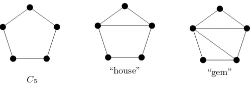
•any cycle of length five or greater (“holes” of length at least 5), •a 5-cycle with one chord (“house”),
•a 5-cycle with two non-crossing chords (“gem”), and
•a 6-cycle with a chord connecting two vertices at distance 3 along the cycle (“domino”).
Lemma 5 Dis a subset of O.
Proof.By inspection, for every graphGinD, lrw(G) = 2 and lrw(G\v) = 1, for all vertices
v in G. Therefore, these graphs are also induced subgraph obstructions for graphs having
To complete the specification of the setOit is necessary to determine the set of distance-hereditary graphs that are induced subgraph obstructions for graphs with linear rank-width at most 1. We denote this set of obstructions asOdh.
Lemma 6 O =D ∪ Odh.
Proof.By Lemma 5, it suffices to show thatO \ D ⊆ Odh. LetG∈ O \ D. Then lrw(G)≥1,
rw(G) ≤ 1 by Proposition 1, and, for all v ∈ V(G), 1 = lrw(G\v) = rw(G\v). Hence
G∈ Odh by definition.
To determine the setOdh, we consider an alternative characterization of graphsGwith
lrw(G)≤1 introduced in [9] calledthread graphs. Here, we define thread graphs and note some of their relevant properties. It can be easily seen that our definition is equivalent to the original definition in [9].
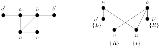
A thread block is the basic building block of a thread graph. A thread block B is a tuple (G,(a, b),v,¯ L), consisting of a graph G, a distinguished edge {a, b} ∈E(G), called thethread edge of G, an ordering ¯v= (v1, . . . , vn) of the vertices of V(G)\ {a, b}, called a
thread ordering, and an associated thread labeling L:V(G)\ {a, b} → {L, R,∗}, such that
• for all 1≤i < j≤n,{vi, vj} ∈E(G) if and only ifL(vi)∈ {R,∗} and L(vj)∈ {L,∗}. • for all 1≤j≤n,{a, vj} ∈E(G) if and only ifL(vj)∈ {L,∗}.
• for all 1≤j≤n,{vj, b} ∈E(G) if and only if L(vj)∈ {R,∗}.
Intuitively, in the sequence (a, v1, . . . , vn, b) every vertexuwithL(u)∈ {L,∗} ‘sees’ all
vertices v to its left that ‘look’ to the right, i.e.,that have L(v) ∈ {R,∗}. Symmetrically, every vertexvwithL(v)∈ {R,∗}‘sees’ all verticesuto its right that ‘look’ to the left,i.e., that have L(u)∈ {L,∗}. The label “∗” can be understood to represent both labels, i.e.,to be the set{L, R}.Verticesaandbare calledthread verticesand are implicitly labeled “∗”. A thread block istrivialif it consists of only the thread edge. A non-trivial thread block may have a cut-vertex, as it may include pendant vertices. Figure 1 shows graph G with an edge {a, b}, an ordering ¯v = (a′
, v, u, b′
) and a labelingL such that (G,(a, b),¯v,L) is a thread block.
a′ a
b b′
u v
a′
{L}
a b
b′
{R}
u v
[image:6.612.154.420.530.614.2]{R} {∗}
Aconnected thread graph Gis either a single vertex or a sequence of thread blocks Bi,
1 ≤ i ≤ n, such that thread vertex bi of thread block Bi is identical with thread vertex
ai+1 of thread blockBi+1, for 1≤i≤n−1. We call this shared vertex a bridging vertex.
A consistent threading of a connected thread graph G is an assignment of a sequence of edges that form a path to be thread edges, and an ordering and labeling of non-thread vertices, such that the edges implied by the ordering and labeling correspond to the edges ofG. From now on we only consider consistent threadings of thread graphs where the first and the last thread block are non-trivial. This is not a restriction, because a trivial thread block is a pendant edge and may be folded into the neighboring thread block.
A thread graph G is either the empty graph or a disjoint union of connected thread graphs. Aconsistent threading of a thread graph is a collection of consistent threadings of its connected components.
The following property of thread graphs follows immediately from the definitions.
Remark 7 Let G be a thread graph. The set of bridging vertices is the same for every consistent threading of G, and every bridging vertex is shared by exactly two thread blocks. ⊓ ⊔
The structure of a thread block can be represented concisely by the sequence (l1, . . . , ln)
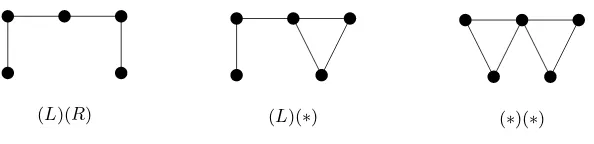
of vertex labels of the non-thread vertices (e.g.,(L, R,∗, R) for the graph in Figure 1). A sequence of thread blocks can likewise be represented as a sequence of non-thread vertex label sequences of the thread blocks (e.g., (L, R)(∗) for a two block sequence). Minimal thread blocks involve single non-thread vertices.
Remark 8 Every connected thread graph of three or more vertices has one of the following thread blocks as an induced subgraph: (R),(L), or (∗).
From these graphs the set of non-isomorphic, minimal two-block thread graphs can be determined and are useful for determining certain obstructions.
Lemma 9 The vertex-minimal thread graphs with two non-trivial thread blocks are(L)(R), (L)(∗), and (∗)(∗), which are unique up to an isomorphism.
Proof.The thread graphs (R)(R),(R)(∗),(R)(L) can be represented as the one-block thread
graphs (LLR),(LL∗), and (LLL), respectively. (L)(L) and (∗)(L) are isomorphic to the first two of these graphs, respectively. Also, (∗)(R) is isomorphic to (L)(∗), so we have accounted for all 9 vertex-minimal non-empty thread graphs with two thread blocks.
(L)(R) (L)(∗) (∗)(∗)
Figure 2.The three graphs of Lemma 9.
The following theorem showing equivalence between the class of thread graphs and graphsGwith lrw(G)≤1 was proven in [9]. We give a related proof here for completeness.
Theorem 10 (Ganian [9]) A graph Ghaslrw(G)≤1if and only if Gis a thread graph.
Proof. We may assume thatGis connected and E(G)6=∅.
(⇒) Assume lrw(G) ≤ 1, and let (T, λ) be a linear rank-decomposition witnessing this. Consider a total ordering≺of the vertices ofGthat is consistent with the linear structure of T yielding the linear rank-width ≤1. The first vertex in the ordering is a non-bridging thread vertex. We will provide labeling of vertices which yields a consistent threading. Consider further a vertex v being processed. There is a unique binary string expressing adjacencies between already processed vertices u≺v and the verticesw, where vw.
We use e= 0∗ to represent the pattern of all 0’s, i.e., no adjacencies (“empty neigh-borhood”). We usen=e1{0,1}∗ to mean an arbitrary pattern of 0’s and 1’s, including at least one 1.
Case 1: The neighborhood of processed vertices is 1n. Since v is the first unprocessed vertex it is adjacent to the processed vertices. After v is processed, it could either have no adjacencies to the remaining unprocessed vertices, in which case we label it “L” in the corresponding consistent threading, or the neighborhood could be the same as the neighborhood of other processed vertices, in which case it is labeled “∗” in the corresponding consistent threading.
Case 2: The neighborhood of processed vertices is 1e. This identifies v as a thread vertex. After processing, v has either an empty neighborhood, in which case we label it “L”, or its adjacencies with unprocessed vertices are expressed by n, in which case v is labeled “∗” and is a bridging thread vertex.
Case 3: The neighborhood is 0n. After v is processed, it must have a neighborhoodn
as do other processed vertices, in which case it is labeled “R” in the consistent threading. Thus, in each case there is a labeling forv, proving that Gis a thread graph.
4 Distance-Hereditary Obstructions Odh
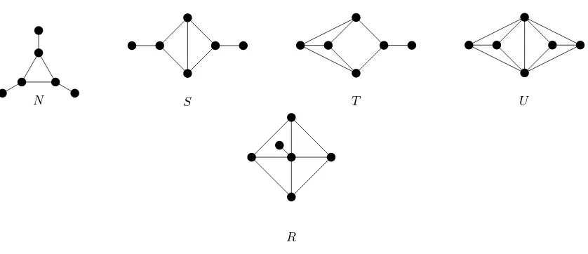
Let H be the set of fourteen graphs shown in Figure 3. In this section, we establish the following theorem:
Theorem 11 The set Odh is equal to the set H.
It is not difficult to verify that each of the graphs in Figure 3 is a member ofOdh.
Lemma 12 H is a subset ofOdh.
Proof.By observation, each graphGinHhas lrw(G)>1. One can not start at any vertex
and visit the other vertices sequentially while keeping width 1. However, after removing any vertex from each graph G, a consistent threading of the remaining graph as a thread
graph can be found.
In the remainder of this section we complete the proof of Theorem 11, showing thatH is the complete set of graphs in Odh.
A graph inOdh is a connected distance-hereditary graph by Lemma 3. Any connected
distance-hereditary graph G of more than one vertex can be described as G=⊕x(G′, u),
where ⊕x is one of the three dh-operations applied to vertex u of a distance-hereditary
graph G′.
Lemma 13 If a distance-hereditary graphG=⊕x(G′, u) is in Odh thenG′ is a connected
thread graph.
Proof.Since G is a minimal forbidden induced subgraph, the graphG′ in any construction must have linear rank-width less than or equal to 1. Graph G′
must be connected, as the
distance hereditary operations maintain connectivity.
Throughout this section, let graph G be ⊕x(G′, u), where G′ is a distance-hereditary
graph, as described above. To discover all distance-hereditary obstructions to linear rank-width 1, we consider each of the three dh-operations applied to all possible cases for vertex uof a thread graphG′. We show that after applying the operation, we have either a thread graph G or a graph G that is one of the 14 graphs of Figure 3 (in set H) as an induced subgraph. First, we consider applying a dh-operation to a thread vertex uof G′.
Lemma 14 Applying any one of the three dh-operations to a non-bridging thread vertex u∈V(G′
) results in a thread graph.
Proof.Assume wlog. that the non-bridging thread vertexuis at the right end of a consistent
Q T X
S V U
N R P W
[image:10.612.102.478.153.523.2]S0 S1 S2 S3
Lemma 15 Applying⊕p(G′, u)whenuis a bridging thread vertex of G′ results in a thread
graph.
Proof. The new vertex v can be considered to be a non-thread vertex labeled “L” (“R”)
as the first (last) vertex in the thread block sequence in one of the two consecutive thread
blocks of which vertex u is a member.
Lemma 16 Applying⊕f(G′, u)or⊕t(G′, u)whenuis a bridging thread vertex ofG′results
in a non-thread graph G containing Q, S, T, U, V, or X (shown in Figure 3) as an induced subgraph.
Proof.Choose a consistent threading ofG′
. By Remark 7,uis a bridging vertex ofG′ with respect to this threading. Hence uhas two neighbors, u1 and u2, that are thread vertices.
If both u1 andu2 are bridging vertices as well, then⊕f(G′, u) contains the half-cubeQas
an induced subgraph, and⊕t(G′, u) containsS as an induced subgraph.
If a neighbor, sayu1 is not bridging, butu2 is bridging, then the thread block involving
u1is non-trivial, so eitheru1 has a pendant vertex oru1 andushare a common neighbor. If
u1 has a pendant vertex, then⊕f(G′, u) containsQas an induced subgraph, and⊕t(G′, u)
containsS as an induced subgraph. Ifu1 and u share a common neighbor, then ⊕f(G′, u)
containsT as an induced subgraph and⊕t(G′, u) containsV as an induced subgraph.
If both u1 and u2 are non-bridging, then G′ has exactly two thread blocks and both
thread blocks are non-trivial. If both u1 and u2 have pendant vertices, then ⊕f(G′, u) is
isomorphic toQand⊕t(G′, u) is isomorphic toS. Ifu1 has no pendant vertex, butu2has a
pendant vertex, then we find that⊕f(G′, u) is isomorphic toT and⊕t(G′, u) is isomorphic
toV. Finally, if neitheru1 noru2 has a pendant vertex, then⊕f(G′, u) is isomorphic toX
and ⊕t(G′, u) is isomorphic toU.
What remains is to consider the cases for dh-operation⊕xbeing applied to a non-thread
vertex u of G′
. Assume a given consistent threading of the thread block containing u in the thread graph G′.
We consider the following cases for non-thread vertexu, depending on the structure of the thread block containing u.
1.L(u) =“∗”
1.1uhas neither a bridging thread vertex nor a non-thread vertex labeled “L” or “R” before it (the case for “after” is symmetric)
1.2 u has a bridging thread vertex or a non-thread vertex labeled “L” or “R” both before and after it
2.L(u) =“R” (the case for L(u) =“L” is symmetric)
2.1 u has no vertex labeled “L” or “∗” after it (i.e., u is a pendant vertex) 2.1.1u is adjacent to a non-bridging thread vertex
2.1.2u is adjacent to a bridging thread vertex
2.2.1u has neither a bridging thread vertex nor a non-thread vertex labeled “∗” or “L” before it
2.2.2 u has a bridging thread vertex or a non-thread vertex labeled “∗” or “L” before it
We must consider the three dh-operations applied in each of these structural cases. We refer to the above numbering of cases in the lemmas to follow.
Lemma 17 (Case 1.) Applying⊕t(G′, u)whenu is a non-thread vertex labeled “∗” inG′
results in a thread graph G.
Proof.The new vertexvcan have the same label and be consecutive withu in a consistent
threading ofG.
Lemma 18 (Case 1.1) Applying ⊕p(G′, u) or ⊕f(G′, u) when u is a non-thread vertex
labeled “∗” that has neither a bridging thread vertex nor a non-thread vertex labeled “L” or “R” before it results in a thread graph G.
Proof. The vertex u can become the thread vertex at the left end of the thread block. A
consistent threading of G will include the new vertex v as the first vertex of the thread block sequence, labeled “L” in the pendant vertex case or “R” in the false twin case.
Lemma 19 (Case 1.2) Applying ⊕p(G′, u) or ⊕f(G′, u) when u is a non-thread vertex
labeled “∗” that has a bridging thread vertex or non-thread vertex labeled “L” or “R” before and after it results in a non-thread graph G that has graph N, R, P, or W shown in Figure 3 as an induced subgraph.
Proof.Note that the case that uhas a bridging vertexv before it is subsumed by the case
that it has a pendant vertex labeled “L” before it. Vertexv is part of a thread edge of the adjacent thread block, connecting it to another thread vertexw. Deleting all vertices other thanv andw of that adjacent thread block yields the case whereuhas a vertex wlabeled “L” before it. The case whereu has a bridging vertex after it is similarly subsumed by the case that it has a vertex labeled “R” after it.
First, consider the cases of applying operation⊕p(G′, u). If u has a vertex labeled “L”
before it and a vertex labeled “L” after it, applying⊕p(G′, u) results in a graph containing
induced subgraph P. The result is the same if u has a vertex labeled “R” before it and a vertex labeled “R” after it. Ifu has a vertex labeled “L” before it and a vertex labeled “R” after it, applying ⊕p(G′, u) results in a graph Gcontaining induced subgraph N. Finally,
ifuhas a vertex labeled “R” before it and a vertex labeled “L” after it, applying⊕p(G′, u)
results in a graphG containing induced subgraphR.
Now, consider the cases of applying operation⊕f(G′, u). If u has a vertex labeled “L”
before it and a vertex labeled “L” after it, applying⊕f(G′, u) results in a graph containing
vertex labeled “R” after it. Ifu has a vertex labeled “L” before it and a vertex labeled “R” after it, applying ⊕f(G′, u) results in a graph G containing induced subgraph P. Finally,
ifuhas a vertex labeled “R” before it and a vertex labeled “L” after it, applying ⊕f(G′, u)
results in a graphG containing induced subgraphW.
Now, consider Case 2, a non-thread vertex ulabeled “R” in G′.
Lemma 20 (Case 2.) Applying ⊕f(G′, u) when u is a non-thread vertex labeled “R” in
G′
results in a thread graph G.
Proof. The vertex v can have the same label and be consecutive with u in a consistent
threading of G.
Consider Case 2.1 whereuis a pendant vertex of G′. In these cases, u is adjacent to a thread vertex wof G′
.
Lemma 21 (Case 2.1.1) Applying⊕p(G′, u) or ⊕t(G′, u) when u is a pendant vertex in
G′
labeled “R” adjacent to a non-bridging thread vertex w results in a thread graph G.
Proof.The vertexuwill become a thread vertex (with vertexwbecoming a bridging thread
vertex) in a consistent threading of thread graph G.
Lemma 22 (Case 2.1.2) Applying⊕p(G′, u) or ⊕t(G′, u) when u is a pendant vertex in
G′ labeled “R” adjacent to a bridging thread vertex w results in a graph G having S
0, S1,
S2, or S3 of Figure 3 as an induced subgraph.
Proof. The vertex w would become a bridging vertex in G = ⊕x(G′, u) shared by three non-trivial thread blocks, contradicting the property of a thread graph of Remark 7. The minimal, non-trivial thread graphs with two thread blocks are given by Lemma 9; these minimal graphs determine the obstruction set generated by the operation.
Finally, consider Case 2.2, when u is labeled “R” and is in a 4-cycle, having a vertex labeled “L” or “∗” after it in the thread block.
Lemma 23 (Case 2.2.1) Applying⊕p(G′, u)or⊕t(G′, u)to a non-thread vertexulabeled
“R” that is in a 4-cycle and has neither a bridging thread vertex nor a non-thread vertex labeled “∗” or “L” before it results in a thread graphG.
Proof.In this case, the left thread vertex of the block is an end vertex on the thread. This
case is as that discussed in Lemma 14; vertex u can “switch places” with the original left
thread vertex of the thread block.
Lemma 24 (Case 2.2.2) Applying⊕p(G′, u) or ⊕t(G′, u) to non-thread vertex u labeled
or “L” before it results in a graph G having one of the graphs Q, S, T, V, X, or U of Figure 3 as an induced subgraph.
Proof.Note that the case that uhas a bridging vertexv before it is subsumed by the case
that it has a pendant vertex labeled “L” before it. Vertexv is part of a thread edge of the adjacent thread block, connecting it to another thread vertexw. Deleting all vertices other thanv andw of that adjacent thread block yields the case whereuhas a vertex wlabeled “L” before it.
First, consider the cases where operation⊕p(G′, u) is applied. If there is a vertex labeled
“L” before u, thenG contains induced subgraphQ orS depending on whether the vertex following u is labeled “L” or “∗”, respectively. If there is a vertex labeled “∗” before u, thenGcontains induced subgraph T orV depending on whether the vertex followingu is labeled “L” or “∗”, respectively.
Now, consider the cases where operation⊕t(G′, u) is applied. If there is a vertex labeled
“L” beforeu, thenGcontains induced subgraphT orV depending on whether the vertex following u is labeled “L” or “∗”, respectively. If there is a vertex labeled “∗” before u, thenGcontains induced subgraphX orU depending on whether the vertex followingu is
labeled “L” or “∗”, respectively.
Proof of Theorem 11.By Lemma 12,His a subset ofOdh. There can be no further members
ofOdh as the above lemmas cover all possible cases of applying a dh-operation to a thread
graph. The set of non-thread graphs that results from these cases is exactly equal to set
H. ⊓⊔
Proof of Theorem 4. The proof follows from Theorem 11 and Lemma 6. ⊓⊔
5 Vertex-Minor Obstructions
Let G be a graph and let v ∈ V(G). The graph obtained from G by performing a lo-cal complementation at v is the graph G∗v with V(G∗v) := V(G) and E(G∗v) := E(G)∆
{x, y} ⊆ NG(v)
x 6= y (∆ denoting the symmetric difference of two sets). We say that two graphs Gand H arelocally equivalent, ifH can be obtained fromGby a se-quence of local complementations. Note that this is indeed an equivalence relation. Figure 4 shows all graphs that are locally equivalent to C5 (up to isomorphism).
A graphH is avertex-minor of a graphG, ifH can be obtained from Gby a sequence of local complementations and vertex deletions. In particular, every induced subgraph ofG is a vertex-minor of G.H is aproper vertex-minor of G, ifH 4v Gand |V(H)|<|V(G)|.
For a given, non-negative integer k, the class of graphs of rank-width at mostk is closed under taking of vertex-minors [14].
C5
[image:15.612.200.451.92.178.2]“house” “gem”
Figure 4.The three graphs that are locally equivalent toC5.
[image:15.612.172.482.231.318.2]C5 N Q
Figure 5. The three vertex-minor obstructions for linear rank-width at most 1: The 5-cycleC5, the net graphN, and the half-cubeQ.
Theorem 25 The vertex-minor obstructions for the class of graphs of linear rank-width at most 1 are the three graphs C5,N and Q depicted in Figure 5.
Proof. Since the class of graphs of linear rank-width at most 1 is closed under taking
vertex-minors, it suffices to show that the graphs in Figure 5 are a set of pairwise not locally equivalent obstructions, such that every graph with linear rank-width at least 2 contains one of them as a vertex-minor. Indeed, it is not hard to see that the graphs in Figure 5 are pairwise not locally equivalent.
Every graphGwith linear rank-width≥2 contains one of the graphs listed in Theorem 4 as an induced subgraph.
IfGcontains a hole, the house, the gem or the domino graph, then it contains C5 as a
vertex-minor: Any cycleCk, withk >5, can be reduced in size by repeatedly performing a
local complementation and deleting the degree 2 vertex of the resultant 3-cycle. Applying local complementation to a vertex of C5 yields the house graph. Applying local
comple-mentation to one of mutually adjacent vertices of degree 2 of the house graph yields the gem graph. These locally equivalent graphs are shown in Figure 4. Applying local comple-mentation to any vertex v of the domino graph (see Figure 8) and then deletingv, yields a graph locally equivalent to the C5. Thus, the only non-distance-hereditary vertex-minor
To determine the set of distance-hereditary vertex-minor obstructions, first consider the induced subgraph obstructionsS0,S1,S2,S3 that are created by Lemma 22 (shown in
Figure 3). All four of these graphs have the net graphN as a vertex-minor. This is realized by first applying local complementation to a vertex of degree 2 in any triangle, reducing all four graphs toS0. By applying local complementation to the central vertexv of degree
3 in S0 and then deleting v, one realizes the net graphN.
Figure 6 and Figure 7 show the remaining ten induced subgraph obstructions postu-lated by Theorem 11 grouped by local equivalence with graphs N and Q. By applying local complementation to the bottom vertex of graphS, one reaches N. By applying local complementation to the vertices in triangles on the sides of T and U, one reaches S. By applying local complementation to the degree 5 vertex of graph R, one reaches graph U. For the graphs locally equivalent to Q, applying local complementation to a degree 2 ver-tex ofP yieldsQ. Applying local complementation to the vertex with a pendant neighbor in graph V yields graph X. By applying local complementation to one vertex from each side ofX in succession, one reachesQ. Finally, applying local complementation to the top vertex of graph W yields graphX.
Therefore, by deleting zero or more vertices from any graphGwith lrw(G)≥2, one of the induced subgraph obstructions of Theorem 4 will be encountered. This subgraph can be reduced to one of the three vertex-minor obstructions, as shown above.
N S T U
[image:16.612.80.499.411.592.2]R
Q P V
[image:17.612.162.491.88.273.2]X W
Figure 7.The five induced subgraph obstructions locally equivalent to the half-cubeQ.
6 Pivot-Minor Obstructions
Pivot-equivalence is defined with respect to an edge {u, v}. Define three sets of vertices A, B, and C as A = {w|{u, w} ∈ E(G) and {v, w} ∈/ E(G)}, B = {w|{u, w} ∈ E(G) and {v, w} ∈ E(G)}, C = {w|{u, w} ∈/ E(G) and {v, w} ∈ E(G)}. The result of a pivot operation G× {u, v} is defined as the complementation of edges of G between the three sets of vertices A, B, and C, and also between{u, v}and A∪C (“swappingu and v”).
We say that two graphs, Gand H are pivot-equivalent,G∼p H ifH can be obtained
from G by a sequence of pivot operations. Pivot-minor containment, H 4p G, is defined as H being an induced subgraph of any graph pivot-equivalent to G.H is aproper pivot-minor of G, if H 4p G and |V(H)|< |V(G)|. It is easy to check that for an edge {u, v}
in G, G× {u, v} = G∗u∗v∗u. Therefore, pivot-minor containment is a special case of vertex-minor containment.
A graphG is apivot-minor obstruction for the class of graphs of linear rank-width at most 1, if lrw(G)≥2 and every proper pivot-minorH of Gsatisfies lrw(H)≤1.
[image:17.612.281.367.544.596.2]Theorem 26 The pivot-minor obstructions for the class of graphs of linear rank-width at most 1 are the eight graphs depicted in Figure 9.
Proof. We define C+
k, for k > 5, as the cycle on k vertices with a chord between two
vertices at distance 3 along the cycle. Figure 8 showsC6+, the domino graph. By applying the pivot operation to an edge between two vertices of degree 2, one sees that Ck ∼p Ck+
and therefore, for all k > 6, Ck−2 4p Ck. As a result, all non-distance-hereditary graphs
contain C5 orC6 as a pivot-minor; these graphs are the two pivot-minor obstructions for
the class of distance-hereditary graphs [2].
Now consider the induced subgraph obstructionsSi, for 0≤i≤3. By applying the pivot
operation to an edge that includes the central vertex of one of these graphs, a graph that contains another obstruction as an induced subgraph is generated. For example, applying the pivot operation to such an edge in S0 and then deleting the non-central vertex of the
edge results in obstructionQ. Similarly,S1 results in obstructionT,S2results inX, andS3
results inU. Therefore, the induced subgraph obstructionsSiare eliminated as pivot-minor
obstructions.
To determine the remaining pivot-minor obstructions for the class of graphs with linear rank-width at most 1, we need only identify pivot-equivalent graphs in Odh. One finds
that N ∼p R, S ∼p T, P ∼p W, X ∼p V. There are no further equivalences among these
graphs, that would allow reduction of this set of graphs. This can be established readily, by observation, as there are few distinct edges in each proposed obstruction. For example, consider graph N. Applying a pivot operation to a pendant edge results in the identical graph. Applying the pivot operation to the other distinct edge of N, results in graph R. Applying the pivot operation to the pendant edge of R results in R. Applying the pivot operation to an edge between two vertices of degree 3 results in graphN, Applying the pivot operation to the other edge inR results in a graph isomorphic toR. A similar case analysis shows that applying the pivot operation to edges of any of the other pivot-equivalent pairs of graphs inOdh that were noted above only results in graphs isomorphic to graphs of the
pair.
7 Conclusion
C5 C6
N S U
[image:19.612.163.486.89.358.2]Q P X
Figure 9.The eight pivot-minor obstructions for linear rank-width at most 1.
would be to determine the obstruction set for the graphs of linear rank-width at most 2. However, we expect the number of obstructions to be large.
8 Acknowledgement
We thank the anonymous referees for their careful scrutiny of our manuscript; their com-ments helped us to provide a clearer exposition of our results.
References
1. Isolde Adler and Mamadou M. Kant´e. Linear rank-width and linear clique-width of trees, 2013. WG’13, Accepted.
2. Hans-J¨urgen Bandelt and Henry Martyn Mulder. Distance-hereditary graphs. J. Comb. Theory, Ser. B, 41(2):182–208, 1986.
3. Hans L. Bodlaender. A partialk-arboretum of graphs with bounded treewidth. Theor. Comput. Sci., 209(1-2):1–45, 1998.
4. Andr´e Bouchet. Circle graph obstructions. J. Comb. Theory, Ser. B, 60(1):107–144, 1994.
6. Bruno Courcelle and Stephan Olariu. Upper bounds to the clique width of graphs. Discrete Applied Mathematics, 101(1-3):77–114, 2000.
7. Reinhard Diestel. Graph minors 1: A short proof of the path-width theorem.Combinatorics, Probability & Computing, 4:27–30, 1995.
8. Wolfgang Espelage, Frank Gurski, and Egon Wanke. How to solve np-hard graph problems on clique-width bounded graphs in polynomial time. In Andreas Brandst¨adt and Van Bang Le, editors,WG, volume 2204 ofLecture Notes in Computer Science, pages 117–128. Springer, 2001.
9. Robert Ganian. Thread graphs, linear rank-width and their algorithmic applications. In Costas S. Iliopoulos and William F. Smyth, editors,IWOCA, volume 6460 ofLecture Notes in Computer Science, pages 38–42. Springer, 2010.
10. Robert Ganian and Petr Hlinen´y. Better polynomial algorithms on graphs of bounded rank-width. In Jir´ı Fiala, Jan Kratochv´ıl, and Mirka Miller, editors, IWOCA, volume 5874 of Lecture Notes in Computer Science, pages 266–277. Springer, 2009.
11. Edward Howorka. A characterization of distance-hereditary graphs. The Quarterly Journal of Mathe-matics, 2(28):417–420, 1977.
12. Nancy G. Kinnersley and Michael A. Langston. Obstruction set isolation for the gate matrix layout problem. Discrete Applied Mathematics, 54(2-3):169–213, 1994.
13. Daniel Kobler and Udi Rotics. Edge dominating set and colorings on graphs with fixed clique-width.
Discrete Applied Mathematics, 126(2-3):197–221, 2003.
14. Sang-il Oum. Rank-width and vertex-minors. J. Comb. Theory, Ser. B, 95(1):79–100, 2005. 15. Sang-il Oum. Rank-width and well-quasi-ordering. SIAM J. Discrete Math., 22(2):666–682, 2008. 16. Sang-il Oum and Paul D. Seymour. Approximating clique-width and branch-width. J. Comb. Theory,
Ser. B, 96(4):514–528, 2006.