Inner functions and operator theory

(1)

White Rose Research Online URL for this paper:

http://eprints.whiterose.ac.uk/84995/

Version: Published Version

Article:

Chalendar, I, Gorkin, P and Partington, JR orcid.org/0000-0002-6738-3216 (2015) Inner

functions and operator theory. North-Western European Journal of Mathematics, 1. pp.

9-28.

(c) The Authors 2015. Published by North-Western European Journal of Mathematics.

Reproduced in accordance with the publisher's contract licence.

(http://math.univ-lille1.fr/~nwejm/#Policies)

[email protected] Reuse

Items deposited in White Rose Research Online are protected by copyright, with all rights reserved unless indicated otherwise. They may be downloaded and/or printed for private study, or other acts as permitted by national copyright laws. The publisher or other rights holders may allow further reproduction and re-use of the full text version. This is indicated by the licence information on the White Rose Research Online record for the item.

Takedown

If you consider content in White Rose Research Online to be in breach of UK law, please notify us by

(2)

North-Western European Journal of Mathematics

Inner functions and operator theory

Isabelle Chalendar1 _{Pamela Gorkin}2 _{Jonathan R. Partington}3

Received: December 7, 2014/Accepted: March 6, 2015/Online: April 2, 2015

Abstract

This tutorial paper presents a survey of results, both classical and new, link-ing inner functions and operator theory. Topics discussed include invariant subspaces, universal operators, Hankel and Toeplitz operators, model spaces, truncated Toeplitz operators, restricted shifts, numerical ranges, and interpola-tion.

Keywords:inner functions, invariant subspaces, universal operators, Hankel and Toeplitz operators, model spaces, interpolation.

msc: 47A15, 47B35, 30H10, 30E05.

1 Introduction

Inner functions originally arose in the context of operator theory, via Beurling’s theorem on the invariant subspaces of the unilateral shift operator. Since then, they have been seen in numerous contexts in the theory of function spaces. This tutorial paper surveys some of the many ways in which operators and inner functions are linked: these include the invariant subspace problem, the theory of Hankel and Toeplitz operators and the rapidly-developing area of model spaces and the operators acting on them.

The paper is an expanded version of a mini-course given at the Eleventh Ad-vanced Course in Operator Theory and Complex Analysis, held in Seville in June 2014.

1.1 Hardy spaces and shift-invariant subspaces

All our spaces will be complex. We writeDfor the open unit disc inCandT=∂D,

the unit circle.

1_{Université Lyon 1, INSA de Lyon, École Centrale de Lyon, CNRS, UMR 5208, Institut Camille}

Jordan, 43 bld. du 11 novembre 1918, F-69622 Villeurbanne Cedex, France

(3)

Recall that Hardy spaceH2orH2(D) is the space of analytic functions onD

with square-summable Taylor coeffi_{cients; that is,}

H2(D) =

      

f :D_→Canalytic,f(z) =X∞

n=0

a_nzn,_kf_k2=X∞

n=0

|a_n_|2<_∞

       .

AlsoH2(D) embeds isometrically as a closed subspace ofL2(T) via

∞

X

n=0

a_nzn7→

∞

X

n=0

a_neint_,

where the series converges almost everywhere onTas well as in the norm ofL2(T).

Indeed, limr→1−f(re

i_t

) exists almost everywhere and gives the boundary values of a functionf inH2(D). (See, for example Hoff_{man (1962).)}

It is useful to use the isometric isomorphismℓ2(Z)_→L2(T) given by

(a_n)_n∈Z7→

∞

X

n=−∞ a_neint_,

which is a consequence of the Riesz–Fischer theorem; this restricts to an isomor-phismℓ2(Z+)→H2(D).

The first connection between inner functions and operator theory arises on considering the right shiftR:ℓ2(Z)_→ℓ2(Z). We may ask what its closed invariant

subspaces are; that is, the subspaces_{M ⊂}L2(T) such thatR_{M ⊂ M}. The answer is to look at the unitarily equivalent operatorSof “multiplication byz” onL2(T).

ℓ2(Z) _{−−−−−−→}R ℓ2(Z)

     y      y

L2(T) _{−−−−−−→}S L2(T)

There are two cases, for_Ma nontrivial closed subspace ofL2(T):

1. SM=M, if and only if there is a measurable subsetE⊂Tsuch that_M=_{f ∈

L2(T) :f_|T_\E= 0 a.e.}(Wiener4).

2. S_M(_M, if and only if there is a unimodular functionφ_∈L∞₍_T_{) such that}

M=φH2(Beurling–Helson5_).

As a sketch proof of item 2, which will be the more important for us, take

φ∈ M ⊖SMwithkφk2= 1. One can verify thatφis unimodular and thatM=φH2.

(4)

1. Introduction

Corollary 1 (Beurling’s theorem6,7_{) –} _Let_M_{be a nontrivial closed subspace of}_H2_;

then SM ⊂ Mif and only if M =θH2 whereθ is inner, that isθ ∈ H2(D) with

|θ(eit)_|= 1_a.e.

It is easily seen thatθis unique up to multiplication by a constant of modulus 1. Now, any functionh∈H2, apart from the zero function, has a multiplicative factorizationh=θu, whereθis inner, anduisouter: Beurling showed that outer functions satisfy

spann

u, Su, S2u, S3u, . . .o=H2,

and they therefore have an operatorial interpretation, as cyclic vectors for the shift

S. The inner-outer factorization is unique up to multiplication by a constant of modulus one.

1.2 Examples of inner functions

IfMis a shift-invariant subspace of finite codimension, thenθis a finite Blaschke product,

θ(z) =λ n

Y

j=1

z−α_j

1−αjz ,

with|λ|= 1 andα1, . . . , αn∈D. Then

M=nf _∈H2:f(α1) =···=f(αn) = 0

o

,

with the obvious interpretation in the case of non-distinctαj. We may also form

infinite Blaschke products

θ(z) =λzp ∞

Y

j=1

|α_j|

α_j α_j−z

1−α_jz,

where|λ|= 1, all theα_jlie inD_\{0_},pis a non-negative integer andP_∞

j=1(1−|αj|)<∞.

Recall that the sequences ofD satisfying the last condition are called Blaschke

sequences.

There is also a class of inner functions without zeroes, namely the singular inner functions, which may be written as

θ(z) = exp

"

−

Z π

−π eit+_z ei_t

−zdµ(t)

#

,

6_{Beurling, 1949, “On two problems concerning linear transformations in Hilbert space”.}

7_{See also Garnett, 2007,}_{Bounded analytic functions}_{, theorem II.7.1; Nikolski, 2002,} _Operators,

(5)

whereµis a singular positive measure on [−π, π). For example ifµis a Dirac mass at 0, thenθ(z) = exp((z+ 1)/(z−1)).

A complete description of inner functions is now available, as they are given as

Bs, whereBis a Blaschke product andsis a singular inner function. Either factor may be absent.

Note that ifθ₁andθ₂are inner, thenθ₁θ₂is unimodular onT. These are not

all the unimodular functions, but ifφ_∈L∞₍_T_{) is unimodular then for each}_{ε >}₀

it can be factorized asφ=h₁h₂, withh₁, h₂_∈H∞_and_k_h₁_k_,_k_h₂_k_<_{1 +}_ε8_{. Related to}

this is the Douglas–Rudin theorem that the quotientsθ1θ2withθ1andθ2inner are

uniformly dense in the unimodular functions inL∞₍_T₎9_.

Of particular importance are the interpolating Blaschke products: a Blaschke productBwith zeroes (z_j) is interpolating if its zero sequence is an interpolating sequence forH∞or, equivalently, there existsδ >0 such that

inf

k

Y

j:j,k

z_j₋z_k

1−z_kz_j

=δ.

These Blaschke products play an important role in the study of bounded analytic functions: consider a closed subalgebraBofL∞_containing_H∞_{properly. In}

estab-lishing a conjecture of R. G. Douglas, Chang; Marshall10_{proved that such algebras}

(now called Douglas algebras) can be characterized using interpolating Blaschke products: if

U_B=n

b:binterpolating andb−1_∈Bo,

then an algebra is a Douglas algebra if and only if it is the closed algebra generated byH∞ _{and the conjugates of the functions in}_U

B. In other words,B= [H∞, UB].

Much more is known about interpolating Blaschke products: in particular, Jones11

showed that one can take the Blaschke products in the Douglas–Rudin theorem to be interpolating. Related work can be found in Marshall and Stray (1996), Garnett and Nicolau (1996), and Garnett (2007). One very interesting question remains open: can every Blaschke product be approximated (uniformly) by an interpolating Blaschke product Hjelle and Nicolau12_{have shown that given a Blaschke product,}

B, there is an interpolating Blaschke product that approximatesBin modulus onD,

but this is the best result to date.

8_{Bourgain, 1986, “A problem of Douglas and Rudin on factorization”;}

Barclay, 2009, “A solution to the Douglas-Rudin problem for matrix-valued functions”; Chalendar and Partington, 2011,Modern approaches to the invariant-subspace problem. 9_{Douglas and Rudin, 1969, “Approximation by inner functions”.}

10_{Chang, 1976, “A characterization of Douglas subalgebras”;} Marshall, 1976, “Subalgebras ofL∞containingH∞”. 11_{Jones, 1981, “Ratios of interpolating Blaschke products”.}

(6)

2. Some operators associated with inner functions

2 Some operators associated with inner functions

2.1 Isometries

1. It is not hard to see that theanalytic Toeplitz operatoror Laurent operator,

T_φ:H2→H2,f 7→φf, whereφ∈H∞_{, is an isometry if and only if}_φ_{is inner.}

Moreover codimφH2<∞if and only ifφis a finite Blaschke product.

2. Forφ:D_→Dholomorphic, we may consider thecomposition operatorC_φ:

H2→H2,f 7→f ◦φ. See for example Cowen and MacCluer (1995) for full details on these. In particular, by Littlewood’s subordination theorem13_,_C

φis

automatically continuous.

It is a result of E. A. Nordgren14_that_C

φis an isometry if and only ifφis inner

andφ(0) = 0. Note that ifφis inner, withφ(0) = 0, then forn > mwe have

hφn, φm_i=_hφn−m,1_i=φ(0)n−m_{= 0}_,

so that the orthonormal sequence (zn)n≥0 in H2 is mapped to the orthonormal

sequence (φn)n≥0.

Conversely, since hz,1i= 0, we must haveφ(0) =hφ,1i= 0 if Cφ is to be an

isometry. Also the condition_kφnk= 1 for allncan be used to check thatφis inner.

Bayart15 _{shows that}_C

φ issimilarto an isometry if and only ifφis inner and φ(p) =pfor somep_∈D.

2.2 Universal operators

An operatorU defined on a separable infinite-dimensional Hilbert spaceHis said to beuniversalin the sense of Rota, if for every operatorT on a Hilbert space_K there is a constantλ_∈Cand an invariant subspace_MforU such thatT is similar to the restrictionλU_|M.

H −−−−−−→

λU H

x     

M −−−−−−→

λU M

J

    

y J

     y

K −−−−−−→

T K

13_{Littlewood, 1925, “On inequalities in the theory of functions”.} 14_{E. A. Nordgren, 1968, “Composition operators”.}

(7)

The following theorem provides many examples of universal operators.

Theorem 1 (Caradus16) – If the operatorU:_{H → H}is surjective with infinite-dimen-sional kernel, then it is universal.

1. Takeθinner, but not a finite Blaschke product. Then using Theorem theorem 1 one can show that the Toeplitz operatorT_θ=T_θ∗:H2→H2, withf 7→P_H2(θf)

is universal.

Such an operatorT_θ∗ is similar to the backward shiftAonL2(0,∞), given by

Af(t) =f(t+ 1),

which by the Laplace transform is unitarily equivalent to the adjoint of the operator Me−s of multiplication of e−s on the Hardy spaceH2(C+) of the

right half-plane C₊ (heres is the independent variable). Note thate−s is inner: still, in spite of Beurling’s theorem mentioned above, there is no usable characterization of the invariant subspaces ofA.

2. Letφ:D_→Dbe defined by

φ(z) =z+ 1/2 1 +z/2;

this is a (hyperbolic) automorphism fixing_±1. The composition operatorC_φ

has spectrum given by

σ(C_φ) =n

z∈C: 1/√3≤ |z| ≤√3o

.

Forλ_∈intσ(C_φ), it can be shown thatC_φ₋λI is universal17_{. Note that it}

has the same invariant subspaces asC_φ, and a complete description of them would give a solution to the invariant subspace problem.

These ideas have stimulated studies on cyclic vectors and minimal invariant subspaces forC_φ(e.g. Mortini (1995) and Gallardo-Gutiérrez and Gorkin (2011)).

2.3 Hankel and Toeplitz operators

We begin with the orthogonal decomposition

L2(T) =H2⊕H₀2

into closed subspaces spanned by{eint:_n_≥0_}and_{eint:_{n <}0_}, respectively. Write P:L2(T)_→H2for the orthogonal projection.

16_{Caradus, 1969, “Universal operators and invariant subspaces”.}

(8)

2. Some operators associated with inner functions

Definition 1 – Letφ∈L∞(T). Then theToeplitz operatorT_φ:H2→H2is defined byT_φf =P(φf) for f _∈ H2. The Hankel operator Γ

φ : H2 → H02 is defined by Γ

φf = (I−P)φf forf ∈H2.

It is well known that_kT_φ_k=_kφ_k_∞18and that_kΓ

φk= dist(φ, H∞)19.

2.4 Kernels

1. If u ∈kerΓ_φ, then _φu _∈ _H2, so that_zφu_∈ _H2 and_zu _∈ kerΓ_φ. Hence, by

Beurling’s theorem, kerΓ

φ=θH2for some inner functionθ.

For example, if θ is inner, thenu ∈ kerΓ

θ if and only ifθu ∈ H2, which

happens if and only ifu _∈θH2. So all Beurling subspaces occur as Hankel kernels.

2. Suppose thatθis inner. Thenf ∈kerT_θif and only ifhθf , gi= 0 for allg∈H2. This is equivalent to the conditionhf , θgi= 0; that is,f ∈H2⊖θH2. We shall study these spaces in Section section 3 on the following page.

Toeplitz kernels in general have thenear-invarianceproperty. Ifu _∈H2 and

θu ∈kerT_φ for some inner functionθ, thenφθu =zh for someh∈ H2. Hence

φu=θzhand thusu∈kerT_φ.

That is, ifv∈kerTφandv/θ∈H2, thenv/θ∈kerTφ.

In particular, ifv_∈kerT_φandv/z_∈H2, thenv/z_∈kerT_φ. This property is not the same as beingS∗-invariant, even thoughS∗v=v/zifv/z∈H2.

For example, letφ(z) =e−z_/z2. One may verify that

kerT_φ=_{(a+bz)ez:_{a, b}_∈_C_}_.

HoweverS∗ez=ez−1

z , which does not lie in kerTφ.

Now Hitt20_{showed that a subspace}_{M ⊂}_H2_{is nearly}_S∗_{-invariant if and only if}

it can be written as_M=f K_θ, whereθis inner,θ(0) = 0,f _{∈ M ⊖}(_{M ∩}zH2), and

K_θis the model spaceH2_⊖θH2, discussed in Section section 3 on the next page. Moreover, Hayashi; Hayashi21_{showed that such an}_M_{is in fact a Toeplitz kernel}

if and only if the functionf has the property thatf2isrigid, which means that if

g∈H1withg/f2>0 a.e., theng=λf2for some constantλ >0. A rigid function is necessarily outer.

18_{Brown and Halmos, 1963, “Algebraic properties of Toeplitz operators”.} 19_{Nehari, 1957, “On bounded bilinear forms”.}

20_{Hitt, 1988, “Invariant subspaces of}_H2_{of an annulus”.} 21_{Hayashi, 1986, “The kernel of a Toeplitz operator”;}

(9)

3 Model spaces

3.1 Definitions and examples

Since the invariant subspaces forShave the formθH2, withθinner, those forS∗

have the formH2⊖θH2, usually writtenK_θ. Such spaces are calledmodel spaces.

Example 1 –

1. Takeθ(z) =zN_{, which is inner. Then}

K_θ= spann

1, z, z2, . . . , zN−1o.

2. Forθ(z) =QN

k=11z−α−αkkz withα1, . . . , αNdistinct, we havef ∈θH

2_{if and only if}

f(α1) =···=f(αN) = 0. Then

Kθ= span

(

1 1−α1z, . . . ,

1 1−α_Nz

)

.

Indeed, forα_∈D,k_α:z_7→₁₋1_αz is thereproducing kernelatα; i.e.,

f(α) =hf , kαi for f ∈H2,

and clearlyf ∈θH2if and only iff is orthogonal tok_α₁, . . . , k_α_N.

3. For a fixedτ >0 we write

L2(0,_∞) =L2(0, τ)_⊕L2(τ,_∞). (1)

Under the Laplace transform this maps to the orthogonal decomposition

H2(C₊) =K_θ_⊕θH2(C₊),

whereθ(s) =e−sτ; that is,_θis inner. Then_K

θcan be written asesτ/2PWτ/2,

wherePWτ/2is aPaley–Wienerspace, consisting of entire functions, as

consid-ered in signal processing.

In generalK_θis finite-dimensional if and only ifθis a finite Blaschke product.

3.2 Decompositions of

H

2

and

K

B

Letθbe inner. Then

(10)

3. Model spaces

This is an orthogonal direct sum, since ifk1, k2∈Kθand 0≤m < n, then

hθmk₁, θnk₂_i=_hk₁, θn−mk₂_i= 0,

sincek1⊥θH2.

Note thatT_θacts as a shift here, i.e.,

θ(k1+θk2+θ2k3+···) =θk1+θ2k2+θ3k3+···

A special case of this can be identified from equation (1) on page 16, since

L2(0,∞) =L2(0, τ)⊕L2(τ,2τ)⊕ ···

We now look at model spaces corresponding to infinite Blaschke products. Ifα1, α2, . . .are the zeroes of an infinite Blaschke product B(assumed distinct),

then an orthonormal basis ofKBis the Takenaka–Malmquist–Walsh basis given by

orthonormalizing the sequence of reproducing kernels associated with the (αn). We

have

e₁(z) =(1− |α1|2)1/2 1−α1z ,

e2(z) =(1− |α2| 2₎1/2

1₋α₂z

z−α1

1₋α₁z

!

,

and, in general

en(z) =

(1_{− |}α_n_|2)1/2

1−α_nz

      

n−1

Y

k=1

z₋α_k

1−α_kz

      

.

It is easily checked that these are orthonormal, and have the same closed span as the reproducing kernels₁_−α1

1z, . . . ,

1

1−αnz, . . .This closed span isKBwhen the (αn) form a Blaschke sequence, andH2otherwise.

3.3 Frostman’s theorem and mappings between model spaces

The following result shows that inner functions are not far from Blaschke products, in a precise sense.

Theorem 2 (Frostman22_{) –} _Let_θ_{be any inner function. Then, for}_α_∈_D_{, the function}

θ−α

(11)

Note that ifφandθare inner thenφ◦θis also inner (this is not obvious). Here we are considering simplyb◦θwherebis the inner function withb(z) = z−α

1−αz.

Frostman gave a stronger version of his theorem, expressed by saying that the exceptional set has logarithmic capacity zero; however, it is beyond the scope of this work.

Theorem 3 – TheCrofoot transform, defined forα_∈Dby

J_αf =

1− |α|21/2

1−αθ f (f ∈Kθ),

is a unitary mapping fromK_θontoK_b◦θfor each inner functionθ.

In combination with Frostman’s theorem, this can be used to construct orthonormal bases for any model spaceK_θ.

3.4 Truncated Toeplitz and Hankel operators

Truncated Toeplitz operators were introduced by Sarason23_{, and have received much}

attention since then. The idea here is to put finite Toeplitz matrices of the form

           

a0 a−1 . . . a−n a1 a0 . . . a−n+1

. . . . . . . . . . . . a_n a_n−1 . . . a0

            (2)

into a more general context. One may also consider finite Hankel matrices of the form            

a₋₁ a₋₂ . . . a_−n−₁ a₋2 a−3 . . . a−n−2

. . . . . . . . . . . . a_−n−1 a−n−2 . . . a−2n−1

            . (3)

Takeθinner, andφ_∈L∞₍_T_{); then the truncated Toeplitz operator}_Aθ

φ:Kθ→Kθis

defined by

Aθ_φf =P_K_θ(φ·f) (f ∈K_θ),

whereP:L2(T)_→K_θis the orthogonal projection.

22_{Frostman, 1935, “Potentiel d’équilibre et capacité des ensembles avec quelques applications à la} théorie des fonctions”.

(12)

4. Restricted shifts

The motivating example involves the choiceθ(z) =zn+1, and the orthonormal basis{1, z, z2, . . . , zn}ofKθ, when the matrix ofAθ_φhas the form (2), with (an)n∈Zthe

Fourier coefficients of_φ.

Similarly for truncated Hankel operators. The operatorBθ_φ:K_θ→zK_θis defined by

Bθ_φf =P_zK_θ(φ·f) (f ∈Kθ).

Now, ifθ(z) =zn+1_{, then}_zK

θhas basis{z, . . . , zn+1}, and with these bases the operator Bθ_φhas a truncated Hankel matrix (3).

4 Restricted shifts

4.1 Basic ideas

We recall that the invariant subspaces of the backwards shiftS∗have the formKθ.

We now defineSθ:Kθ→Kθby

S_θ=P_K_θS_|K_θ = (S_|K∗

θ)

∗_.

This is the truncated Toeplitz operator with symbolz, and if we takeθ(z) =zn+1it

maps as follows: 1_7→z, z_7→z2, . . . , zn−1_7→_zn_{, z}n_7→_{0, so that its matrix is given by}

                    

0 0 0 . . . 0 0 1 0 0 . . . 0 0 0 1 0 . . . 0 0

. . . .

0 0 0 . . . 0 0 0 0 0 . . . 1 0

                     .

The restricted shift has a part in the Sz.-Nagy–Foias functional model24_{: if}_T

is a contraction on a Hilbert space H such that_k(T∗₎n_x_{k →}_{0 for all} _x_∈_H _and

rank(I−T∗_T_{) = rank(}_I₋_{T T}∗_{) = 1, then there is an inner function}_θ_{such that}_T _is

unitarily equivalent toS_θ.

Proposition 1 – The invariant subspaces for the restricted shiftS_θare “shifted” model spaces of the formK_θ∩φH2 =φK_θ/φ, where φ is an inner function dividing θ in H∞(D).

Proof. The invariant subspaces for its adjoint,S∗

|Kθ are clearly of the formKφ, where

φdividesθinH∞(D). Their orthogonal complements are the invariant subspaces

forS_θ, and have the required form.

(13)

It is easy to see that rankS_θ<∞if and only ifθis a finite Blaschke product. We now define thespectrumof an inner functionθby

σ(θ) =w_∈D: liminf

z→w |θ(w)|= 0

.

For a Blaschke productB, the setσ(B) is the closure of the zero set ofBinD. It can

then be shown that in generalσ(Sθ) =σ(θ)25.

4.2 Unitary perturbations and dilations

We shall now suppose thatθ(0) = 0: this simplifies some of the formulae, but is not a serious restriction. Clark26_{initiated a very fruitful study of unitary perturbations}

of restricted shifts. In particular, he showed that the set of rank-1 perturbations of

S_θthat are unitary can be parametrised as_{U_α:α_∈T_}, where

Uαf =Sθf +αhf , S∗θi1, (f ∈Kθ),

noting that the constant function 1 lies inK_θbecauseθ(0) =hθ,1i= 0.

If we consider the caseθ(z) =zn+1, as above, we find that the matrix ofU_α is now                     

0 0 0 . . . 0 α

1 0 0 . . . 0 0 0 1 0 . . . 0 0

. . . .

0 0 0 . . . 0 0 0 0 0 . . . 1 0

                     ,

so that 1, z, . . . , zn−2_{, z}n−1_{are mapped, respectively, to}_{z, z}2_{, . . . , z}n−1_{, α}_.

The spectral measure of U_α is called a Clark measure, and there are various

applications. See, for example, the book Cima, Matheson, and Ross (2006). For an operatorT on a Hilbert spaceH, we consider the question of finding a unitary operatorU on a space containingH, such that its restriction toHisT. In matrix terms we may write

U = T ∗ ∗ ∗

!

.

IfU is defined onH_⊕C, then we call it a 1-dilation. This is not the same as the

standard Sz.-Nagy–Foias dilation as in Szökefalvi-Nagy et al. (2010). In the context of restricted shifts and unitary dilations, there is a connection here with a classical result in geometry, which we now develop.

25_{Helson, 1964,}_{Lectures on invariant subspaces}_{, Lec. VIII.}

(14)

4.3 Numerical ranges

For an integern≥3, a closed subsetAofDhas then-Poncelet property, if whenever there exists ann-gonPsuch thatPcircumscribesAand has its vertices onT, then

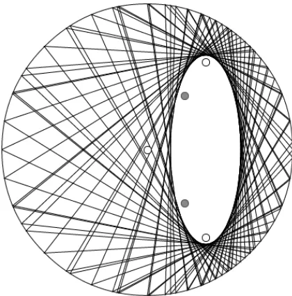
every point on the unit circle is a vertex of such ann-gon. This was originally studied in the context of an ellipse, as in figure 1. (The figures were produced by an applet written by A. Shaff_{er.) Associated with the ellipse is a Blaschke product,}

as we shall explain: its zeroes are denoted by light circles and the zeroes of its derivative by dark circles.

[image:14.482.139.349.216.429.2]

We shall also be considering a generalization of this, namely, an infinite Poncelet property.

Figure 1: Poncelet ellipse with triangles

Let us suppose first thatθis a finite Blaschke product, and henceK_θ is finite-dimensional. Recall that thenumerical rangeof an operatorT on a Hilbert spaceH

is defined by

W(T) =_{hT x, x_i:x_∈H,_kx_k= 1_},

and, according to the Toeplitz–Hausdorff_{theorem, is a convex subset of the plane.}

(15)

Theorem 4 – For the restricted shiftS_θon a finite-dimensional model spaceK_θwe have

W(S_θ) =\

α∈T

W(U_αθ),

where theUθ

α are the rank-1 Clark perturbations ofSzθ, which are equivalent to unitary 1-dilations ofS_θ.

For versions of this results and further developments, see Gau and Wu (1998), Gau and Wu (2003), Gorkin and Rhoades (2008), and Daepp, Gorkin, and Voss (2010).

Note that

σ(U_αθ) ={z∈T:zθ(z) =α},

ann+ 1-point set if the degree ofθisn. Moreover,W(Uθ

α) is the convex hull of σ(Uθ

α), namely, a polygon. If degθ= 2, then it is known thatW(Sθ) is an ellipse,

with foci at the eigenvalues ofS_θ. Therefore, this ellipse has foci at the zeroes ofθ, and it is here expressed as an intersection of triangles.

Figure 2 on the facing page and figure 3 on page 24 show similar examples with

n= 3 (quadrilaterals) andn= 4 (pentagons).

The following more general result was proved in Chalendar, Gorkin, and Part-ington (2009). Note that numerical ranges no longer need to be closed, so the formulation is slightly diff_erent.

Theorem 5 – Letθbe an inner function. Then W(S_θ) =\

α∈T

W(Uαθ),

where the U_αθ are the unitary 1-dilations of S_θ (or, equivalently, the rank-1 Clark perturbations ofS_zθ).

In general we may regard the numerical ranges of theU_αθas convex polygons with infinitely-many sides. Some vectorial generalizations of these results (involving more general contractions) are given in Benhida, Gorkin, and Timotin (2011) and Bercovici and Timotin (2014).

We may now ask how many polygons are needed to determineθuniquely. Note that the vertices of a polygon are solutions tozθ(z) =α, so we are motivated to consider boundary interpolation by inner functions.

4.4 Interpolation questions

(16)

[image:16.482.140.351.75.296.2]

Figure 2: Symmetrical Poncelet curve with quadrilaterals

{z₁, . . . , z_n_}and_{w₁, . . . , w_n_}in the theorem are necessarily interlaced; that is, eachz_j

lies between two successivew_kand vice-versa.

Theorem 6 – For a finite Blaschke productsθ,φ of degreen, suppose that there are distinct pointsz₁, . . . , z_nandw₁, . . . , w_ninTsuch that

θ(z₁) =_···=θ(z_n), θ(w₁) =_···=θ(w_n),

and

φ(z1) =···=φ(zn), φ(w1) =···=φ(wn).

Thenφ=λ₁θ−a₋_aθ for someλ_∈Tanda_∈D.

We say thatφis aFrostman shiftofθ.

Suppose now thatθis inner with just one singularity onT; that is, it extends

analytically acrossTexcept at one point, which we shall take to bez= 1. For some suchθ, but not all, there will be a sequence (t_n)_n∈ZinT(necessarily isolated since

θhas an analytic extension), accumulating on both sides of the point 1, such that

(17)

[image:17.482.132.341.109.326.2]

Figure 3: Asymmetrical Poncelet curve with pentagons

[image:17.482.146.327.430.517.2]

(18)

We consider how to determineθfrom this data.

We transform to the upper half-planeC+, using the Möbius mapping

ψ(z) =i1 +z

1₋z, with ψ(1) =∞.

Now considerF:=ψ◦θ◦ψ−1. ThenFis meromorphic onCwith real poles (b_n)_n∈Z

accumulating at±∞. It mapsC+ toC+andC−toC−. Such functions are called

strongly real. Without loss of generality we may assume that 0 is neither a pole nor a zero ofF, in which case we have the following theorem, given in Levin (1980) as the Hermite–Biehler theorem, but attributed to Krein.

Theorem 7 – ForF strongly real with poles(bn)tending to±∞, the zeroes(an)and poles(bn)are interlaced in the sense that we may writebn< an< bn+1for eachn, and

then

F(z) =cY n∈Z

1−z/an

1−z/b_n, (4)

wherec > 0unless a_nb_n <0, in which casec < 0. There is such a function for each sequence(a_n)interlaced with the(b_n).

Our conclusion is that, given one limit point onT, approached from both sides

by solutions toθ(z) = 1, the set θ−1_{(1) does not determine} _θ_{, whereas the sets}

θ−1_{(1) and}_θ−1₍₋_{1) together tell us what}_θ_{is, to within composition by a Möbius}

transformation fixing±1.

In Chalendar, Gorkin, and Partington (2011) the case of finitely-many singu-larities is discussed, including cases then some singular points are approached on one side only. Curiously, there is a non-uniqueness case in the Hermite–Biehler expression, apparently missed by Krein. For suppose thata_n→1 asn→ −∞and

an→ ∞asn→ ∞. Then, with interlaced (bn) there is one solution, namely (4), but

there is also another possibility, namely

F(z) =c(z₋1)Y

n∈Z

1₋z/a_n

1−z/bn

and these are the only possibilities.

On the circle, the correspondingθhas a singularity of type 1 in the terminology of Chalendar, Gorkin, and Partington (2012): see figure 4 on page 24. Thus there are two one-parameter families of inner functionsθfor such a choice ofθ−1_{(1) and}

(19)

Some (necessarily less explicit) extensions of these ideas have been given by Bercovici and Timotin, Cor.6.327_{, in the case where the set of singularities of the}

inner functionθis of measure zero.

References

Barclay, S. (2009). “A solution to the Douglas-Rudin problem for matrix-valued functions”. In:Proc. Lond. Math. Soc. Vol. 99. 3, pp. 757–786 (cit. on p. 12).

Bayart, F. (2003). “Similarity to an isometry of a composition operator”. In:Proc. Amer. Math. Soc. Vol. 131. 6, pp. 1789–1791 (cit. on p. 13).

Benhida, C., P. Gorkin, and D. Timotin (2011). “Numerical ranges ofC0(N)

contrac-tions”.Integral Equations Operator Theory70(2), pp. 265–279 (cit. on p. 22). Bercovici, H. and D. Timotin (2012). “Factorizations of analytic self-maps of the

upper half-plane”.Ann. Acad. Sci. Fenn. Math37(2), pp. 649–660 (cit. on p. 26). Bercovici, H. and D. Timotin (2014). “The numerical range of a contraction with

finite defect numbers”.J. Math. Anal. Appl417(1), pp. 42–56 (cit. on p. 22). Beurling, A. (1949). “On two problems concerning linear transformations in Hilbert

space”.Acta Math81, pp. 239–255 (cit. on p. 11).

Bourgain, J. (1986). “A problem of Douglas and Rudin on factorization”.Pacific J. Math121(1), pp. 47–50 (cit. on p. 12).

Brown, A. and P. R. Halmos (1963). “Algebraic properties of Toeplitz operators”.J. Reine Angew. Math213, pp. 89–102 (cit. on p. 15).

Caradus, S. R. (1969). “Universal operators and invariant subspaces”. In:Proc. Amer. Math. Soc. Vol. 23, pp. 526–527 (cit. on p. 14).

Chalendar, I., P. Gorkin, and J. R. Partington (2009). “Numerical ranges of restricted shifts and unitary dilations”.Oper. Matrices3(2), pp. 271–281 (cit. on p. 22). Chalendar, I., P. Gorkin, and J. R. Partington (2011). “Determination of inner

func-tions by their value sets on the circle”.Comput. Methods Funct. Theory11(1), pp. 353–373 (cit. on pp. 22, 25).

Chalendar, I., P. Gorkin, and J. R. Partington (2012). “The group of invariants of an inner function with finite spectrum”.J. Math. Anal. Appl389(2), pp. 1259–1267 (cit. on pp. 23, 25).

Chalendar, I. and J. R. Partington (2011).Modern approaches to the invariant-subspace problem. Ed. by C. U. Press.188. Cambridge: Cambridge Tracts in Mathematics (cit. on p. 12).

Chang, S.-y. A. (1976). “A characterization of Douglas subalgebras”.Acta Math

137(2), pp. 82–89 (cit. on p. 12).

Cima, J. A., A. L. Matheson, and W. T. Ross (2006).The Cauchy transform.125. Math-ematical Surveys and Monographs. American MathMath-ematical Society, Providence, RI (cit. on p. 20).

(20)

References

Clark, D. N. (1972). “One dimensional perturbations of restricted shifts”.J. Analyse Math25, pp. 169–191 (cit. on p. 20).

Cowen, C. C. and B. D. MacCluer (1995).Composition operators on spaces of analytic functions. Boca Raton, FL: Studies in Advanced Mathematics. CRC Press (cit. on

p. 13).

Daepp, U., P. Gorkin, and K. Voss (2010). “Poncelet’s theorem, Sendov’s conjec-tureand Blaschke products”.J. Math. Anal. Appl 365(1), pp. 93–102 (cit. on p. 22).

Douglas, R. G. and W. Rudin (1969). “Approximation by inner functions”.Pacific J. Math31, pp. 313–320 (cit. on p. 12).

Frostman, O. (1935). “Potentiel d’équilibre et capacité des ensembles avec quelques applications à la théorie des fonctions”.Medd. Lunds Univ. Math. Semin3, pp. 1– 118 (cit. on pp. 17, 18).

Gallardo-Gutiérrez, E. A. and P. Gorkin (2011). “Minimal invariant subspaces for composition operators”.J. Math. Pures Appl95(3), pp. 245–259 (cit. on p. 14). Garnett, J. B. (2007). Bounded analytic functions. first. 236. New York: Revised

Graduate Texts in Mathematics (cit. on pp. 11, 12).

Garnett, J. B. and A. Nicolau (1996). “Interpolating Blaschke products generate

H∞”.Pacific J. Math173(2), pp. 501–510 (cit. on p. 12).

Gau, H.-L. and P. Y. Wu (1998). “Numerical range ofS(φ)”.Linear and Multilinear Algebra45(1), pp. 49–73 (cit. on p. 22).

Gau, H.-L. and P. Y. Wu (2003). “Numerical range and Poncelet property”.Taiwanese J. Math7(2), pp. 173–193 (cit. on p. 22).

Gorkin, P. and R. C. Rhoades (2008). “Boundary interpolation by finite Blaschke products”.Constr. Approx27(1), pp. 75–98 (cit. on p. 22).

Hayashi, E. (1986). “The kernel of a Toeplitz operator”.Integral Equations Operator Theory9(4), pp. 588–591 (cit. on p. 15).

Hayashi, E. (1990). “Classification of nearly invariant subspaces of the backward shift”. In:Proc. Amer. Math. Soc. Vol. 110. 2, pp. 441–448 (cit. on p. 15). Helson, H. (1964).Lectures on invariant subspaces. New York–London: Academic

Press (cit. on pp. 10, 20).

Hitt, D. (1988). “Invariant subspaces ofH2of an annulus”.Pacific J. Math134(1), pp. 101–120 (cit. on p. 15).

Hjelle, G. A. and A. Nicolau (2006). “Approximating the modulus of an inner function”.Pacific J. Math228(1), pp. 103–118 (cit. on p. 12).

Hoffman, K. (1962)._{Banach spaces of analytic functions}. Series in Modern Analysis.

Inc., Englewood Cliffs, N. J: Prentice-Hall (cit. on p. 10).

Jones, P. W. (1981). “Ratios of interpolating Blaschke products”.Pacific J. Math95(2), pp. 311–321 (cit. on p. 12).

(21)

Littlewood, J. E. (1925). “On inequalities in the theory of functions”. In:Proc. London Math. Soc. 2. Vol. 23, pp. 481–519 (cit. on p. 13).

Marshall, D. E. (1976). “Subalgebras of L∞ containing H∞”. Acta Math 137(2), pp. 91–98 (cit. on p. 12).

Marshall, D. E. and A. Stray (1996). “Interpolating Blaschke products”.Pacific J. Math173(2), pp. 491–499 (cit. on p. 12).

Mortini, R. (1995). “Cyclic subspaces and eigenvectors of the hyperbolic composition operator”.Travaux mathématiques Fasc. VII, Sém. Math. Luxembourg, Centre Univ. Luxembourg, pp. 69–79 (cit. on p. 14).

Nehari, Z. (1957). “On bounded bilinear forms”.Ann. Math65(1), pp. 153–162 (cit. on p. 15).

Nikolski, N. K. (2002).Operators, functions, and systems: an easy reading. Vol. 1. Hardy, Hankel, and Toeplitz. Trans. from the French by A. Hartmann.92. Mathematical Surveys and Monographs. American Mathematical Society, Providence, RI (cit. on p. 11).

Nordgren, E. A. (1968). “Composition operators”.Canad. J. Math20, pp. 442–449 (cit. on p. 13).

Nordgren, E., P. Rosenthal, and F. S. Wintrobe (1987). “Invertible composition operators onHp”.J. Funct. Anal73(2), pp. 324–344 (cit. on p. 14).

Sarason, D. (2007). “Algebraic properties of truncated Toeplitz operators”.Oper. Matrices1(4), pp. 491–526 (cit. on p. 18).

Szökefalvi-Nagy, B. et al. (2010).Harmonic analysis of operators on Hilbert space.

enlarged. New York: Revised and Universitext. Springer (cit. on pp. 19, 20). Wiener, N. (1988). The Fourier integral and certain of its applications. 1933rd ed.

(22)

Contents