This is a repository copy of A simple randomised algorithm for convex optimisation:
Application to two-stage stochastic programming.
White Rose Research Online URL for this paper:
http://eprints.whiterose.ac.uk/89272/
Version: Accepted Version
Article:
Dyer, M, Kannan, R and Stougie, L (2014) A simple randomised algorithm for convex
optimisation: Application to two-stage stochastic programming. Mathematical
Programming, 147 (1-2). pp. 207-229. ISSN 0025-5610
https://doi.org/10.1007/s10107-013-0718-0
[email protected] https://eprints.whiterose.ac.uk/ Reuse
Unless indicated otherwise, fulltext items are protected by copyright with all rights reserved. The copyright exception in section 29 of the Copyright, Designs and Patents Act 1988 allows the making of a single copy solely for the purpose of non-commercial research or private study within the limits of fair dealing. The publisher or other rights-holder may allow further reproduction and re-use of this version - refer to the White Rose Research Online record for this item. Where records identify the publisher as the copyright holder, users can verify any specific terms of use on the publisher’s website.
Takedown
If you consider content in White Rose Research Online to be in breach of UK law, please notify us by
A simple randomised algorithm for convex
optimisation
Application to two-stage stochastic programming
M. Dyer, 1 R. Kannan2 and L. Stougie 3
Abstract
We consider maximising a concave function over a convex set by a simple randomised algo-rithm. The strength of the algorithm is that it requires only approximate function evaluations for the concave function and a weak membership oracle for the convex set. Under smooth-ness conditions on the function and the feasible set, we show that our algorithm computes a near-optimal point in a number of operations which is bounded by a polynomial function of all relevant input parameters and the reciprocal of the desired precision, with high probability.
As an application to which the features of our algorithm are particularly useful we study two-stage stochastic programming problems. These problems have the property that evaluation of the objective function is #P-hard under appropriate assumptions on the models. Therefore, as a tool within our randomised algorithm, we devise a fully polynomial randomised approx-imation scheme for these function evaluations, under appropriate assumptions on the models. Moreover, we deal with smoothing the feasible set, which in two-stage stochastic programming is a polyhedron.
Keywords and phrases: Convex optimisation, stochastic programming, randomised algorithms, poly-nomial time randomised approximation scheme
Mathematics Subject Classification: 90C25, 90C15, 68W20, 68Q25
1
Introduction
In this paper we develop a randomised approximation algorithm for certain convex optimisation problems, defined as
max G(x) subject to x∈S,
where G : Rn → R is a concave function and S ⊂ Rn is a convex set. The weak optimisation
version of this problem, finding a pointx∈S with function value withinǫof the optimal (cf. [12]), can be solved in a polynomial number of basic computer operations [12, 22]. Generally, known polynomial time algorithms use a separation oracle for S (and level sets of G(·)). While this can be simulated by a membership oracle forS (and function evaluations forG(·)), in polynomial time, the simulation is very expensive. We wish to avoid altogether the use of separation oracles.
1
Department of Computer Science, University of Leeds, Leeds, UK; e-mail: [email protected]
2
Microsoft Research Labs., Bangalore, India; e-mail: [email protected]
3
As an alternative, we present a simple randomised algorithm based on local moves. At each iteration, we choose a random point in a small ball centred at the current feasible point. We move to it if it is feasible and the objective function is strictly better. Otherwise, we stay at the current point and repeat the random selection.
The algorithm requires only a membership oracle for S and an approximate evaluation oracle for
G(·) (which returns an approximate function value in the queried point). We show that with high probability our algorithm outputs a solution that is withinǫof the optimal solution value. Under reasonable smoothness conditions on the feasible region and the function to be optimised, the number of oracle calls required is bounded by a polynomial function of the size of various input parameters. In Section 2 we present and analyse our randomised convex optimisation algorithm.
An important application of our result is to stochastic programming. We consider randomised approximations to optimal solutions of two-stage stochastic programming problems. Problems of this type have been studied since they were proposed in the 1950’s [2], [4], [30]. They model optimisation under uncertainty. In Section 3 we give a brief introduction to these problems. In Section??we review their complexity.
In sharp contrast to ordinary linear programs, two-stage stochastic programs are hard to solve in a well defined sense. In fact, even a single evaluation of the objective function is #-P hard already for a subclass of rather simple two-stage stochastic linear programs [9]. Thus, simply assuming the existence of (even) an approximate function evaluation oracle for these evaluations conceals the intrinsic complexity of the problem: it is at least as hard as exact counting. Assuming higher order function information is also undesirable, since derivatives are numerically unstable with respect to relative approximation. Therefore, an application of the usual solution methods for convex optimisation is problematic.
On the other hand, althoughexact counting is usually hard, there are situations where randomised approximate counting is possible. See, for example, [14]. Therefore we might guess that a similar type of approximation would be possible here. We show in Section 4 that this intuition is justi-fied. In particular, we design a subroutine for approximate evaluations of the objective function of two-stage stochastic programming problems. This subroutine is again a randomised algorithm, which, with high probability, produces a function value that is within any prescribed precision. Un-der appropriate assumptions on the randomness in the two-stage stochastic programming problem and under a given uniform bound on the directional derivatives of the second stage random value function, the number of steps required is bounded by a polynomial function of the size of input parameters of the function to be evaluated and of the logarithm of the reciprocal of the desired precision, making our subroutine afully polynomial randomised approximation schemein the abso-lute sense. The uniform bound assumption is a strong assumption but seemshardto avoid. Other studies with the same aim [29, 24] required bounds of some kind, as we will discuss in Section 6. We achieve our result by drawing on known techniques, but to our best knowledge it is a new result.
In Section 5 we combine the subroutine of Section 4 with the randomised convex optimisation algorithm developed in Section 2 to yield an algorithm for solving two-stage stochastic programming problems. It turns out that the conditions we place on the input of the stochastic programming problem, in order to get approximate function values, imply the smoothness requirement on the objective function which we need for our convex optimisation algorithm to converge in a polynomial number of steps.
approach. We postpone this comparison to the end for a better appreciation by the reader. We also review relevant literature which has appeared subsequent to the completion of the work described in this paper.
2
Random local improvement
In this section we consider the general problem of maximizing a twice differentiable concave real-valued function G:Rn→ R, over a compact convex set S ⊂Rn. We will assume little about the function G and the set S. We assume S is given only by a membership oracle, which can decide, for a given x ∈ Rn, whether or not x ∈ S. We assume G is given by an approximation oracle, which, for x ∈ Rn and a given error parameter ǫ0 > 0, returns a number G(x) in the interval [G(x)−ǫ0, G(x) +ǫ0]. In the sequel we denote by x∗ an optimal solution of the maximisation problem.
We propose a very simple solution strategy. Starting from a given initial feasible point x0 ∈ S, we successively generate points in S as follows. At x ∈ S, we generate a point z uniformly at random in a ball of a certain radius r and centre x. If this point is feasible (i.e. in S) and has a significantly better objective function value thanx, we move to it and iterate. Otherwise, we repeat the random generation. We stop the algorithm if a certain number of successive trials have not given a significantly better point. Thus we look simply for a local random move which improves the objective function. We call this the “Ball Walk algorithm”.
This strategy does not lead to an efficient method for general concave functions and convex sets. For example, ifS =Rn+, and our current point is the origin, we have an exponentially small probability of hitting S. This example illustrates one problem - poor local conductance in the terminology of [21]. However, we will show that, under mild smoothness conditions, the method converges rapidly.
In the sequel we denote the volume of a set S by vol(S), and B(x, r) denotes a ball with radius
r and centre x. A cap of B(x, r) is the subset cut off by a half-space which excludes x. We denote the unit n-ball by Bn. We use ∂S to denote the boundary of a set S. We denote the
first and second directional derivatives of a function F : Rn → R in direction w by F′(w;x) and F′′(w;x), respectively. The gradient of a function F at a point x ∈ Rn will be denoted by
∇F(x), and its Hessian by ∇2F(x). We denote the Euclidean norm of a vector x by x, and theL2-norm of a matrixA by A, i.e., A= maxx:x=1Ax. Thus|F′(w;x)| ≤ ∇F(x) and
|F′′(w;x)| ≤ ∇2F(x)) for all x and w ∈∂Bn, and equality holds in both cases for every x and
somew(x)∈∂Bn. We now list the assumptions that we make.
Assumptions A:
1. Gis concave and S⊂Rnis convex and and has diameter bounded above by a constant D;
2. there exists τ >0 such that, for allx∈S,∇G(x) ≤τ;
3. there exists ν >0, such that, for all x∈S,∇2G(x) ≤ν;
4. there exist σ, r0 >0, such that, for all r≤r0, x∈S,
vol(B(x, r)∩S) vol(B(x, r)) ≥
1 2 −σr;
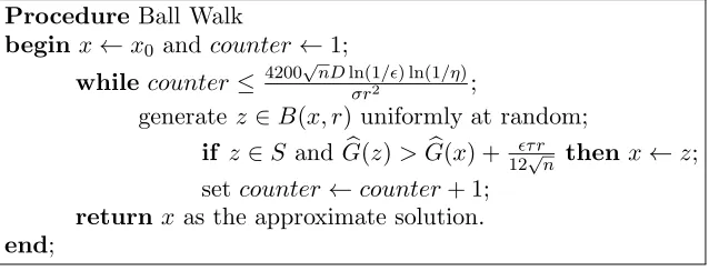
ProcedureBall Walk
beginx←x0 and counter←1;
while counter≤ 4200√nDln(1σr2/ǫ) ln(1/η);
generatez∈B(x, r) uniformly at random; if z∈S and G(z)>G(x) + 12ǫτ r√
n thenx←z;
[image:5.612.97.416.48.170.2]setcounter←counter+ 1; return x as the approximate solution. end;
Figure 1: The Ball Walk Algorithm
The Ball Walk algorithm aims at finding a pointxfor whichG(x)≥G(x∗)−ǫτ D with probability at least 1−η. The choices of the various parameters that we make now, may seem magic at this point of the text, but their justification will become clear later. Because of the uncertainty in the estimation of G, we must choose ǫ ≥ 24√nǫ0
τ r , so ǫ0 ≤ 24ǫτ r√n. The algorithm is described in Figure
1, where we choose r = min{r0,√Dn,90στ+3ǫτν√n}. Note that it might appear at first sight that assumption A.4 could be satisfied by simply choosing a large value of σ. However, the value ofr
must then be very small, and so the running time of the algorithm will be large.
The improvement we get in one step of Ball Walk will be examined below in Theorem 2.1. But first we give somepreliminary elementary estimates which will prove useful.
Lemma 2.1. Forn≥2, √n/3≤vol(Bn−1)/vol(Bn)≤2√n/3.
Proof. Since vol(Bn) =πn/2/Γ(n/2 + 1),
vol(Bn−1) vol(Bn)
= √ Γ(n/2 + 1)
π(Γ((n−1)/2 + 1).
Stirling’s approximation to the Gamma function values gives the conclusion after some calculation.
Lemma 2.2. For n ≥ 2, let U = {x = (x1, . . . , xn) ∈ B(0, r)|0 ≤ x1 ≤ cr/√n} be a slice of
B(0, r)⊂Rn, where 0< c <1. Then c/5≤vol(U)/vol(B(0, r))≤2c/3.
Proof. Since c≤1, elementary estimates give
c
√
n
1− 1
n
n−1 2 vol(B
n−1) vol(Bn) ≤
vol(U) vol(B) ≤
c
√
n
vol(Bn−1) vol(Bn)
.
Using Lemma 2.1 and (1−1/n)n−1 ≥e−1 now gives the conclusion.
Theorem 2.1. Let n≥3, and x ∈S be such that G(x) ≤G(x∗)−ǫτ D. With probability at least
σr/120 a point z is found in one step with
G(z) ≥ G(x) + ǫτ r 6√n,
Proof. First shrink B(x, r) to B(x, r′), with r′= (1−β)r, and β= 2
n. We writeB andB′ shortly
forB(x, r) and B(x, r′), respectively. Notice that
vol(B′) = (1−β)nvol(B).
Define g(x) = ∇∇GG((xx)), and v= xx∗∗−−xx. Consider the set
T1=B′∩S∩ {y|(y−x)Tg(x) ≥ − 5c1r′
√
n } ∩ {y|(y−x)
Tv≤ 5c2r′
√
n },
withc1 = 3σr′ and c2 = 12 −σr′. Note that the bound on r implies that c1 < ǫ/2≤ 12, and clearly
c2 < 12. Now T1 is obtained from B′ by cutting off the union of two caps and therefore, using Lemma 2.2,
vol(T1)≥vol(B′∩S)−( 1
2 −c2)vol(B ′)−(1
2 −c1)vol(B ′).
Thus, using assumption A.4 and the definition ofc1 and c2,
vol(T1) vol(B′) ≥
1 2 −σr
′−σr′−1 2+ 3σr
′ =σr′.
Letα= 3Dr√
n, and define the set
T2 ={αx∗+ (1−α)y|y∈T1}.
We claim thatT2is a subset ofB, each point of which gives the improvement stated in the theorem. Thus, its relative volume is a lower bound on the probability that such an improvement is attained in one step of the Ball Walk algorithm. This relative volume is in turn bounded as follows:
vol(T2) vol(B) ≥
(1−α)nvol(T1)
(1−β)−nvol(B′) ≥ (1−α)
n(1
−β)nσr′
= (1−α)n(1−β)n+1σr
≥ (8/9)3(1/3)4σr
≥ σr/120,
where the last but one inequality is implied by r≤ √D
n,n≥3, and the choices forα and β.
To show thatT2⊂B, we takez=αx∗+ (1−α)y for somey∈T1. and show that z−x ≤r.
z−x2 =α2x∗−x2+ (1−α)2y−x2+ 2α(1−α)(x∗−x)T(y−x). (1)
To bound the first term of the right-hand side of (1), we use the definition of α and the fact that
x∗−x ≤D, giving
α2x∗−x2 ≤
r
3D√n
2
D2 = r 2
9n. (2)
Sincey ∈B′ implies thaty−x ≤r′= (1−β)r and 0≤α, β≤1 implies that (1−α)2(1−β)2≤ (1−β), the second term of the right-hand side is bounded by
(1−α)2y−x2 ≤(1−β)r2 = (1− 2
n)r
Finally, the definitions of α,v,c2 andT1 imply
2α(1−α)(x∗−x)T(y−x)≤ 10
3 (1−β)c2
r2 n ≤
5r2
3n. (4)
(2), (3), (4) inserted in (1) yields
z−x2≤
1
9n+ 1−
2
n+
5 3n
r2 ≤r2.
Next we show thatz gives the desired improvement over x. By concavity of G
G(z)−G(x)≥α(G(x∗)−G(x)) + (1−α)(G(y)−G(x)). (5)
The second order Taylor expansion ofG iny aroundx yields
G(y)−G(x) = ∇G(x)T(y−x) + 1 2G
′′(w;x′)y−x2
≥ −5√c1r′
n ∇G(x) −
1 2νr
′2
≥ −5√c1r
n∇G(x) −
1 2νr
2
≥ −15σr
2
√
n ∇G(x) −
1 2νr
2, (6)
wherex′ ∈[x, y],w= (y−x)/y−x, and we used assumption A.3 for the first inequality. Using the definition of α, (5) and (6) yield
G(z)−G(x)≥ r
3D√n(G(x
∗)−G(x))−15√σ
n∇G(x)+
1 2ν
r2.
Since we assumedG(x∗)−G(x)≥ǫτ D, using ∇G(x) ≤τ (assumption A.2), leads to
G(z)−G(x)
G(x∗)−G(x) ≥
r
3D√n−
15στ /√n ǫτ D +
ν/2
ǫτ D
r2.
Since r≤ 90στ+3ǫτν√
n, a simple calculation now gives
G(z)−G(x)
G(x∗)−G(x) ≥
r
6D√n (7)
Hence
G(z)−G(x) ≥ r 6D√n
G(x∗)−G(x) ≥ ǫτ r 6√n,
as required. In this event,
G(z)−G(x) ≥ G(z)−G(x)−2ǫ0 ≥
ǫτ r
6√n− ǫτ r
12√n = ǫτ r
12√n,
If the Ball Walk accepts, then we know that
G(z)−G(x) ≥ G(z)−G(x)−2ǫ0 ≥
ǫτ r
12√n− ǫτ r
12√n = 0, (8)
thus the Ball Walk algorithm never causes the value ofG(x) to decrease.
Theorem 2.2. With probability at least 1−η, the number of samples from a ball that the Ball Walk algorithm requires to reach a point x with G(x∗)−G(x)≤ǫτ D is bounded from above by
4200√nDln(1/ǫ) ln(1/η)
σr2 .
Proof. From (7) in the proof of Theorem 2.1, with probability at least 120σr we have
G(x∗)−G(z)
G(x∗)−G(x) = 1−
G(z)−G(x)
G(x∗)−G(x) ≤ 1−
r
6D√n,
and the Ball Walk accepts the step. Moreover, the concavity ofGand assumption A.2 imply that
G(x∗)−G(y) ≤τ D for all feasibley, hence also for the starting point x0. Let us call a good step one in which the improvement is as in (7), and note that no step results in a decrease in G(x). Then, after kgood steps, we obtain a point xk with
G(x∗)−G(xk) ≤ 1− r 6D√n
k
τ D≤ τ Dexp− kr 6D√n
≤ ǫτ D.
when
k ≥ 6
√
nDlog(1/ǫ)
r .
Let K = 700kln(1/η)/(σr). Then, using Chernoff’s inequality, the probability that in K steps there are fewer thank good steps is at most
exp−1 3
5kln(1/η)−k
5kln(1/η)
2
5kln(1/η) = exp− k
5 ln(1/η)−12 15 ln(1/η)
≤ exp−kln(1/η) = ηk ≤ η,
providedη ≤e−1 and k≥1.
Note that the bound of Theorem 2.2 is indeed polynomial in the parameters of the problem, since
r is a rational function of the problem parameters.
3
Two-stage stochastic programming
In this section we describe briefly stochastic linear programming problems. Problems of this type have been studied since they were proposed in the mid 1950’s [2], [4], [30]. They model optimi-sation under uncertainty. Such models are useful in many practical situations. Obtaining exact information about all parameters in a practical optimisation problem is often impossible.
be exact information about the amounts needed to invest in a certain given project. At best one might hope to have some idea of what these parameter values could be, and to express this in the form of probability distributions. In this way we arrive at stochastic programming problems.
Suppose that we have a linear programming problem in which some parameters are random. The random variables we indicate by putting a tilde over them.
max px
subject to Ax≤b
˜
T x≤ξ˜
withb∈Rm, ˜ξ ∈Rd, and A anm×nmatrix, ˜T an d×n matrix, andp∈Rn.
We assume that probability distributions are given for the random matrix ˜T and the random vector ˜
ξ. The above model is clearly ill-defined since a solution x that is optimal for one realisation of ˜T
and ˜ξ may even be infeasible for another.
Two main directions have been taken in the literature to arrive at sensible models. In the con-ceptually easiest, violation of the uncertain constraints is allowed to occur with a probability that does not exceed a prespecified level, giving the so-calledprobabilistic constraints problem. The best comprehensive survey of this field is [25]. The paper of Kannan and Nolte [17] takes a similar approach to the probabilistic constraints problem that we take here for the model described next.
The other direction is the one we consider in this paper and is called the two-stage stochastic programming problem or the stochastic recourse problem. Conceptually one should think of the decision process taking place in two stages. In the first, values for the first stage variables x are chosen. In the second, upon a realisation of the random parameters, a recourse action is to be taken in case of infeasibilities. Costs are attached to the various possible recourse actions leading to the second stage (or recourse) problem, to choose the optimal action given the infeasibilities. The expected cost of the optimal recourse action is then added to the objective function. For a comprehensive review of the extensive literature we refer to [3], [11], [25].
A generic mathematical programming formulation for this problem is
max px+E[max{qy˜ |W y≤T x˜ −ξ, y˜ ∈Rn1 }]
subject to Ax≤b. (9)
with ˜q ∈Rn1 and W an d
×n1 matrix. In the literature W is sometimes allowed to be a random matrix. However, this may cause the feasible region to be non-convex in terms of x (see [31]). We concentrate on the so-called fixed recourse model in which W is fixed. Moreover, we assume that
W is such that for any x and any realisation of ˜T and ˜ξ there exists a feasible solution y in the second stage problem. This property of W is called the complete recourse property, and the model is accordingly called thecomplete recourse model(see e.g. [3]).
in Section 5. However, another serious obstruction against using Ball Walk is that this algorithm requires an oracle that gives function values on request. As will be clear from the next section, it is exactly the evaluation of the objective function which makes the two-stage stochastic programming problem so excessively hard to solve. Therefore, the assumption that a function evaluation oracle exists for these problems significantly hides their computational difficulty.
Therefore, before adapting the Ball Walk algorithm to solve two-stage stochastic programming problems in Section 5, we first devise a suitable function evaluation oracle in Section 4.
Our Ball Walk algorithm algorithm is certainly not among the first randomised approaches to solving two-stage stochastic programming problems. There is an extensive literature on sampling based methods, see a.o. [5, 13, 18, 20, 26]. In all these papers statistical convergence of the methods is analysed, but none considers complexity issues. The first one in that sense was the work by Kleiwegt, Shapiro and Honem-de-Mello, [19] in a version of the so-called sample average method, in which scenarios of the random parameters are sampled and then an approximate problem is solved, the so-called deterministic equivalent problem, with discrete distributions estimated by the samples. They give a bound on the number of samples needed to to find a near-optimal solution that is polynomial in the dimension of the problem. The running time is however also a function of a parameter based on the distribution of the scenarios. It was in [27] and the aforementioned papers of [29] and [23] that running times became independent of distribution functions.
4
Computation of the objective function
As we pointed out in the Introduction, the main difficulty in solving the two-stage stochastic programming problem is the computation of the objective function. We concentrate in the rest of the paper on the version of (9) in which only the right hand side coefficients ˜ξ are random. Thus,q
andT are fixed. We also suppress the tilde onξ. We use the notation Gfor the objective function, i.e.
max
x∈S G(x) =px+Q(x), (10)
with
Q(x) =Eξ[max{qy|W y≤T x−ξ, y∈Rn1}].
and
S ={x∈Rn|Ax≤b}
In this section we describe a fpras for evaluating Q(x) and therefore for evaluating the objective functionG(x). It is based on a Markov chain approach, where we sample approximately according to the known density function of ξ, compute the value of the linear program and take the average over the values obtained from the sample.
The only source of randomness is ξ, which we assume is described by a given density function
f :Rd→R. Thus,
Q(x) = v(T x−ξ)f(ξ)dξ
with
v(T x−ξ) = max{qy|W y≤T x−ξ, y∈Rn1 }.
We require some mild conditions onf. We cannot expect to approximateQefficiently for arbitrary
in the relative sense [14]. Therefore we assume the following conditions, borrowed from volume computation [1].
Assumptions B:
1. f is log-concave, i.e. logf is concave on its support suppf;
2. f has a negligible measure outsideB(0, R), i.e. for allϕ >0, there exists R≥4d such that ξ≥Rf(ξ)dξ≤ϕ;
3. logf is Lipschitz-continuous, i.e. there existsθ >0 such that|logf(ξ)−logf(ξ′)| ≤θξ−ξ′
for all ξ, ξ′ ∈suppf;
4. We are given a ξ0 ∈B(0, R) with f(ξ0)≥R−γd for some absolute constantγ, where R is as chosen in B.2 above. This implies that we know a good starting point for the Markov chain, a so called “warm start”;4
5. the directional derivative v′(w;T x−ξ) is uniformly bounded for all unit vectors w∈Rd, i.e. there exists λ >0 such that for all ξ∈suppf andx∈S,|v′(w;T x−ξ)| ≤λ;
6. The rows of T are scaled to have unit norm. Thus T ≤√d.
7. There exist x0 ∈ Rn, Rin, Rout ∈ R+ such that B(x0, Rin) ⊆ S ⊆ B(x0, Rout). Let κ =
Rout/Rin be therounding number or aspect ratio of the polytope S.
Conditions B.1–B.4 do not severely restrict the instances, since (with minor technical changes) all the most important distributions, for example those from the exponential family, meet the requirements.
Condition B.5 requires that the function v(·) does not vary too rapidly. Condition B.6 is clearly not restrictive, and B.7 is discussed in the next section. We don’t use either of B.6 or B.7 until the following section, but give them here to have a complete overview of all our conditions.
To sample according tof, we define a Metropolis random walk that hasf restricted toB(0, R) as its steady state density function. Note that, by assumption B.2, the restricted density ˆf satisfies
f ≤ fˆ≤ f /(1−ϕ). If ϕ is assumed negligible, then by B.1 and B.5 we can suppose that this simply contributes a negligible amount to the approximation error forQ(x). Thus we will not need to draw a distinction between f and ˆf in what follows and we will use the notation f, though it should read ˆf.
To sample fromf we define a random walk that hasf as its steady state density. One step of the random walk is defined as follows. Suppose the walk is at x ∈ B(0, R). We choose uniformly at random a pointyin a ball with centerxand radiusδ, to be specified later. Ifyis not inB(0, R), we stay at x. Otherwise, iff(y)≥f(x), we move to y, else we move to y with probability f(y)/f(x). Formally, the transition kernel p(x, y) (x =y) for moving fromx to y in one step of the random walk is given by
p(x, y) =
⎧ ⎨ ⎩
1
vol(B(0, δ))min
1,f(y) f(x)
if y∈B(0, R), 0<x−y ≤δ,
0 otherwise.
4
Note that p(x, x) is an atom 1−y=xp(x, y)dy. It is easy to see, by time reversibility, that the steady state distribution of this random walk has density proportional tof(x).
In the following we will use techniques and results from volume estimation [7, 16] to prove that this chain mixes rapidly, i.e. converges fast to the steady state. We first introduce some notation and state the relevant results from the literature.
Theorem 4.1. Dyer and Frieze [6]
Let S ⊂Rd be a convex body with diameter D andf be a log-concave function defined onS withπ
the induced probability measure on S. Let S1, S2 ⊂ S, t≤dist (S1, S2) = minx∈S1,y∈S2x−y. If
S0 =S \(S1∪S2)), then
min{π(S1), π(S2)} ≤
D
2tπ(S0). 2
The quantity 2/D is called the isoperimetric constant Iso(S) ofS.
Given a random walk with stationary distributionπ defined on a set S, its conductance is defined as
Φ = inf
{S⊂S|0<π(S)≤1/2}
SPu( ¯S)dπ(u)
π(S) ,
where Pu( ¯S) is the probability of moving in one step from point u inS ⊂ S to a point in ¯S, the
complement of S inS.
The local conductance of a Markov chain at a point x is defined as the probability of moving to any point y=x in one step.
Theorem 4.2. Kannan [15]
Consider a Metropolis random walk using balls of radius δ in a convex set S ⊂Rd which has local conductance at least χ at every point. Then the conductance Φ of the walk is at least
Iso(S)χ2δ
32√d . 2
Theorem 4.3. Lovasz and Simonovits [21]
Let f0 be the initial density of a Metropolis random walk on Rdwith stationary density f. Define
M(f0, f) = sup {S⊂Rd
|0<Sf≤1/2}
|Sf −
Sf0|
Sf
.
Let fk be the density of the Markov chain after k steps. Then
sup
S⊂Rd
Sf− Sfk
< M(f0, f)
1−Φ 2
2
k
. 2
Theorem 4.4. Using the Metropolis random walk, we can sample in B(0, R)⊂Rd according to a density f′ withsupS⊂Rd|
Sf−
Sf′|< ǫ in K′ steps, where
K′ = 8·104R2d3e4θ
ln1
ǫ + (γ+ 1)dlnR
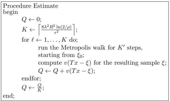
Procedure Estimate begin
Q←0;
K ←8λ2R2ǫln(22 /ρ)
;
forℓ←1, . . . , K do;
run the Metropolis walk forK′ steps, starting fromξ0;
computev(T x−ξ) for the resulting sampleξ;
Q←Q+v(T x−ξ); endfor;
[image:13.612.79.370.98.272.2]Q← KQ; end;
Figure 2: The approximation algorithm for Q(x)
Proof. Theorem 4.1 gives an isoperimetric constant of R1 for a random walk on B(0, R). The Lipschitz continuity (assumption B.3) implies that the acceptance function varies only by a factor e−θδ ≥ e−θδ over B(x, δ). Moreover, vol(B(x, δ)∩B(0, R)) ≥ 0.4B(x, δ), if x ∈ B(0, R). To see this note that the intersection contains a cap of B(x, δ) at distance at most δ2/(2R) from x, by elementary geometry. Lemma 2.2 with c = 1/(2R) now implies the volume of the cap is at least 1/2−1/(3R)>0.4, by assumption B.2. Thus, choosingδ= √1
dimplies a constant local conductance
χ≥ 0.4√e−θ
d .
Applying these results, Theorem 4.2 implies a lower bound on the conductance Φ of the walk of
1
200Rd√de2θ. Theorem 4.3 then yields
sup
S⊂Rd
Sf− Sf′
< M(f0, f)
1−Φ 2
2
K′
We choose the uniform distribution onB(ξ0, δ) as the initial densityf0, whereξ0 is the point guar-anteed by assumption B.4. assumption B.3 again implies that the acceptance function varies over
B(ξ0, δ) only by a factor θδ. These, together with assumption B.2, imply M(f0, f) = e−θR(γ+1)d, after some calculation.
# . . . .I admit that I could not reproduce the calculations, so I just replaced the θ bye−θ, supposing that our previous calculations were correct and using the
correct bound e−θδ ≥e−θδ . . . .#
In Figure 2 we define the procedureEstimatebased on the Markov chain described above to compute an approximation of the value of Q(x).
this at various places. Maybe you see a better way to use the new Assumption B.5
#
Theorem 4.5. With probability 1−ρ, procedure Estimate computes QK(x)∈[Q(x)−ǫ, Q(x) +ǫ] in K =8L2ln(2ǫ2 /ρ)
samples.
Proof. Let QK(x) = K1 Ki=1v(T x−ξi), with ξ1,· · · , ξK independent samples generated by the
Metropolis random walk. Thus,E[QK(x)] = v(T x−ξ)fK′(ξ)dξ, wherefK′ is the density produced
by the Metropolis random walk when run with error parameter ǫ′ = ǫ/4λ. Since we assume that the directional derivative ofvis uniformly bounded byλby assumption B.5, Hoeffding’s inequality implies
Pr{|QK(x)−E[QK(x)]|> 12ǫ} ≤2 exp
− ǫ
2K2 8(λR)2
,
# . . . .Check Hoeffding’s. Should be K2 i.o. K if I am right. This would have
implications for the choice of K . . . #
sinceK ≥8λ2R2ln(2/ρ)ǫ−2. Theorem 4.4 yields
|E[QK(x)]−Q(x)| =
v(T x−ξ)fK′(ξ)dξ− v(T x−ξ)f(ξ)dξ
≤ λR |f(ξ)−fK′(ξ)|dξ
= 2λR
f≤fK′
(fK′(ξ)−f(ξ))dξ
≤ 2λRǫ′ = 12ǫ,
Combining these, we see that Pr{|QK(x)−Q(x)|> ǫ} ≤ρ.
Corollary 4.1. In K·K′ = OγR4dǫ32λ2e4θ log1ǫ logRlog1ρ
steps, procedure Estimate computes
QK(x)∈[Q(x)−ǫ, Q(x) +ǫ]. 2
Using the approximation algorithm for the objective functionGand applying the ellipsoid algorithm in [12] to our problem, under our assumptions we would have a fpras for the stochastic recourse problem. The following theorem follows easily from taking ρ =ζ/N in Theorem 4.5, where N is the required number of steps of the ellipsoid algorithm.
Theorem 4.6. Under assumptions B.1–B.5, with probability at least 1−ζ, the ellipsoid algo-rithm, using procedure Estimate to approximately evaluate G, will solve the two-stage stochastic programming problem (10) to within additive errorǫ, in a number of arithmetic operations bounded polynomially in the input parameters, 1/ǫ and log 1/ζ. 2
5
Random directions for two-stage stochastic programming
In this section we will extend the Ball Walk approach to solve the two stage stochastic programming problem. Recall the formulation (10) in Section 4. We assume conditions B.1–B.5, which we required previously for the randomized approximate computation ofQ(x), and now we also assume that condition B.6 is satisfied.
It turns out that these conditions on the density function also imply smoothness of the objective function, required for the Ball Walk algorithm of Section 2, as we will show.
Lemma 5.1. Suppose x∈S. Under assumptions B.1–B.6, we have
∇G(x) ≤ p+λ√d, and ∇2G(x) ≤λθd.
As a result we may choose the smoothness parameters τ and ν of G (assumptions A.2, A.3) to be p+λ√dand λθd, respectively.
Proof. Let wbe a unit vector and u=T w/T w. Then
|Q′(w;x)| =
tlim→0
v(T x+tT w−ξ)f(ξ)−v(T x−ξ)f(ξ)
t dξ = tlim→0
v(T x+tT w−ξ)−v(T x−ξ)
t f(ξ)dξ
= T w
v′(u;T x−ξ)f(ξ)dξ
≤ T w |v′(u;T x−ξ)|f(ξ)dξ
≤ λT w f(ξ)dξ
≤ λ√d,
where we have used B.6 to give T w ≤√d. Also
|Q′′(w;x)| = T w
limt→0
v′(u;T x+tT w−ξ)f(ξ)−v′(u;T x−ξ)f(ξ)
t dξ
= T w
limt→0
v′(u;T x−ξ)f(ξ+tT w)−v′(u;T x−ξ)f(ξ)
t dξ
= T w2
v′(u;T x−ξ)f′(u;ξ)dξ
≤ T w2 |v′(u;T x−ξ)| · |f′(u;ξ)|dξ
≤ θT w2 |v′(u;T x−ξ)|f(ξ)dξ
≤ λθT w2 f(ξ)dξ
≤ λθd,
Thus, assumptions A.2 and A.3 in Section 2 are satisfied. We know that G is concave, satisfying also assumption A.1. Therefore, we need to be concerned now with smoothing the underlying feasible setS ={x∈Rn|Ax≤b}. SinceS is a polyhedron, it is not smooth. Therefore we use the “roundedness” assumption B.7 on S. This allows us to consider a slightly larger (non-polyhedral) set, which is indeed smooth, and apply the Ball Walk to this larger set.
Recall κ =Rout/Rin. Note that κ resembles a “condition number”: it is small if the polytope is “well-rounded” and large if it is not. Thus we will assumeκ is not too large. In fact any polytope can be “rounded” to have κ = O(√n), but here this may be undesirable since it can adversely affect the parameters of G. From now on we assume that S satisfies the above assumption.
To facilitate the exposition, let A(i) denote theith row ofA, and supposeA is normalised so that
A(i)= 1 (i= 1, . . . , m). Then, forx∈Rn, let
(A(i)x−bi)+=
A(i)x−bi if A(i)x > bi,
0 otherwise,
be the distance from x to the halfspace A(i)y ≤ bi. Consider the function F(x) =mi=1((A(i)x−
bi)+)2, and, for a given μ >0, define the setSµ={x ∈Rn|F(x)≤μ}. Note that S ⊆Sµ and Sµ
is convex. The following lemmas establish the required smoothness condition forSµ.
Lemma 5.2. For all x, z∈Rn,z= 1, 0≤F′′(z;x)≤2m.
Proof. We have
∇F(x) = 2
i∈I(x)
(A(i)x−bi)A(i), (11)
whereI(x) ={i:A(i)x > b
i}. SinceF′(z;x) =∇F(x).z,
F′′(z;x) = 2
i∈I(x)
(A(i)z)2. (12)
Clearly F′′(z;x) ≥ 0, and the upper bound follows from |I(x)| ≤ m and the Cauchy-Schwarz inequality.
In particular, it follows thatF is a convex function.
Lemma 5.3. Let S have rounding number κ and 0< μ≤1. Then, for all x∈Sµ,
κ∇F(x) ≥F(x).
Proof. Assume without loss that x0 = 0 and Rin = 1, soRout =κ. Also bi ≥1 (i= 1, . . . , m), by
considering the points A(i) ∈∂B(0,1). Fix x∈S
µ, let
ψ= min 1≤i≤m
xbi
A(i)x :A
(i)x >0,
and let ℓ be the minimizing i. Let ˜x = ψx/x, so ψ = x˜. Clearly ψ ≤ κ, since otherwise
A(i)x˜≤bi (i= 1, . . . , m), but ˜x /∈B(0, κ). Now √μ
Thusx ≤(1 +√μ)x˜ ≤2κ. Thus, from (11),
∇F(x).x= 2
i∈I(x)
(A(i)x−bi)A(i)x≥2
i∈I(x)
(A(i)x−bi)≥2
F(x),
sinceA(i)x > bi ≥1 fori∈I(x) andF(x) =i∈I(x)(A(i)x−bi)2. Therefore, using Cauchy-Schwarz,
∇F(x) ≥2F(x)/x ≥F(x)/κ,
and the result follows.
Lemma 5.4. Let 0< μ≤1, and σ = (2mκ/3)n/μ. Then, for all x∈Sµ,
vol(B(x, r)∩Sµ)/vol(B(x, r))≥ 12−σr.
Proof. Assume without loss thatxis on the boundary ofSµ. Using Taylor’s theorem and Lemma 5.2,
for any displacement z,
F(x+z)≤F(x) +∇F(x).z+mz2=μ+∇F(x).z+mz2,
and the subgradient inequality gives
F(x+z)≥F(x) +∇F(x).z=μ+∇F(x).z.
Thus, ifF(x+z) =μ,−mz2≤ ∇F(x).z ≤0. Let H denote the half-space∇F(x).z ≤0, and ∂H
its boundary. Then, using Lemma 5.3,
dist (z, ∂H) = −∇F(x).z
∇F(x) ≤
mz2
∇F(x) ≤
mκz2
F(x) =
mκz2
√μ .
Letting B denote B(x, r), we see that B∩Sµ contains a cap of B at distance at most mκr2/√μ
from x. Thus, by Lemma 2.2,
vol(B∩Sµ)
vol(B) ≥ 1 2−
2mκ√n
3√μ r.
Using the last two lemmas we can now apply the Ball Walk to optimize G over Sµ. But, we are
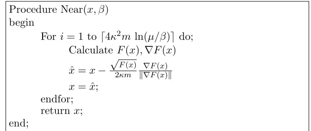
of course interested in optimizing G over the set S ⊂ Sµ. Thus, we will use Procedure Near (see
Figure 5), which finds a point arbitrarily close to S after we have optimized over the larger set
Sµ. The idea is to go repeatedly along the gradient of F, which is easy to compute, until we are
exponentially close to S. We will show that this procedure yields a point that is not much worse than the point resulting from the Ball Walk Algorithm, for an appropriate choice ofμ.
Theorem 5.1. Let x ∈ Sµ. Then, for any β < μ, procedure Near finds a y ∈ Sβ such that x−y ≤2μ/βln(μ/β). The running time isO(κ2m2nln(μ/β)).
Proof. The claim on the running time is easy to verify. Without loss, we will prove the lemma for a pointx on the boundary ofSµ, i.e. F(x) =μ. We start the procedure atx withF(x) =μand
ˆ
x=x−
F(x) 2κm
∇F(x)
Procedure Near(x, β) begin
Fori= 1 to ⌈4κ2m ln(μ/β)⌉ do; CalculateF(x),∇F(x)
ˆ
x=x−
√ F(x) 2κm ∇
F(x) ∇F(x)
[image:18.612.75.389.138.271.2]x= ˆx; endfor; returnx; end;
Figure 3: The Procedure Near
Using Lemma 5.2, the Taylor expansion yields
F(ˆx)≤F(x)−
F(x)
2κm ∇F(x)+m
F(x) 2κm
2
.
Now, using Lemma 5.3, this implies
F(ˆx)≤F(x)−(
F(x))2 2κ2m +
F(x)
4κ2m =F(x)
1− 1
4κ2m
.
We repeat this process k= 4κ2mlog(μ/β) times to get a pointy with
F(y)≤F(x)
1− 1 4κ2m
k ≤μ
1− 1 4κ2m
k ≤β.
Furthermore, lettingy be the final point returned by Near,
y−x ≤k
√μ
2κm ≤2κ
√μln(μ/β).
Hence, using the subgradient inequality,
G(y)≥G(x)−τy−x ≥G(x)−2τ κ√μln(μ/β).
Thus, sinceμ≤1, we will have G(y)≥G(x)−ǫprovided
μ≤
ǫ
2τ κln(1/β)
2
. (13)
Note that this is polynomial in the relevant parameters, in particular the number of bits of accuracy required.
Theorem 5.2. Under the assumptions B.1–B.7, with probability at least (1−ζ), an application of the Ball Walk combined with the procedures Estimateand Near will find y with
G(y)≥G(x∗)−ǫ
and
Ay≤b+β,
in time polynomial in the parameters of the problem, 1/ǫ, log(1/β) and log(1/ζ).
Proof. By using a small enough error probability at each step, the probability of making an error can be made at mostζover any polynomial number of steps (cf. the discussion before Theorem 4.6).
Chooseμ=2τ κln(1ǫ /β)2. Lemmas 5.1, 5.4 and Theorems 4.5, 5.1 then imply the theorem.
6
Postlude
We have described a simple randomized approximation scheme for convex optimisation problems, with two-stage stochastic programming problems as the main application.
There have been several proposals to use random walks for convex optimisation since this paper was first written. The algorithm of Bertsimas and Vempala [?] uses random walks to generate hyperplanes which “bisect” the solution space. Repeating this sufficiently many times locates the solution to any desired precision. This is a very different approach from the algorithm given here. The computational complexity of Bertsimas and Vempala’s algorithm is polynomial in terms of a standard measure of the size of the input, whereas we have worked with a different, less standard, measure of input size.
In [?], Lov´asz and Vempala adapt their “hit-and-run” algorithm for sampling from convex sets to optimise a logconcave function. The algorithm proceeds in phases, by modifying the objective function and sampling from the associated logconcave distribution, until an almost-optimal point is identified. The algorithm is shown to have polynomial time complexity in the standard model.
The paper of Kannan and Narayanan [?] uses random walks, similarly to the way they are used here, to optimize over polytopes. However, their steps are adaptive - they depend on the shape of the “Dikin ellipsoid” at the current point. These ellipsoids depend on knowing all the linear constraints and so the method only works for polytopes. It is an open question whether such an adaptive method exists for general convex sets, and hence to improve the algorithm presented here.
With respect to the application, it was as early as 1968 that Ermoliev and Shor proposed a random walk, based on stochastic gradients, to solve the two-stage stochastic programming model and ana-lyzed global convergence [10]. As for the analysis of randomised algorithms for two-stage stochastic programming problems from a complexity theoretic point of view, some other papers close to our approach have appeared in the literature more recently [27, 29, 23]. We compare our paper to the ones by Shmoys and Swamy [29] and by Nesterov and Vial [23]. We refer to [23] for a comparison to the results on the sample average method by Shapiro and Nemirovski [27].
Shmoys and Swamy [28]) that confirmed that the community became ready to accept these new notions.”
Both [29] and [23] use stochastic subgradients. In [23] this is employed in a subgradient-descent approach for optimization of the convex objective function, whereas in [29] it is employed in an ellipsoid method. In this way expensive function evaluations can be avoided to find the near-optimal solution. Indeed in [29] the optimal solution value does not belong to the output of their method. In [23] only in the final solution the function evaluation is made, by sampling from the distribution of the stochastic parameters. Of course, this could be done as well in [29] but it would reduce the strength of their complexity result (that we discuss below), which in fact it does also in [23]. We use the simple Ball Walk algorithm, which is more stable than the ellipsoid algorithm, and outputs both solution and its value. At this stage of their development all three algorithms are only of academic interest.
A limitation of [29] is that their result applies only to problems in which the first and the second stage decisions are of exactly the same quality. The second stage cost coefficients are higher than the first stage ones. The algorithm of [23] and our algorithm apply to any setting, including hierarchical planning models, where the first stage concerns a longer term strategic decision and the second stage short term operational decisions.
All three approaches yield an fpras under more or less severe assumptions. The advantage of the limitation in [29] is that it allows a very elegant complexity result: it suffices to assume that a bound on the maximum ratio between the second and first stage cost coefficients is given as a fixed parameter; the running time of their algorithm is polynomial in this parameter. They even show that essentially this cannot be improved. In our case the fixed parameter is the uniform bound on directional derivatives of the value function. Similarly, in [23] a uniform bound on the Euclidean norm of the stochastic subgradients is the fixed parameter if, as in [29], only the solution is output. In order to compute also the value of the solution the running time of the algorithm becomes also a polynomial function of a bound on the variation of the objective value over its feasible domain and over the probability space of the stochastic parameters.
All three approaches give an fpras (under the various above restrictions) under the “black box model” as it was called in [29]. Under this model the size of the input needed to describe the probability distributions of the random problem parameters is not taken into account in the running time. In [29] and in [23] an oracle is assumed to give realisations of the random parameters. We specify how to sample form the distributions. To avoid computational problems we restrict to specific classes of probability distributions.
As it holds for the other methods, it remains to be seen whether the method that we propose here is a practically efficient method for solving two-stage stochastic programming problems. In any case it may provide a starting point for a more practical method. For example, it is likely that function evaluations do not have to be so precise if we are still far away from the optimum. Indeed, stochastic programmers have proposed methods that work with more and more accurate function evaluations as their methods proceed. It remains a challenge to incorporate these and other ideas that have been developed in stochastic programming research into our algorithmic framework.
References
[1] Applegate, D., Kannan, R. Sampling and integration of near log-concave functions.Proceedings of the 23th ACM Symposium on the Theory of Computing, 1990, pp. 156–163,
[2] Beale, E.M. On minimizing a convex function subject to linear inequalities. Journal of the Royal Statistical Society 17, 1955, pp. 173–184.
[3] Birge J., Louveaux F. Introduction to stochastic programming, Springer-Verlag, New York, 1997.
[4] Dantzig, G. Linear Programming under uncertainty. Management Science 1, 1955, pp. 197– 206.
[5] Dupaˇcov`a, J., Wets, R.J.-B. Asymptotic behavior of statistical estimators and of optimal solutions of stochastic optimization problems.Annals of Statistics 16, 1988, pp 1517-1549.
[6] Dyer, M. and Frieze, A. Computing the volume of convex bodies: a case where randomness provably helps. Probabilistic Combinatorics and its Applications, Proceedings of AMS Sym-posia in Applied Mathematics Vol. 44, 1991, pp. 123-169.
[7] Dyer, M., Frieze, A., Kannan, R. A random polynomial time algorithm for approximating the volume of convex bodies.Journal of the ACM 38, 1991, pp. 1–17.
[8] Dyer, M., Kannan, R., Stougie, L. A simple algorithm randomised algorithm for convex optimis; Application to two-stage stochastic programming. Technical Report SPOR-Report 2002-05, Department of Mathematics and Computer Science, Eindhoven Tecnical Universtiy, Eindhoven, 2002.
[9] Dyer, M., Stougie, L. A note on the complexity of some stochastic optimization problems,
Mathematical Programming 106, 2006, pp. 423–432.
[10] Ermoliev, Y., Shor, N.Z. Method of random walk for the two-stage problem of stochastic programming and its generalization.Kibernetica 4, 1968, pp. 59–60.
[11] Ermoliev, Y., Wets, R.J-B, (eds.) Numerical techniques for stochastic optimization, Springer-Verlag, Berlin, 1988.
[12] Gr¨otschel, M., Lovasz, L., Schrijver, A.Geometric algorithms and combinatorial optimization. Springer Verlag, New York, 1988.
[13] Higle, J.L., Sen, S. Stochastic decomposition: An algorithm for two stage linear programs with recourse.Mathematics of Operations Research 16, 1991, pp 650-699.
[14] Jerrum, M., Sinclair, A. The Markov chain Monte Carlo method: an approach to approximate counting and integration. InApproximation algorithms for NP-hard problems, D. S. Hochbaum (ed.), PWS Publishing, Boston, 1996, pp. 482–520.
[15] Kannan, R. Markov chains and polynomial time algorithms.Proceedings of the 35th Symposium on Foundations of Computer Science, 1994, pp. 656–671.
[17] Kannan, R., Nolte, A. Local search in smooth convex sets.Proceedings of the 39th Symposium on Foundations of Computer Science, 1998, pp. 218–226.
[18] King, A.J., Rockafellar, R.T. Asymptotic theory for solutions in statistical estimation and stochastic optimization.Mathematics of Operations Research 18, 1993, pp 148-162.
[19] Kleywegt, A.J., Shapiro, A., Homem-De-Mello, T. The sample average approximation method for stochastic discrete optimization.SIAM Journal of Optimization 12, 2001, pp. 479–502.
[20] Mak, W.-K., Morton, D.P., Wood, R.K. Monte-Carlo bounding techniques for determining solution quality in stochastic programs.Operations Research Letters 24, 1999, pp 47-56.
[21] Lovasz, L., Simonovits, M. Random walks in a convex body and an improved volume algorithm.
Random Structures and Algorithms 4, 1993, pp. 359–412.
[22] Nemirovski, A., Nesterov, Y.Interior point polynomial methods in convex programming, SIAM Press, 1994.
[23] Nesterov, Y., Vial, J-P. Confidence level solutions for stochastic programming.Automatica 6, 2008, pp. 1559–1568.
[24] Nesterov, Y., Vial, J-P. Confidence level solutions for stochastic programming, Technical Re-port Core Discussion Papers, 2000. http://www.core.ucl.ac.be/services/psfiles/dp00/dp2000-13.pdf
[25] Prekopa, A., Stochastic programming, Mathematics and its applications Vol. 324, Kluwer, Dordrecht, 1995.
[26] Shapiro, A., Homem-de-Mello, T. A simulation-based approach to two-stage stochastic pro-gramming with recourse. Mathematical Programming 81, 1998, pp 301-325.
[27] On complexity of stochastic programming problems. In Jeyakumar, V., Rubinov, A.M. (eds.)
Continuous optimization: Current trends and applications, Springer Verlag, Berlin, 2005, pp 111–144.
[28] Shmoys, D.B., Swamy, C. Stochastic optimization is (almost) as easy as deterministic opti-mization. In Proceedings of the 45th Annual IEEE Symposium on Foundations of Computer Science,2004, pp. 228237.
[29] Shmoys, D.B., Swamy, C. An approximation scheme for stochastic linear programming and its applications to stochastic integer programs.Journal of the ACM 53, 2006, pp. 978–1012.
[30] Tintner, G. Stochastic linear programming with applications to agricultural economics. In Antosiewicz, H.A. (ed.)Proceedings of the Second Symposium on Linear Programming, Wash-ington, 1955, pp. 197–207.
[31] Wets, R. Stochastic programming: solution techniques and approximation. In Bachem, A., Groetschel M., Korte, B. (eds.)Mathematical programming: the state of the art (Bonn, 1982), Springer, Berlin, 1983, pp. 566–603.