Adaptive Greedy Algorithm With Application to Nonlinear Communications

Adaptive Greedy Algorithm With

Application to Nonlinear Communications

The Harvard community has made this

article openly available.

Please share

how

this access benefits you. Your story matters

Citation

Mileounis, Garasimos, Behtash Babadi, Nicholas Kalouptsidis, and

Vahid Tarokh. 2010. IEEE Transactions on Signal Processing 58(6):

5424024.

Published Version

http://ieeexplore.ieee.org/xpl/freeabs_all.jsp?arnumber=5424024

Citable link

http://nrs.harvard.edu/urn-3:HUL.InstRepos:4687242

An adaptive greedy algorithm with application to

nonlinear communications

Gerasimos Mileounis,

Student Member, IEEE,

Behtash Babadi,

Nicholas Kalouptsidis, and Vahid Tarokh,

Fellow, IEEE,

Abstract—Greedy algorithms form an essential tool for com-pressed sensing. However, their inherent batch mode discour-ages their use in time-varying environments due to significant complexity and storage requirements. In this paper a powerful greedy scheme developed in [1], [2], is converted into an adaptive algorithm which is applied to estimation of a class of nonlinear communication systems. Performance is assessed via computer simulations on a variety of linear and nonlinear channels; all confirm significant improvements over conventional methods.

Index Terms—Adaptive filters, ARMA processes, Nonlinear systems, Equalizers, Compressed Sensing.

I. INTRODUCTION

Many real-life systems admit sparse representations, that is they are characterized by small number of non-zero coeffi-cients. Sparse systems can be found in many signal processing [3] and communications applications [4]–[6]. For instance, in High Definition Television the significant echoes form a cluster, yet interarrival times between different clusters can be very long [4]. In wireless multipath channels there is a relatively small number of clusters of significant paths [5]. Finally, underwater acoustic channels exhibit long time delays between the multipath terms due to reflections off the sea surface or sea floor [6].

Two major algorithmic approaches to compressive sensing are `1-minimization (basis pursuit) and greedy algorithms

(matching pursuit). Basis pursuit methods solve a convex minimization problem, which replaces the `0 quasi-norm by

the`1norm. The convex minimization problem can be solved

using linear programming methods, and is thus executed in polynomial time [7]. Greedy algorithms, on the other hand, iteratively compute the support set of the signal and construct an approximation to it, until a halting condition is met [1], [2], [8]–[11]. Both of the above approaches pose their own ad-vantages and disadad-vantages.`1-minimization methods provide

theoretical performance guarantees, but they lack the speed of greedy techniques. Recently developed greedy algorithms, such as those developed in [1], [2], [10], deliver some of the same guarantee as `1-minimization approaches with less

computational cost and storage.

Copyright (c) 2010 IEEE. Personal use of this material is permitted. However, permission to use this material for any other purposes must be obtained from the IEEE by sending a request to [email protected]. G. Mileounis and N. Kalouptsidis are with the Department of Informatics and Telecommunications, Division of Communications and Signal Processing, University of Athens, Greece (email:{gmil,kalou}@di.uoa.gr).

B. Babadi and V. Tarokh are with the School of Engineering and Ap-plied Sciences, Harvard University, Cambridge, MA02138 USA (e-mail: {behtash,vahid}@seas. harvard.edu).

Many signal processing applications [4]–[6] require adap-tive estimation with minimal complexity and small memory re-quirements. Existing approaches to sparse adaptive estimation use the`1-minimization technique, in order to improve the

per-formance of conventional algorithms. Chen et al. [12] incorpo-rated two different sparsity constraints (the`1and the log-sum

penalty functions) into the quadratic cost of the standard Least Mean Squares (LMS) to improve the filtering performance on sparse systems. In [13], Angelosante et al. developed a recursive subgradient-based approach for solving the batch Lasso estimator. An`1-regularized RLS type algorithm based

on a low complexity Expectation-Maximization is derived in [14] by Babadi et al. Sparse adaptive`1-regularized algorithms

based on Kalman filtering and Expectation Maximization are reported in [15] by Kalouptsidis et al.

In contrast to the above work on adaptive sparse identifi-cation, this paper focuses on the greedy viewpoint. Greedy algorithms in their ordinary mode of operation, have an inherent batch mode, and hence are not suitable for time-varying environments. This paper establishes a conversion pro-cedure that turns greedy algorithms into adaptive schemes for sparse system identification. In particular, a Sparse Adaptive Orthogonal Matching Pursuit (SpAdOMP) algorithm of linear complexity is developed, based on existing greedy algorithms [1], [2], that provide optimal performance guarantees. Also, the steady-state Mean Square Error (MSE) of the SpAdOMP algorithm is studied analytically. The developed algorithm is used to estimate ARMA and Nonlinear ARMA channels. It is shown that channel inversion for these channels, maintains sparsity and that it is equivalent to channel estimation. Com-puter simulations reveal that the proposed algorithm outper-forms most existing adaptive algorithms for sparse channel estimation.

The paper is structured as follows. The problem formulation and literature review are addressed in section II. Section III describes the established algorithm, the steady-state error anal-ysis and applications to nonlinear communication channels. Computer simulations are presented in section IV. Conclusions and future work are discussed in section V.

II. GREEDY METHODS AND THECOSAMPALGORITHM

Consider the noisy representation of a vector y(n) = [y1,· · ·, yn]T in terms of a basis arranged in the columns of

a matrixΦ(n)at timen

2 IEEE TRANSACTIONS ON SIGNAL PROCESSING, VOL. XX, NO. XX, MONTH 2010

where c is the parameter vector, Φ(n) = [φ(1), . . . ,φ(n)]T

andη(n) = [η1, . . . , ηn]T is the additive noise. The

measure-ment matrix Φ(n)∈Cn×N _{is often referred to as dictionary}

and the parameter vector c is assumed to be sparse, i.e.,

kck`0 ¿ N, where k · k`0 =|supp(·)| is the `0 quasi-norm.

We will call the parameter vectors-sparse when it contains at most snon-zero entries.

Recovery of the unknown parameter vectorccan be pursued by finding the sparsest estimate of c which satisfies the `2

norm error toleranceδ

min

c kck`0 subject to ky(n)−Φ(n)ck`2 ≤δ. (P`0)

Convex relaxation methods cope with the intractability of the above formulation by approximating the`0 quasi-norm by the

convex `1 norm. The set of resulting techniques is referred

to as `1-minimization. The `2 constraint can be interpreted

as a noise removal mechanism when δ ≥ kη(n)k`2. The

`1-minimization approach is a convex optimization problem

and can be solved by linear programming methods [7], [16], projected gradient methods [17] and iterative thresholding [18].

The exact conditions for retrieving the sparse vector rely either on the coherence of the measurement matrix [19] or on the Restricted Isometry Property (RIP) [16]. A measurement matrix Φ(n) satisfies the Restricted Isometry Property for δs(n)∈(0,1) if we have

¡

1−δs(n)

¢

kck2`2 ≤ kΦ(n)ck

2

`2 ≤ ¡

1 +δs(n)

¢

kck2`2 (2)

for alls-sparsec. Whenδs(n)is small, the restricted isometry

property implies that the set of columns of Φ(n) approxi-mately form an orthonormal system.

A. The CoSaMP greedy algorithm

Greedy algorithms provide an alternative approach to `1

-minimization. For the recovery of a sparse signal in the presence of noise, greedy algorithms iteratively improve the current estimate for the parameter vectorcby modifying one or more parameters until a halting condition is met. The basic principle behind greedy algorithms is to iteratively find the support set of the sparse vector and reconstruct the signal using the restricted support Least Squares (LS) estimate. The computational complexity of these algorithms depends on the number of iterations required to find the correct support set. One of the earliest algorithms proposed for sparse signal recovery is the Orthogonal Matching Pursuit (OMP) [8], [9], [19]. At each iteration, OMP finds the column of Φ(n)most correlated with the residual, v(n) =y(n)−Φ(n)ˆc, using the proxy signalp(n) =Φ∗T(n)v(n)(whereA∗T(n)denotes the conjugate transpose of the matrixA(n)∈Cn×N_{), and adds it}

to the support set. Then, it solves the following least squares problem:

ˆ

c= arg min

z ky(n)−Φ(n)zk`2

and finally updates the residual by removing the contribution of the latter column. By repeating this procedure a total of s times, the support set ofcis recovered. Although OMP is quite fast, it is unknown whether it succeeds on noisy measurements.

An alternative algorithm, called Stagewise OMP (StOMP), was proposed in [11]. Unlike OMP, it selects all components of the proxy signal whose values are above a certain threshold. Due to the multiple selection step, StOMP achieves better runtime than OMP. Parameter tuning in StOMP might be difficult and there are rigorous asymptotic results available.

A more sophisticated algorithm has been recently developed by Needell and Vershynin, and it is known as Regularized OMP (ROMP) [10]. ROMP chooses theslargest components of the proxy signal, followed by a regularization step, to ensure that not too many incorrect components are selected. For a measurement matrix Φ(n) with RIP constant δ2s =

0.03/√logs, ROMP provides uniform and stable recovery results. The recovery bounds obtained in [10] are optimal up to a logarithmic factor. Tighter recovery bounds which avoid the presence of the logarithmic factor are obtained by Needell and Tropp via the Compressed Sampling Matching Pursuit algorithm (CoSaMP) [1]. CoSaMP provides tighter recovery bounds than ROMP optimal up to a constant factor (which is a function of the RIP constants). An algorithm similar to the CoSaMP, was presented by Dai and Milenkovic and is known as Subspace Pursuit (SP) [2].

As with most greedy algorithms, CoSaMP takes advantage of the measurement matrix Φ(n) which is approximately orthonormal (Φ∗T(n)Φ(n)is close to the identity). Hence, the largest components of the signal proxyp(n) =Φ∗T(n)Φ(n)c

is most likely to correspond to the non-zero entries ofc. Next, the algorithm adds the largest components of the signal proxy to the running support set and performs least squares to get an estimate for the signal. Finally, it prunes the least square estimation and updates the error residual. The main ingredients of the CoSaMP algorithm are outlined below:

1) Identificationof the largest2scomponents of the proxy signal

2) Support Merger, which forms the union of the set of newly identified components with the set of indices corresponding to the s largest components of the least square estimate obtained in the previous iteration 3) Estimationvia least squares on the merged set of

com-ponents

4) Pruning, which restricts the LS estimate to its slargest components

5) Sample update, which updates the error residual. The above steps are repeated until a halting criterion is met. The main difference between CoSaMP and SP is in the identification step where the SP algorithm chooses theslargest components.

TABLE I SPADOMP ALGORITHM

Algorithm description Complexity

c(0) = 0,w(0) = 0,p(0) = 0 {Initiliazation}

v(0) =y(0) {Initial residual}

0< λ≤1 {Forgetting factor}

0< µ <2λ−1

max {Step size}

For n:= 1,2, . . .do

1: p(n) =λp(n−1) +φ∗_{(n−1)v(n−1) {Form signal proxy} N}

2: Ω = supp(p2s(n)) {Identify large components} N

3: Λ = Ω∪supp(c(n−1)) {Merge supports} s 4: ε(n) =y(n)−φT

|Λ(n)w|Λ(n−1) {Prediction error} s

5: w|Λ(n) =w|Λ(n−1) +µφ∗|Λ(n)ε(n) {LMS iteration} s

6: Λs= max(|w|Λ(n)|, s) {Obtain the pruned support} s

7: c|Λs(n) =w|Λs(n), c|Λcs(n) =0 {Prune the LMS estimates}

8: v(n) =y(n)−φT_{(n)c(n) {Update error residual} s}

end For O(N)

analysis on CoSaMP/SP due to their superior performance, but similar ideas are applicable to other greedy algorithms as well.

III. SPARSEADAPTIVEORTHOGONALMATCHING PURSUITALGORITHM

This section starts by converting CoSaMP and SP algo-rithms [1], [2] into an adaptive scheme. The derived algorithm is then used to estimate sparse Nonlinear ARMA channels.

The proposed algorithm relies on three modifications to the CoSaMP/SP structure: the proxy identification, estimation and error residual update. The error residual is now evaluated by

v(n) =y(n)−φT(n)c(n). (3) The above formula involves the current sample only, in contrast to the CoSaMP/SP scheme which requires all the previous samples. Eq. (3) requires scomplex multiplications, whereas the cost of the sample update in the CoSaMP/SP is sn multiplications. A new proxy signal that is more suitable for the adaptive mode, can be defined as:

p(n) =

n−1

X

i=1

λn−1−i_φ∗_(i)v(i)

and is updated by

p(n) =λp(n−1) +φ∗(n−1)v(n−1)

where the forgetting factorλ∈(0,1]is incorporated in order to give less weight in the past and more weight to recent data. This way the derived algorithm is capable of capturing variations on the support set of the parameter vectorc. In the case of a time-invariant environment,λshould be set to1. The addition of the forgetting factor mechanism requires redefining the Restricted Isometry Property as follows:

Definition 1. A measurement matrix Φ(n) satisfies the Exponentially-weighted Restricted Isometry Property (ERIP) for λ∈(0,1]and δs(λ, n)∈(0,1), if we have

¡

1−δs(λ, n)

¢

kck2

`2≤ kD

1/2_(n)Φ(n)ck2

`2≤

¡

1 +δs(λ, n)

¢

kck2

`2 (4)

whereD(n) :=diag(1, λ,· · · , λn−1_).

The last modification attacks the estimation step. The esti-matew(n)is updated by standard adaptive algorithms such as the LMS and RLS [20]. LMS is one of the most widely used algorithm in adaptive filtering due to its simplicity, robustness and low complexity. On the other hand, the RLS algorithm is an order of magnitude costlier but significantly improves the convergence speed of LMS. The LMS algorithm replaces the exact signal statistics by approximations, whereas RLS updates the inverse covariance matrix. The update rule for RLS cannot be directly restricted to the index support setΛ. Hence, a more sophisticated mechanism is required like the one proposed in [14]. For reasons of simplicity and complexity we focus on the LMS algorithm. At each iteration the current regressor

φ(n) and the previous estimate w(n−1) are restricted to the instantaneous support originated from the support merging step.

The resulting algorithm, the Sparse Adaptive Orthogonal Matching Pursuit (SpAdOMP), is presented in Table I. Note that φ_|Λ and w|Λ denote the sub-vectors corresponding to

the index set Λ, max(|a|, s) returns s indices of the largest elements ofaandΛc _{represents the complement of setΛ. An}

important point to note about step 5 of Table I is that, although it is simple to implement, it is difficult to choose the step-size parameterµwhich assures convergence. The Normalized LMS (NLMS) update addresses this issue by scaling with the input power

w|Λ(n) =w|Λ(n−1) +

µ ²+kφ|Λ(n)k2

φ∗|Λ(n)ε(n)

4 IEEE TRANSACTIONS ON SIGNAL PROCESSING, VOL. XX, NO. XX, MONTH 2010

A. Compressed Sensing Matrices satisfying the ERIP

We find it useful to provide an example of measurement ma-trices satisfying the ERIP, before proceeding with the steady-state analysis of SpAdOMP. Consider ann×N matrixΦ(n)

whose rows are i.i.d. samples from a random Gaussian vector process distributed according toN(0,R). LetΛ := supp(c). Now, consider the matrix ΨΛ(n) := Φ∗ΛT(n)D(n)ΦΛ(n),

whereΦΛ(n)is the sub-matrix ofΦ(n)corresponding to the

index set Λ. The matrix ΨΛ(n) appears in the definition of

the ERIP and its eigen-distribution is of interest. The matrix ΨΛ(n)can be expressed as follows:

ΨΛ(n) =

n

X

k=1

λn−kφ|Λ(k)φ∗|ΛT(k) (5)

where φ|Λ(k) is the kth row of ΦΛ(n). Hence, the

(i, j)th element of ΨΛ(n) can be expressed as ΨΛ,ij(n) =

P_n

k=1λn−kφ|Λ,i(k)φ∗|ΛT,j(k). For simplicity, we assume that

R = σ2

φI, hence the elements of each row of Φ(n) are

distributed i.i.d. and according to N(0, σ2

φ). Hence, the set

{φi(k)} for i= 1,2,· · · , N andk = 1,2,· · ·, nconsists of

i.i.d. zero mean Gaussian random variables with variance σ2

φ.

The exponentially weighted random matrix ΨΛ(n)formed

by the set {φ|i(k)}i∈Λ, can be identified as the empirical

estimate of the covariance matrix through an exponentially weighted moving average. Such random matrices often arise in portfolio optimization applications (See, for example, [21]). In [21], using the resolvent technique (See, for example [22]) the eigen-distribution of such matrices is studied and compared to that of Wishart ensembles. The main result of [21] implies that in the limit of N → ∞ andλ→1, withβ :=s/N <1

and Q := 1/(s(1−λ)) fixed, and n → ∞, the eigenvalues of the matrix (1−λ)ΨΛ(n) (denoted as x) are distributed

according to the density

ρ(x) = Qv

π (6)

wherev is the solution to the non-algebraic equation x

σ2

φ

− vx

tan(vx)+ log(vσ

2

φ)−log sin(vx)−

1

Q = 0. (7) For example, by solving the above equation numerically for Q = 100 and σφ = 1, the range of the eigen-distribution of

(1−λ)ΨΛ(n)is found to be[0.8652,1.1482]. By appropriately

scaling the elements ofΦ(n), e.g. σ2

φ= 1/N, one can obtain

an upper bound of δs(λ, n)≤0.1482on the ERIP constant,

as n→ ∞andλ→1 whileβ andQare fixed andβ <1/Q. As it is shown in [21], for finite but large values of N and n and λ close enough to 1, the empirical eigen-distribution is very similar to the asymptotic limit. Therefore, by the standard continuity characteristics of the eigen-distribution of random matrices, one expects to have δs(λ, n) ≤ 0.1482

for finite but large values of n and N, and λ sufficiently close to 1, with overwhelming probability. Note that the above concentration result can be extended to the case of correlated input sequences, which is studied in [22].

In parallel to the above limit process for the matrixΨΛ(n),

one can consider the alternate limit process of λ = 1, s/n and N/nfixed, andn→ ∞. This limit process gives rise to

the well-known Wishart ensemble, whose eigen-distribution is known [23]. In fact, as it is argued in [21], in first limit process the parameter1/log(1/λ)can be intuitively interpreted as the effective row dimension of ΦΛ(n) as n → ∞. Simulation

results in [21] show that the eigen-distribution of the exponen-tially weighted random matrix ΨΛ(n) is indeed very similar

to that of the corresponding Wishart ensemble, by considering

1/log(1/λ)as the effective row dimension.

The above example reveals that there is a close connec-tion between the RIP and ERIP condiconnec-tions (by interpreting

1/log(1/λ)as the effective row dimension). The RIP constant of Gaussian measurement matrices has been extensively stud-ied by Blanchard et al. [24]. The above parallelism suggests that one might be able to extend such results regarding the RIP of random measurement matrices to those satisfying ERIP. However, study of the eigen-distribution of the exponentially weighted matrices seems to offer more difficulty than their non-weighted counterparts.

B. Steady-State MSE of SpAdOMP

The following Theorem establishes the steady-state MSE performance of the SpAdOMP algorithm:

Theorem 1. (SpAdOMP). Suppose that the input sequence

φ(n) is stationary, i.e., its covariance matrix R(n) :=

E{φ(n)φ∗T(n)}=Ris independent ofn. Moreover, assume that R is non-singular. Finally, suppose that for n large enough, the ERIP constantsδs(λ, n),δ2s(λ, n),· · ·,δ4s(λ, n)

exist. Then, the SpAdOMP algorithm, for largen, produces a

s-sparse approximation c(n) to the parameter vector c that satisfies the following steady-state bound:

²1(n) :=kc−c(n)k`2 (8) .C1(n)

°

°_D1/2_(n)η(n)°_°

`2+C2(n) °

°_φ|Λ(n)(n)°°

`2|eo(n)|

where eo(n) is the estimation error of the optimum Wiener

filter, and C1(n) and C2(n) are constants independent of c

(which are explicitly given in the Appendix) and are functions ofλM >0(the minimum eigenvalue ofR), the ERIP constants

δs(λ, n), δ2s(λ, n), · · ·, δ4s(λ, n) and the step size µ. The

approximation in the above inequality is in the sense of the Direct-averaging technique [20] employed in simplifying the LMS iteration.

The proof is supplied in the Appendix. The above bound can be further simplified if one considers the normalization

kφ(n)k2

`2 = 1 for all n. Such a normalization is implicitly

assumed for the above example on the i.i.d. Gaussian mea-surement matrix as n, N→ ∞ withσ2

φ= 1/N. In this case,

°

°_φ|Λ(n)(n)°°

`2 ≤ 1 and thus the second term of the error

bound simplifies to C2(n)|eo(n)|. Note that for large values

of n, the isometry constants can be controlled. As shown in the example above, for a suitably random input sequence (e.g., i.i.d. Gaussian input) and for n large enough, the restricted isometry constants can be sufficiently small. For example, if for n large enough,δ4s(λ, n)≤0.01 andµλM = 0.75, then

C1(n)≈38.6andC2(n)≈7.7. The corresponding coefficient

parametersC1(n)andC2(n)can be well controlled by feeding

enough number of measurements to the SpAdOMP algorithm. The first term on the right hand side of the Eq. (8) is anal-ogous to the steady-state error of the CoSaMP/SP algorithm, corresponding to a batch of data of size n. The second term is the steady-state error induced by performing a single LMS iteration, instead of using the LS estimate. This error term does not exist in the error expression of the CoSaMP/SP algorithm. However, this excess MSE error can be compromised by the significant complexity reduction incurred by removing the LS estimate stage. Note that the promising support tracking behavior of the CoSaMP/SP algorithm is inherited by the LMS iteration, where only the sub-vector ofφ(n)corresponding to

Λ(n)andw|Λ(n) participate in the LMS iteration, and hence

the error term. In other words, the SpAdOMP enjoys the low complexity virtue of LMS, as well as the support detection superiority of the CoSaMP/SP. Indeed, this observation is evident in the simulation results, where the MSE curve of SpAdOMP is shifted from that of LMS towards that of the genie-aided LS estimate (See Section IV).

C. Sparse NARMA identification

The nonlinear model that we will be concerned with, consti-tutes a generalization of the class of linear ARMA models [25] and is known as Nonlinear AutoRegressive Moving Average (NARMA) [26]. The output of NARMA models depends on past and present values of the input as well as the output

yi=f(yi−1, . . . , yi−My, xi, . . . , xi−Mx) +ηi (9)

where yi, xi and ηi are the system output, input and noise,

respectively; My, Mx denote the output and input memory

orders; ηi is Gaussian and independent of xi; and f(·) is a

sparse polynomial function in several variables with degree of nonlinearity p. Known linearization criteria [25] provide sufficient conditions for the Bounded Input Bounded Output stability of (9).

Using Kronecker products, we write Eq. (9) as a linear regression model

yi=φT(i)c+ηi (10)

where

φT(i) =£ φT_y(i) φT_x(i) φT_yx(i) ¤

yi =

£

yi−1,· · ·, yi−My ¤T

and xi = [xi,· · ·, xi−Mx]

T

. Consider the pth order Kronecker powers y(_ip) = y⊗_i p and

x(_ip) = x⊗_i p. Then, the output and input regressor vectors are respectively given by φT_y(i) = [y(1)_i ,· · ·,y(_ip)] and

φTx(i) = [x(1)i ,· · · ,x

(p)

i ]. φTyx(i) denotes all possible

Kro-necker product combinations of y_i and xi of degree up to

p. The components ofc= [ cT

y cTx cTyx]T correspond to

the coefficients of the polynomial f(·). Hence, if we collect n successive observations, recovery of the sparsest parameter vector can be accomplished by solving the mathematical program (P`0).

It must be noted that in NARMA models, the input se-quence is non-linearly related to the measurement matrix

Φ(n) through the multi-fold Kronecker product procedure. Thus, the effective measurement matrix generated by an i.i.d. input sequence, will not necessarily maintain the i.i.d. struc-ture. Nevertheless, in case of linear models, by invoking the frequently adopted independence assumption [20], the i.i.d. property of the input sequence is carried over to the corre-sponding measurement matrix, and thus one might be able to guarantee analytically-provable controlled ERIP constants for the measurement matrix (as in the example of Section III-A). Although we have not mathematically established any results regarding the isometry of such structured matrices, simulation results reveal that input sequences which give rise to measurement matrices satisfying the ERIP in linear models (e.g., i.i.d. Gaussian), also perform well in conjunction with non-linear models (See Section IV). Nevertheless, the problem of designing input sequences, with mathematical guarantees on the ERIP of the corresponding measurement matrices in the non-linear models, is of interest and remains open.

D. Equalization/Predistortion in nonlinear communication channels

Nonlinearities in communication channels are caused by Power Amplifiers (PA) operating near saturation [27] and are addressed by channel inversion. Right inverses are called

predistortersand are placed at the transmitter side; left inverses are termedequalizersand are part of the receiver. Predistorters are the preferred solution in single transceiver multiple receiver systems, such as a base station and multiple GSM receivers.

Channel inversion is conveniently effected when Eq. (9) is restricted to

yi =b0xi+f(yi−1, . . . , yi−My, xi−1, . . . , xi−Mx) +ηi.

(11) In the above equation the present input sample enters linearly. Ifxientered polynomially, inversion would require finding the

roots of a polynomial which does not always result in a unique solution and is computationally expensive. The inverse of Eq. (11) is given by

xi=b−01

£

yi−f(yi−1, . . . , yi−My, xi−1, . . . , xi−Mx)−ηi ¤

,

iffb06= 0. (12)

Note that modulo the scaling by b0 correction, the system

and its inverse are generated by the same function. Hence, estimation of the direct process is equivalent to the estimation of the reverse process.

IV. EXPERIMENTAL RESULTS

In this section we compare through computer simulations the performance of existing algorithms and the algorithm proposed in this paper. Experiments were conducted on both linear and nonlinear channel setups. In all experiments the output sequence is disturbed by additive white Gaussian noise for various SNR levels ranging from5 to 26dB. SNR is the ratio of the noiseless channel output power to the noise power corrupting the output signal(σ2

y/σ2η). The Normalized Mean

Square Error, defined as

E[kc(n)−ck2`2]/E[kck

2

6 IEEE TRANSACTIONS ON SIGNAL PROCESSING, VOL. XX, NO. XX, MONTH 2010

5 10 15 20 25

−50 −40 −30 −20 −10 0 10

SNR (dB)

NMSE (dB)

LMS LOG−LMS LS SpAdOMP OMP CoSaMP Genie−LS

(a) ARMA channel

0 500 1000 1500 2000

−35 −30 −25 −20 −15 −10 −5 0

Iterations

NMSE (dB)

LMS LOG−LMS SpAdOMP

(b) Learning curve for SNR=23dB

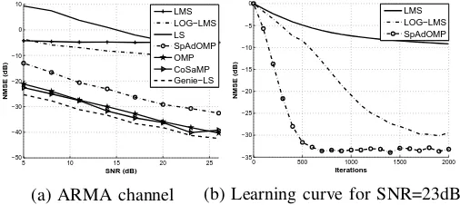
Fig. 1. NMSE of the channel estimates versus SNR on a linear channel

TABLE II

CHOICE OF SPARSE PARAMETERS FOR LOG-LMS

SNR 5-8 11-17 20-26

γa _7×10−4 _8×10−4 _9×10−4

a_{µ= 2×10}−2_{,²= 10}

is used to assess performance.

A. Sparse ARMA channel identification

In the first experiment sparse ARMA channel estimation is considered. The channel memory is My =Mx= 50 and the

channel to be estimated is given by

yn=a1yn−6+a2yn−48+xn+b1xn−13+b2xn−34

where[a1, a2] = [−0.5167−j0.2828,0.1801 +j0.1347]and

[b1, b2] = [−0.5368−j0.9198,1.0719 +j0.0318]. The system

is stable as the roots of the AR part are inside the unit circle. The input sequence is drawn from a complex Gaussian dis-tribution, CN(0,1/5). To reduce the realization dependency, the parameter estimates were averaged over 30 Monte Carlo runs. Program (P`0) is solved by the CoSaMP [1], OMP [8],

[9], log-LMS [12] and SpAdOMP. Moreover, two conventional methods were used, namely, the Least Squares (LS) and the LMS algorithm. The number of samples processed was 500. The sparsity tuning parameter required by the log-LMS is summarized in Table II. The step size for the conventional LMS and the SpAdOMP was set to µLMS = 1×10−2 and

µSpAdOMP = 7×10−2. Note that the choice of the step sizeµ

is made near the instability point of each algorithm to provide the maximum possible convergence speed.

Fig. 1(a) shows the excellent performance match between the Genie LS, CoSaMP and OMP, all of which have quadratic complexity. The LMS, log-LMS and SpAdOMP have an order of magnitude less computational complexity, but only SpAdOMP achieves a performance gain close to Genie LS (9dBless). If we repeat this experiment for a fixed SNR level of 23dB and process 2000 samples, then as shown in Fig. 1(b), log-LMS improves by 20dB; however, it achieves 4dB less performance gain than SpAdOMP.

To demonstrate the support tracking ability of SpAdOMP, we run this experiment and after 300 iterations we set a1 to

zero. This time, since we have a support varying environment,

250 300 350 400 450 500 −0.5

−0.45 −0.4 −0.35 −0.3 −0.25 −0.2 −0.15 −0.1 −0.05 0

Iterations

<

¡

a1

¢

LMS LOG−LMS SpAdOMP

(a) Real part

250 300 350 400 450 500 −0.3

−0.25 −0.2 −0.15 −0.1 −0.05 0 0.05

Iterations

=

¡

a1

¢

LMS LOG−LMS SpAdOMP

(b) Imaginary part

Fig. 2. Time evolution ofa1 signal entry on a linear ARMA channel

5 10 15 20 25

−50 −45 −40 −35 −30 −25 −20 −15 −10 −5 0

SNR (dB)

NMSE (dB)

LMS LS SpAdOMP OMP CoSaMP Genie−LS

(a) NARMA channel

10 15 20 25 −30

−25 −20 −15 −10 −5

SNR (dB)

NMSE (dB)

LMS LOG−LMS SpAdOMP

(b) Nonlinear multipath channel

Fig. 3. NMSE of the channel estimates versus SNR on nonlinear channels

λ is set to λ= 0.8 in SpAdOMP. Fig. 2 illustrates the time evolution of the estimates of a1. We note from Fig. 2, that

the conventional LMS does not take into account sparsity and hence the estimates are nonzero; while log-LMS and SpAdOMP succeed in estimating the zero entries. However, SpAdOMP has a much faster support tracking behavior for the estimation of the zero entries in comparison to log-LMS.

B. Sparse NARMA channel identification

In the second experiment the following NARMA channel is considered

yn=a1yn−50+a2yn2−9+b1xn−8+b2|xn−21|2xn−21

where [a1, a2] = [−0.1586−j0.7064,−0.1428−j0.0478]

and [b1, b2] = [−0.8082−j0.5221,−0.5177 +j0.7131] and

the channel memory isMy=Mx= 50.

The experiment is based on 30 Monte Carlo runs and the input sequence is generated from a complex Gaussian distribution, CN(0,1/4), consisting of 1000 samples. This time, the methods used are CoSaMP, OMP and SpAdOMP, along with the standard LMS algorithm and least squares. The step size parametersµLM S= 6×10−3andµSpAdOM P = 0.3

C. Sparse nonlinear multipath channel identification

In this channel setup, a cubic baseband Hammerstein wire-less channel with four Rayleigh fading rays (two on the liner and two on the cubic part) is employed; all rays fade at the same Doppler frequency of fD = 80Hz with sampling

period Ts = 0.8µs. The channel memory length is equal

to M1 = M3 = 50 (for both the linear and cubic parts)

and the position of the fading rays is randomly chosen. In this experiment, 2000 samples from a complex Gaussian distribution CN(0,1/4) were processed. Fig. 3(b) illustrates that SpAdOMP provides an average gain of 11dB, over the conventional LMS and 5dB over the log-LMS developed in [12].

V. CONCLUSIONS

In this paper, an adaptive algorithm for sparse approx-imations with linear complexity was developed using the underlying principles of existing batch-greedy algorithms. Analytical bounds on the steady-state MSE are obtained, which highlight the superior performance of the proposed algorithm. The proposed algorithm was applied to sparse NARMA identification and in particular to NARMA channel equalization/predistortion. Simulation results validated the su-perior performance of the new algorithm. Future research is focused on blind algorithms for sparse system identification.

APPENDIX PROOF OFTHEOREM1

Note that, unlike CoSaMP, the iterations of SpAdOMP are not applied to a fixed batch of measurements. Hence, we need to revisit the error analysis of CoSaMP taking into account the time variations. Recall that the LMS update forw|Λ(n)(n)

is given by

w|Λ(n)(n) =w|Λ(n)(n−1) (13)

+µφ∗_|Λ(n)(n)¡y(n)−φT_|Λ(n)(n)w|Λ(n)(n−1)

¢

Suppose that the estimate at timen is given byc(n). Let

²1(n) :=kc−c(n)k`2, ²2(n) :=kw|Λ(n)(n)−wo|Λ(n)k`2

(14) where wo|Λ(n) is the optimum Wiener solution restricted to

the set Λ(n), given by

wo|Λ(n):=R−|Λ(1n)r (15)

with R := E{φ(n)φ∗T(n)} and r := E{φ∗(n)y(n)}. One can write

w|Λ(n)(n)−wo|Λ(n)=

³

I|Λ(n)−µφ|Λ(n)(n)φ∗|Λ(Tn)(n)

´

×

½ ¡

w|Λ(n−1)(n−1)−wo|Λ(n−1)

¢

+¡w|Λ(n)(n−1)−w|Λ(n−1)(n−1)

¢

+¡wo|Λ(n−1)−wo|Λ(n)

¢¾

+µφ∗|Λ(n)eo(n) (16)

where eo(n) is the estimation error of the optimum Wiener

filter, given by eo(n) := (y(n)−φT|Λ(n)wo|Λ). Invoking

the Direct-Averaging approximation [20], one can substitute

φ|Λ(n)(n)φ|∗Λ(Tn)(n)withR|Λ(n). Hence,

²2(n)≤(1−µλM)²2(n−1) +µkφ|Λ(n)k2|eo(n)|

+ (1−µλM)

n°_°

w|Λ(n)(n−1)−w|Λ(n−1)(n−1)

° °

`2

+°°wo|Λ(n−1)−wo|Λ(n)

° °

`2 o

(17)

whereλM is the minimum eigenvalue ofR. Here we assume

that the covariance matrix R is non-singular, i.e., λM > 0.

Note that the direct-averaging method yields a reasonable approximation particularly when µ ¿1 [28]. A more direct and rigorous convergence analysis of the LMS algorithm is possible, which is much more complicated [29]. Hence, for the sake of simplicity and clarity of the analysis, we proceed with the direct-averaging approach.

In order to obtain a closed set of difference equations for ²1(n) and ²2(n), we need to express the third and fourth

terms of Eq. (17) in terms of²1(n)and²2(n)(and time-shifts

thereof). First, we consider the third term. Let

δ(n−1) :=w(n−1)−c. (18)

Note that w(n−1) is supported on the index setΛ(n−1). Hence,

°

°_{w|Λ(n)(n−1)−w|Λ(n−1)(n−1)}°°

`2

=°°cΛ(n)∆Λ(n−1)+δΛ(n)∆Λ(n−1)(n−1)

° °

`2

≤°°cΛ(n)∆Λ(n−1)

° °

`2+ °

°_δ(n−1)°°

`2 (19)

where ∆ represents the symmetric difference of Λ(n) and

Λ(n−1). The key here is the fact that the support estimates

Λ(n−1) and Λ(n) contain most of the energy of the true vector c, due to the restricted isometry of the measurement matrix and the construction of the proxy signal. Consider the squared form of the first term in the above equation:

°

°_{cΛ(n)∆Λ(n−1)}°°2

`2 = °

°_cΛ(n)∩Λc_(n−1) ° °2

`2+ °

°_{cΛ(n−1)∩Λ}c_(n) ° °2

`2

≤°°cΛc_(n−1) ° °2

`2+ ° °_cΛc_(n)

° °2

`2 (20)

Hence, °

°_{cΛ(n)∆Λ(n−1)}°°

`2 ≤

√

2 maxn°°cΛc_(n−1) ° °

`2, ° °_cΛc_(n)

° °

`2 o

(21) Lemmas 4.2 and 4.3 of [1] provide the following bound on

kcΛc_(n)k_`2: ° °_cΛc_(n)

° °

`2 ≤γ(n)²1(n−1) +ξ(n) ° °_η0_(n)°_°

`2 (22)

where

γ(n) := δ2s(λ, n) +δ4s(λ, n) 1−δ2s(λ, n)

, ξ(n) := 2

p

1 +δ2s(λ, n)

1−δ2s(λ, n)

, (23) and

η0_{(n) :=D}1/2_{(n)η(n) + Diag}¡_Φ(n)Θ(n)¢ ₍₂₄₎

withΘij(n) :=λn−j−1

¡

ci(n)−ci(j)

¢

, for i= 1,2,· · ·, N andj= 1,2,· · · , n−1. Theeffectivenoise vectorη0_(n)

8 IEEE TRANSACTIONS ON SIGNAL PROCESSING, VOL. XX, NO. XX, MONTH 2010

due to the adaptive update of the proxy signal (in contrast to the batch construction used in the CoSaMP algorithm). Note that the isometry constants δs(λ, n),· · ·, δ4s(λ, n) are

all functions ofn, since the matrixΦ(n)depends onn. If the input sequence is generated by a stationary source, fornlarge enough, one can approximate the covariance matrixRby the exponentially weighted sample covarianceΦ∗T(n)D(n)Φ(n). Similarly, one can approximate r by Φ∗T_{(n)D(n)r(n). In}

this case, we have wo|Λ(n) ≈ b(n), where b(n) is the

exponentially-weighted least squares solution restricted to the index setΛ(n), given by

b(n) :=

(¡

D1/2_(n)Φ(n)¢†

|Λ(n)D

1/2_{(n)r(n), onΛ(n)}

0, elsewhere

(25) Using this approximation, the `2-norm of δ(n−1) can be

bounded as follows: °

°_δ(n−1)°°

`2≤ °

°_{w(n−1)−b(n−1)}°°

`2+ °

°_b(n−1)−c°°

`2

≤²2(n−1) +

°

°_b(n−1)−c°°

`2 (26)

Moreover, using Lemmas 4.2, 4.3, and 4.4 of [1], one can expresskc−b(n)k`2 in terms of²1(n)andη

0_{(n)as follows:}

kc−b(n)k2≤

1

2α(n)²1(n−1) + 1 2β(n)

° °_η0_(n)°_°

`2, (27)

where

α(n) := 2

³

1 + δ4s(λ, n) 1−δ3s(λ, n)

´

γ(n), (28)

β(n) :=p 2

1−δ3s(λ, n)

+ 2³1 + δ4s(λ, n) 1−δ3s(λ, n)

´ ξ(n).

(29)

Denoting kc−b(n)k`2 by ²3(n) and using Eqs. (21), (26),

and (27), one can obtain the following recurrence relation for ²2(n):

²2(n)≤(1−µλM)²2(n−1) +µkφ|Λ(n)k2|eo(n)|

+ (1−µλM)

n°_°

wo|Λ(n−1)−c

° °

`2+ °

°_wo|Λ(n)−c°°

`2

+°°w|Λ(n)(n−1)−w|Λ(n−1)(n−1)

° °

`2 o

≤(1−µλM)²2(n−1) +µ

°

°_φ|Λ(n)°°

`2|eo(n)|

+ (1−µλM)

n

²3(n) + 2²3(n−1) +²2(n−1)

o

+√2(1−µλM) max

n

γ(n)²1(n−1) +ξ(n)kη0(n)k`2,

γ(n−1)²1(n−2) +ξ(n−1)kη0(n−1)k`2 o

(30)

From Lemma 4.5 of Needell et al. [1], one can write

²1(n) :=kc−c(n)k`2 (31)

≤ kc−bs(n)k`2+kbs(n)−c(n)k`2

≤2kc−b(n)k`2+ 4kb(n)−w(n)k`2

≤2kc−b(n)k`2+ 4kwo|Λ(n)−w(n)k`2

+ 4kwo|Λ(n)−b(n)k`2

where the last line of Eq. (31) is obtained from the second line by adding and subtractingwo|Λ(n)fromb(n)−w(n), and

using the triangle inequality. The last term on the right hand side of Eq. (31) denotes the difference between the optimum Wiener solution and the LS solution, both restricted to the index set Λ(n). As mentioned earlier, one can approximate the covariance matrixRby the exponentially weighted sample covarianceΦ∗T(n)D(n)Φ(n), and the correlation vectorrby Φ∗T(n)D(n)r(n). In this case, we havewo|Λ(n)≈b(n), and

hence the contribution of the last term on the right hand side of Eq. (31) to the steady-state error becomes negligible. Also, by construction, the estimatew(n)is supported on the index set

Λ(n). Hence, the second term of Eq. (31) can be identified as 4kwo|Λ(n) − w|Λ(n)(n)k2 = 4²2(n). With the

above-mentioned simplifications, one can arrive at the following set of non-linearly coupled difference equations for ²1(n),²2(n)

and²3(n):

                      

²1(n)≤2²3(n) + 4²2(n)

²2(n)≤(1−µλM)

n

2²2(n−1) + 2²3(n−1) +²3(n)

o

+√2(1−µλM) max

n

γ(n)²1(n−1) +ξ(n)kη0(n)k`2,

γ(n−1)²1(n−2) +ξ(n−1)kη0(n−1)k`2 o

+µ°°φ_|Λ(n)(n)°°_`

2|eo(n)|

²3(n)≤1₂α(n)²1(n−1) +1₂β(n)

° °_η0_(n)°_°

`2

(32) Although the above set of difference equations is sufficient to obtain the error measures ²1(n), ²2(n), and²3(n) for all n,

the solution is non-trivial for general n due to its high non-linearity. However, for large n, it is possible to obtain the steady-state solution. It is easy to substitute ²3(n) in terms

of ²1(n). Also, for large enough n, the arguments of the

max{·,·}operator do not vary significantly withn. Hence, we can substitute the maximum with the second argument. Hence, the steady-state values of ²1(n) and ²2(n) can be obtained

from the following equation:

µ

1−α(n) −4

−(1−µλM)

¡₃

2α(n) +

√

2γ(n)¢ 1−2(1−µλM)

¶ µ ²1(n)

²2(n)

¶

≤°°D1/2(n)η(n)°°_`

2

µ

β(n) (1−µλM)

¡₃

2β(n) +

√

2ξ(n)¢

¶

+µ°°φ|Λ(n)(n)

° °

`2|eo(n)|

µ

0 1

¶

(33)

Note that, the contribution of proxy error term in η0_(n)

becomes negligible for largen, due to the effect of forgetting factor, and the fact that the estimates c(n)do not vary much with n. Hence, we can approximate η0_{(n) by D}1/2_(n)η(n)

for largen. In particular, the asymptotic solution to ²1(n) is

given by:

²1(n).C1(n)

°

°_D1/2_(n)η(n)°_°

`2+C2(n) °

°_φ|Λ(n)(n)°°

`2|eo(n)|

(34) where,

C1(n) :=

4(1−µλM)

³

3

2β(n) +

√

2ξ(n)´ ∆(n)

+

³

1−2(1−µλM)

´ β(n)

∆(n) , (35)

C2(n) := 4µ

and

∆(n) := (2µλM−1)−(5−4µλM)α(n)−4

√

2(1−µλM)γ(n).

(37) Note that a sufficient condition for the above bound to hold is ∆(n)>0.

REFERENCES

[1] D. Needell and J. Tropp, “CoSaMP: Iterative signal recovery from incomplete and inaccurate samples,” Appl. Comput. Harmon. Anal, vol. 26, pp. 301–321, 2009.

[2] W. Dai and O. Milenkovic, “Subspace pursuit for compressive sensing signal reconstruction,”IEEE Trans. Inf. Theory, vol. 55, no. 5, pp. 2230– 2249, 2009.

[3] A. Bruckstein, D. Donoho, and M. Elad, “From sparse solutions of systems of equations to sparse modeling of signals and images,”SIAM

Review, vol. 51, no. 1, pp. 34–81, 2009.

[4] W. Schreiber, “Advanced television systems for terrestrial broadcasting: Some problems and some proposed solutions,” vol. 83, pp. 958–981, 1995.

[5] W. Bajwa, J. Haupt, G. Raz, and R. Nowak, “Compressed channel sensing,” inProc. IEEE CISS, 2008, pp. 5–10.

[6] M. Kocic, D. Brady, and M. Stojanovic, “Sparse equalization for real-time digital underwater acoustic communications,” inProc. IEEE

OCEANS, 1995, pp. 1417–1422.

[7] S. Chen, D. Donoho, and M. Saunders, “Atomic decomposition by basis pursuit,”SIAM J. Sci. Comput., vol. 20, no. 1, pp. 33–61, 1998. [8] Y. Pati, R. Rezaiifar, and P. Krishnaprasad, “Orthogonal matching

pursuit: recursive function approximation with applications to wavelet decomposition,” in27th Asilomar Conf.on Signals, Systems and Com-put., 1993, pp. 40–44.

[9] S. Davis, G.M. Mallat and Z. Zhang, “Adaptive time-frequency decom-positions,”SPIE J. Opt. Engin., vol. 33, no. 7, pp. 2183–2191, 1994. [10] D. Needell and R. Vershynin, “Uniform uncertainty principle and signal

recovery via regularized orthogonal matching pursuit,”Found. Comput. Math, vol. 9, no. 3, pp. 317–334, 2009.

[11] D. Donoho, Y. Tsaig, I. Drori, and J. Starck, “Sparse solution of underdetermined linear equations by stagewise orthogonal matching pursuit,”Submitted for publication.

[12] Y. Chen, Y. Gu, and A. Hero, “Sparse LMS for system identification,”

inProc. IEEE ICASSP, 2009, pp. 3125–3128.

[13] D. Angelosante and G. Giannakis, “RLS-weighted LASSO for adaptive estimation of sparse signals,” inProc. IEEE ICASSP, 2009.

[14] B. Babadi, N. Kalouptsidis, and V. Tarokh, “SPARLS: The sparse RLS algorithm,”submited in IEEE Trans. Signal Process., 2009.

[15] N. Kalouptsidis, G. Mileounis, B. Babadi, and V. Tarokh, “Adaptive algorithms for sparse nonlinear channel estimation,” inProc. IEEE SSP, 2009, pp. 221–224.

[16] E. Cand´es and T. Tao, “Decoding by linear programming,”IEEE Trans.

Inf. Theory, vol. 51, no. 12, pp. 4203–4215, 2004.

[17] M. Figueiredo, R. Nowak, and S. Wright, “Gradient projection for sparse reconstruction: Application to compressed sensing and other inverse problems,”IEEE J. Sel. Topics Signal Process., vol. 1, no. 4, pp. 586– 597, 2007.

[18] I. Daubechies, M. Defrise, and C. Mol, “An iterative thresholding algorithm for linear inverse problems with a sparsity constraint,”Comm.

Pure Appl. Math., vol. 57, no. 11, pp. 1413–1457, 2004.

[19] J. Tropp, “Greed is good: algorithmic results for sparse approximation,”

IEEE Trans. Inf. Theory, vol. 50, no. 10, pp. 2231–2242, 2004.

[20] S. Haykin,Adaptive Filter Theory. Prentice Hall, 1996.

[21] S. Pafka, M. Potters, and I. Kondor, “Exponential weighting and random-matrix-theory-based filtering of financial covariance matrices for portfolio optimization,”Arxiv preprint cond-mat/0402573 (available at

http://arxiv.org/abs/cond-mat/0402573), 2004.

[22] A. M. Sengupta and P. P. Mitra, “Distributions of singular values for some random matrices,”Physical Review E, vol. 60, no. 3, 1999. [23] S. Geman, “A limit theorem for the norm of random matrices,” Ann.

Probab., vol. 8, no. 2, pp. 252–261, 1980.

[24] J. Blanchard, C. Cartis, and J. Tanner, “Compressed sensing: How sharp is the restricted isometry property?”submitted.

[25] N. Kalouptsidis,Signal Processing Systems: Theory & Design. Wiley, 1997.

[26] S. Chen and S. Billings, “Representations of non-linear systems: the NARMAX model,”Int. J. Control, vol. 49, no. 3, pp. 1013–1032, 1989.

[27] S. Benedetto and E. Biglieri,Principles of Digital Transmission: with

wireless applications. Springer, 1999.

[28] H. Kushner,Approximation and Weak Convergence Methods for Random

Processes with Applications to Stochastic System Theory. MIT Press,

1984.

[29] E. Eweda and O. Macchi, “Convergence of an adaptive linear estimation algorithm,”IEEE Trans. Autom. Control, vol. 29, no. 2, pp. 119–127, 1984.

Gerasimos Mileounis (S’04) received the BEng.

degree in Electronic Engineering and Computer Sci-ence from Aston University, UK, and the MSc. (Eng.) degree in Data Communications from Uni-versity of Sheffield, UK, in 2004 and 2005, respec-tively.

He is currently working towards the Ph.D degree in the Department of Informatics and Telecommu-nications at the University of Athens, Greece. His research interests include nonlinear system iden-tification/equalization for communications, higher-order statistics and compressed sensing.

Behtash Babadi (S’08) received the BSc. degree

in Electrical Engineering from Sharif University of Technology, Tehran, Iran and the MSc. in Engineer-ing Sciences from Harvard University, Cambridge, MA, in 2006 and 2008, respectively.

He is currently working towards the PhD degree in Engineering Sciences at the School of Engineering and Applied Sciences, Harvard University, Cam-bridge, MA. His research interests include dynamic spectrum access networks, adaptive signal process-ing and compressed sensprocess-ing.

Nicholas Kalouptsidis(M’82-SM’85) was born in

Athens, Greece, on September 13, 1951. He received the B.Sc. degree in mathematics (with highest hon-ors) from the University of Athens, Athens, Greece, in 1973 and the M.S. and Ph.D. degrees in systems science and mathematics from Washington Univer-sity, St. Louis, MO, in 1975 and 1976 respectively.

He has held visiting positions at Washington University, St. Louis, MO; Politecnico di Torino, Turin, Italy; Northeastern University, Boston, MA; and CNET Lannion, France. He has been an As-sociate Professor and Professor with the Department of Physics, University of Athens. In Fall 1998, he was a Clyde Chair Professor with the School of Engineering, University of Utah, Salt Lake City. In Spring 2008, he was a visiting scholar at Harvard university. He is currently a Professor with the Department of Informatics and Telecommunications, University of Athens. He is the author of the textbookSignal Processing Systems: Theory and Design

(New York: Wiley, 1997) and coeditor, with S. Theodoridis, of the book

Adaptive System Identification and Signal Processing Algorithms(Englewood

Cliffs, NJ: Prentice-Hall, 1993). His research interests are in system theory and signal processing.

Vahid Tarokh (M’97-SM’02-F’09) received the

Ph.D. degree in electrical engineering from the Uni-versity of Waterloo, Waterloo, ON, Canada, in 1995.

He is a Perkins Professor of Applied Mathematics and Hammond Vinton Hayes Senior Fellow of Elec-trical Engineering at Harvard University, Cambridge, MA. At Harvard, he teaches courses and supervises research in communications, networking and signal processing.