Toward a unifying framework for evolutionary processes.

Toward a unifying framework for evolutionary processes

Tiago Paixão

a,n

, Golnaz Badkobeh

c

, Nick Barton

a

, Do

_ğ

an Çörü

_ş

b

, Duc-Cuong Dang

b

,

Tobias Friedrich

d

, Per Kristian Lehre

b

, Dirk Sudholt

c

, Andrew M. Sutton

d

,

Barbora Trubenová

a

a

Institute of Science and Technology, Am Campus 1, A3400 Klosterneuburg, Austria b_{University of Nottingham, UK}

c_{University of Sheffield, UK} d

Hasso Plattner Institute, Potsdam, Germany

H I G H L I G H T S

_{A unifying framework for evolutionary processes.}

_{Formalizing the defining properties of the different kinds of processes:}

○Variation operators (mutation and recombination).○Selection operators.

Formalizing several common examples of these operators in terms of our framework. Proving that these common operators respect the properties that we define for their class. Casting several classical models and algorithms from bothfields into our framework.

a r t i c l e i n f o

Article history:

Received 27 November 2014 Received in revised form 8 July 2015

Accepted 15 July 2015 Available online 26 July 2015

Keywords:

Population genetics Evolution

Evolutionary computation Mathematical modelling

a b s t r a c t

The theory of population genetics and evolutionary computation have been evolving separately for nearly 30 years. Many results have been independently obtained in bothfields and many others are unique to its respective field. We aim to bridge this gap by developing a unifying framework for evolutionary processes that allows both evolutionary algorithms and population genetics models to be cast in the same formal framework. The framework we present here decomposes the evolutionary process into its several components in order to facilitate the identification of similarities between different models. In particular, we propose a classification of evolutionary operators based on the defining properties of the different components. We cast several commonly used operators from both fields into this common framework. Using this, we map different evolutionary and genetic algorithms to different evolutionary regimes and identify candidates with the most potential for the translation of results between thefields. This provides a unified description of evolutionary processes and represents a stepping stone towards new tools and results to bothfields.

&2015 The Authors. Published by Elsevier Ltd. This is an open access article under the CC BY-NC-ND license (http://creativecommons.org/licenses/by-nc-nd/4.0/).

1. Introduction

Evolutionary computation and population genetics share a com-mon object of study, the evolutionary process. Population genetics tries to understand the evolution of natural populations while evolu-tionary computation focuses on designing and understanding artificial evolutionary processes used for solving optimization problems. Bothfields have developed independently, with very little interaction between them.

Population genetics (PG) studies how evolution is shaped by basic forces such as mutation, selection, recombination, migration among sub-populations, and stochasticity; it forms the core of the modern understanding of evolution (the so-called“modern synth-esis”). PG has a long tradition of mathematical modelling, starting in the 1920s with the pioneering work of Fisher, Wright, Haldane and others, and is now a highly sophisticated field in which mathematical analysis plays a central role. Early work focussed on simple deterministic models with small numbers of loci, aiming Contents lists available atScienceDirect

journal homepage:www.elsevier.com/locate/yjtbi

Journal of Theoretical Biology

http://dx.doi.org/10.1016/j.jtbi.2015.07.011

0022-5193/&2015 The Authors. Published by Elsevier Ltd. This is an open access article under the CC BY-NC-ND license (http://creativecommons.org/licenses/by-nc-nd/4.0/).

n_{Corresponding author.}

E-mail addresses:[email protected](T. Paixão),[email protected](G. Badkobeh),[email protected](N. Barton),

[email protected](D. Çörüş),[email protected](D.-C. Dang),[email protected](T. Friedrich),[email protected](P.K. Lehre),

at understanding how the change in genotype frequencies in a population was affected by basic evolutionary forces. It has since branched out to investigate topics such as the evolution of sexual reproduction, the role of environmental fluctuations in driving genetic change, and how populations evolve to become indepen-dent species. Almost all current PG models are restricted to the simplestfitness landscapes. Since naturalfitness landscapes are likely to be far more complicated, indeed too complicated to ever be measured completely, there is a need for a theory that describes the speed of adaptation over a broad range of landscapes in terms of just a few key features.

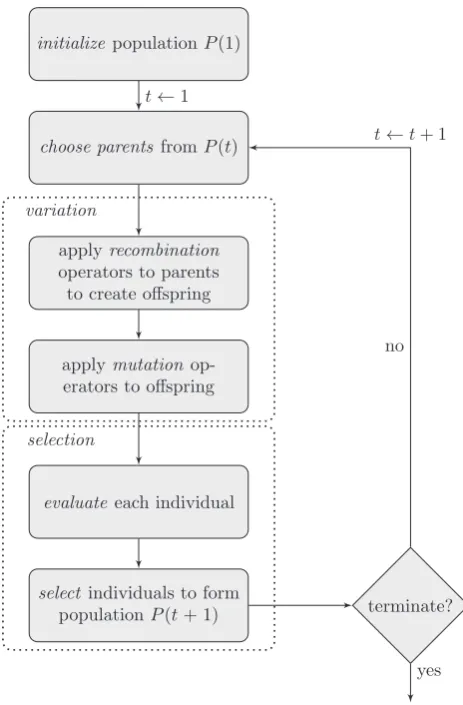
In evolutionary computation (EC), theevolutionary algorithmis the basic object of study. An evolutionary algorithm is a computa-tional process that employs operators inspired by Darwinian principles to search a large state space. The basic scheme of an evolutionary algorithm is depicted in Fig. 1. However, specific concrete evolutionary algorithms differ in the details of each step, for example how elements are selected for reproduction or survival, or which variation operators are used. Evolutionary algorithms typically deal with finite populations and consider classes offitness functions, in contrast with PG that mostly deals with specific instances. Moreover, these classes can be of arbitrary complexity, such as in the case of combinatorial optimization, again in contrast with PG, where mostly the simplest landscapes are considered.

As can be seen, the questions and approaches both_fields take are very different. However, the underlying processes share strik-ing similarities. The basic processes of variation and selection, as proposed by Darwin, seem to be required, though these can appear in many different forms. Is there something general that could be said about evolutionary processes? Can we compare different evolutionary processes in a common framework, so that we can identify similarities that may not be obvious? What are the general features of an evolutionary process? What are the required properties of operations such as mutation or recombination? In fact, what is an evolutionary process?

In order to tackle these questions, we propose a general framework that is able to describe a wide range of evolutionary processes. The purpose of such a framework is to enable compar-isons between different evolutionary models. We require this framework to be modular, so that different components of the evolutionary process can be isolated and independently analysed. In nature, this separation between the different processes does not necessarily exist. However, even when the different processes become entangled with each other, if the dynamics are slow enough, as is typical in natural systems, their relative order in the life-cycle becomes largely irrelevant. This will allow us to identify evolutionary regimes and evolutionary algorithms that are similar, allowing translation of results between the two fields. Furthermore, comparing related but different models and algo-rithms will allow us to disentangle the relative role of different processes or choices of process for the speed of adaptation.

A general framework for evolutionary models that is able to integrate models from both EC and PG in a way suitable for comparison should display the following properties:

The framework should be able to represent the vast majority of different evolutionary processes in a common mathematical framework.

The framework should be modular with respect to the different mechanistic processes of evolution (mutation, selection, etc.) and describe evolutionary processes as compositions of these processes.

It should be able to describe bothfinite and infinite populations and make it easy to relate infinite population models to their stochastic counterparts.

In this report we propose such a framework and we show that by instantiating several evolutionary processes within this frame-work we can find unsuspected similarities between different evolutionary algorithms and evolutionary regimes.

There have been several attempts at creating a general frame-work to describe different models in both PG and EC (Altenberg,

1995; Affenzeller, 2005), although none that created a general

framework to describe different models in both. In the following section we review some of these other attempts at general models of evolution.

2. Related work

2.1. Population genetics models

In population genetics the dynamics of evolution are typically described in terms of the dynamics of allele or genotype frequencies. In a certain sense, this type of framework is a general model of evolution, albeit not a very useful one, because of its generality. It is akin to saying that the theory of differential equations is a general model of dynamics. However, there have been a few attempts at formalizing this dynamical process into more structured forms, suitable for comparison between differ-ent models.

Lewontin (1964)first introduced a general model of evolution

[image:2.595.319.551.55.408.2]

for deterministic systems that is cast in terms of frequencies of genotypes. In this model, a basic recursion is defined that describes

a canonical evolutionary system:

pðtþ

_Δ

tÞ ¼ X y;zAG

Tðx’y;zÞwðy;zÞ w2 pðyÞpðzÞ;

wherep(x) represents the genotype frequency over the search space S,w(x) represents thefitness of genotypexandTðx’z;yÞis the so-called“genetic operator”that represents the probability (or rate) of generating genotypexfrom parentsyandzdue to the combined action of genetic operators (mutation, recombination, etc.). If reproduction is asexual and only selection is acting on the popula-tion, this operator will have a simple form, while more complex transmission will yield less simple forms. This model has been used to obtain a number of results for particular instances of the T operator (Slatkin, 1970; Cavalli-Sforza and Feldman, 1976). In order to unify several models of genes controlling transmission processes,

Altenberg (1984) utilized and gave the first analysis of general

transmission operators, which has since then be extended and analysed in much broader contexts (Altenberg and Feldman, 1987;

Altenberg, 2010, 2012).

In the same spirit as the previous model, Barton and Turelli

(1991) and Kirkpatrick et al. (2002) proposed a model that

structures the different components of the evolutionary process. While the general form of Lewontin's model introduced by

Altenberg (1984)leaves the transmission in general form so that

it can represent any model of reproduction, here the focus is on allele frequencies and their associations between different loci. In the deterministic case, this model amounts to a change of coordinates that facilitates algebraic manipulation. When the population is at “linkage equilibrium”, or close to it, the model takes an especially simple form. This framework uses the notion of “context” in order to model many different situations, from structured populations (where the context is the physical location) to epistasis (where the context is the genetic background) and tracks associations between different sets of genes. This model makes it very easy to deal with multi-locus systems, from an algebraic point of view, and it has been used to address several questions, for example regarding the role of epistasis in different demographic conditions (Turelli and Barton, 2006; Barton and

Turelli, 2004).

Both previous examples of a general framework focus on the dynamics of genotype or allele frequencies and are appropriate for analysis of different models. However, both frameworks are very tailored for biological systems, where selection assumes a parti-cular form. For this reason, even though some modifications could be implemented, we believe that they lack some of theflexibility required to compare the structure of models in EC and PG.

Another type of general framework is exemplified by the approach that quantitative genetics takes: a purely phenotypic description of the evolution of some continuous trait (Falconer and

Mackay, 1996). In this approach, a population is characterized by

its genetic variance and its contribution to _fitness. Typically, a decomposition of this genetic variance is used that partitions it into components that can contribute to the advance of the population with different relative strengths. This approach is only useful when (at least some) genetic recombination is assumed. Different processes (such as mutation) can be included in this type of framework by calculating their contribution to the genetic variance of the population. The fundamental relation in this framework is the so-called breeder's equation:R¼

_β

VA, whereR is the one generation increase of the mean of a given trait,

β

is the selection gradient, andVAis the additive genetic variance of the

population. More generally, one can write recursions for all moments of the distribution of phenotypes in the population. Different selection schemes can be cast into this framework, which has been of considerable value in animal breeding. In particular,

results concerning the ultimate increase in a trait given a certain initial standing variation in a population, or optimal selection strategies were obtained under this framework. One drawback of this approach is that the recursions do not close, since the change in one of the moments depends on the next highest order moment. The downside of this framework is that it absolutely ignores the dynamics of the underlying genes and their relation-ships, and models all processes as effects on the dynamics of the genetic variance (or other statistical descriptors) of the population. This makes this framework unable to tackle questions about the optimality of different processes or about dynamics of genes or importance of genetic architecture. However, this approach is related to the previous one, by Barton and Turelli: if one rewrites the recursions in terms of allele frequencies one gets a form very close to the one these authors obtained.

An even more general framework of evolution comes in the form of the Price equation (Price, 1970, 1972). This equation assumes a population of replicating entities and considers the mean increase in some arbitrary property of these entities, which can be a trait, orfitness itself. If we assume that each individual in the population has a relative number of offspringwi¼ni=Pjnj, then the change of the mean of the traitzin one generation will be w

Δ

z¼Covðwi_;ziÞþE½wi

Δ

zi. This approach is very general and related to the approach taken by quantitative genetics. Because the nature of this trait is not specified and the replicating entities are also abstract, this type of approach has been used to derive results in social evolution, and has influenced many otherfields. The generality and simplicity of the Price equation make it very useful in comparing different mechanistic models and reduce them to their most fundamental characteristics.

Other general approaches to evolution have also been attempted. For example, genetic algebras (Schafer, 1949) were a

field of active research some decades ago, but progress has slowed down considerably in later years. This approach identifies regula-rities in genetic inheritance rules with operations in mathematical algebras and describes the evolution of these populations. Genetic algebras are highly mathematical; their focus is in describing the consequences of different inheritance rules for the evolution of populations and seem less appropriate to describe other genetic operations such as mutation.

2.2. Evolutionary computation

Evolutionary algorithms (EAs) represent a category of algo-rithms which mimic artificial evolution of candidate solutions in order to solve or to produce approximate solutions to design and optimisation problems. There exist countless EA variants, often characterised by different principles inspired by nature or related to different problem domains. This made the attempts to unify models of EAs often scattered, or limited to some specific branch of computer science.

De Jong (2006)characterises a Darwinian evolutionary system

Primarily inspired by the Simple Genetic Algorithm (SGA),Vose

(1999a) has summarised many heuristic searches into a single

framework, the so-called Random Heuristic Search. In this frame-work, a heuristic search can be seen as a collection/population of initial search pointsP0from the set of all possible search pointsG wherejGj ¼2n, together with some transition rule

τ

to produce a new population from a given one. The search is then described by the series of transformationP0-τP1-τ P2-τ ⋯. The analyses of such a model require the characterisation or localisation of a given population, e.g. the current population, in the space of all possible populations. This is done with population vectors: a population vector ofPis a real vector of lengthnand each component of the vector corresponds to the frequency of a specific element ofGinP. Thus the set of all possible populations is the simplex

Λ

¼ f〈p1;…;pn〉∣p1þ⋯þpn¼1g. This is similar to the typical descriptions of populations used in PG, and detailed in the previous section. The advantage of this representation is that it is not necessary to specify the population size, e.g. it is easy to make assumptions about large or infinite populations. Several theoretical results, such as convergence rates, were deduced based on the properties of the admissible transition rules for large populations (seeVose, 1999afor a summary).

From a geometrical perspective,Moraglio (2007)has proposed a unifying framework to look at evolutionary algorithms. The framework requires a geometric structure to be identified on the space of solutions or the genotype space. Such a structure can be discovered byfinding a metric distance measure between solu-tions, e.g. satisfying the symmetry and the triangle inequality. Based on the metric distance, several geometric objects, such as segments,ballsorconvex objects, can be defined. Then evolutionary operators can be categorised into geometric and non-geometric ones with respect to the distance measure. For example, a geometric recombination operatorof two parent solutions should guarantee that the offspring will lie on the segment defined by the parents. From that the population can be represented by a certain “shape_”, e.g., theconvex hullenveloping the individuals, and the algorithm evolves by modifying this shape. Several theoretical results, such as the runtime, can be deduced from the geometric properties of the operators and the search space (see Moraglio, 2011). Many evolutionary operators are geometric under an appropriate metric distance measure, while for others it is unknown if such a distance measure exists. In addition, the global characteristic, e.g. non-zero probability of moving the population to any region of the search space in one step, of many variation operators is sometimes uncovered by geometric arguments

(Moraglio and Sudholt, 2012). In related work, Droste and

Wiesmann (2000)proposed a set of design guidelines for

evolu-tionary algorithms. These included a set of desirable properties to be met by the recombination and mutation operators, as well as the genotype–phenotype mapping. Some of these properties are similar to those described inSection 4of this paper.

Rabani et al. (1998) and Rabinovich et al. (1992) suggested

modelling genetic algorithms by quadratic dynamical systems, a stochastic formalism which generalises Markov chains, much in the same way asLewontin (1964),Slatkin (1970), andAltenberg

(1984)in PG. Although powerful, this formalism has seen limited

adoption, partly because starting from certain distributions, sam-pling from a quadratic dynamical system at anyfixed time belongs to the class of PSPACE-complete problems (Arora et al., 1994), which are considered intractable.

As a branch of computer science, evolutionary computation is also concerned withcomputational complexitywhich attempts to characterise the inherent difficulty of computational problems when solved within a given model of computation, such as the Turing Machine model. Black box models have been developed in EC to capture the essential limitations of evolutionary algorithms

and other search processes. In black box models, an adversary picks a functionf:f0;1gn

-Rfrom a class of functionsF, which is known to the algorithm. The chosen functionfis unknown to the algorithm, but the algorithm can query the function valuef(x) for any bitstringxAf0;1gn

. The goal of the algorithm is to identify a bitstring xn_Af0;1gn

that maximises f. The unrestricted black-box model (Droste et al., 2006) imposes no further restrictions on the algorithm. In the ranking-based black-box model, the algorithm can only query for the relative order of function values of search points (Teytaud and Gelly, 2006; Doerr and Winzen, 2011). In the memory-restricted black-box model (Droste et al., 2006; Doerr

and Winzen, 2012), the algorithm has limited memory. The

unbiased black-box model (Lehre and Witt, 2012) puts restrictions on how new search points can be generated. This model defined unbiased variation operators of any arity, but only unary variation operators (such as mutation operators) were analysed initially. Later, higher arity operators (such as crossover) were also analysed

(Doerr et al., 2011), as well as more general search spaces (Rowe

and Vose, 2011). This approach is appropriate to estimate the

fundamental limits of an evolutionary process in a given class of functions. However, it seems unnatural to use it to decompose an evolutionary process into its fundamental sub-processes.

Reusability and easy implementation are often concerns of the users of evolutionary algorithms, both practitioners and research-ers. Many efforts have been made to address this issue from the perspective of software engineering. In fact, many evolutionary operators have the same type of input and output. In addition, they can handle the elements of the input at a very abstract level and can be unified. From the user perspective the implementation of an evolutionary algorithm on a specific problem is boiled down mostly to the selection of solution representation and the defi ni-tion of the evaluani-tion procedure. Many software libraries for evolutionary algorithms are based on this principle, some exam-ples are ECJ (Luke), GALib (Wall) or ParadisEO (Cahon et al., 2004,

INRIA). Generally speaking, some implicit unified models exist in

those frameworks. Our framework is in parts inspired by FrEAK, the Free Evolutionary Algorithm Kit (Briest et al., 2004), a free toolkit for the creation, simulation, and analysis of evolutionary algorithms within a graphical interface. Evolutionary algorithms in FrEAK are represented by operator graphs: acyclic flow graphs leading individuals through various nodes. The nodes represent evolutionary operators like mutation, recombination, and selec-tion. They process the incoming individuals and propagate the result of an operation through their outgoing edges. Every gen-eration, the current population is led through the algorithm graph from a start node towards afinish node where the new population is received. This modular approach allows the representation of a wide variety of evolutionary processes that differ in the composi-tion and sequence of operators applied.

3. A unifying framework for evolutionary processes

In a general sense, any evolutionary process (natural or artificial) can be seen as a population undergoing changes over time based on some set of transformations. Formally, given afinite set G, called thegenotype space or genospace, an evolvingfinite population is a sequence

Pð1Þ;Pð2Þ;…;PðtÞ;…

ð Þ;

where eachPðtÞAGk

Pðtþ1Þin any evolutionary process. Specifically, we are interested in characterizing the random mapping1

_ψ

_:Gk_-Gk_{such that} Pðtþ1Þ ¼

_ψ

ðPðtÞÞ:

Our approach decomposes

ψ

into a collection of modular operators that each has a distinct and elementary role in the evolutionary process. Typically, these operators act on sequences ofG. These sequences are typically constructed from the elements ofP(t), from the output of operators, and from the concatenation operator. Given twofinite sequencesxAGℓ_andyAGm

, we denote theconcatenationofxandyasx[y, which is an element ofGℓþm_. Given two operators G1:Gℓ-Gn and G2:Gm-Gℓ that act on sequences ofG, we denote thecomposition of G1 and G2 as the operatorðG1○G2Þ:Gm-Gn≔x↦G1ðG2ðxÞÞ.

Sequences describe finitepopulations and operators typically perform stochastic operations on the elements of these sequences (the individuals in the population). The outcome of the action of these stochastic operators can also be described by a probability distribution of potential outcomes, which can be used to induce a different level of description of the evolutionary process. This suggests that an evolutionary process can be defined as a trajec-tory through a space ofdistributions S(the space of all genotype frequency distributions, represented by the jGj 1 dimensional simplex). Formally, we can view these operators acting in this distribution space

Dð1Þ;Dð2Þ;…;DðtÞ;…

ð Þ:

EachD(t) is an element of a set of distributions over populations. Analogously, we might have some transformation

Dðtþ1Þ ¼

_ϕ

ðDðtÞÞ;

where

ϕ

can be decomposed into modular operators that are homologous to the operators in

ψ

(Fig. 2). The distribution at time tþ1 might even depend somehow on the state of the finite population at timet. In some algorithms and models, the finite population of sizekat timetþ1 can be constructed by samplingk elements from the distribution at time tþ1. We denote this sampling operator as

β

k. Given any distribution DAS over the set of genotypes, we can obtain a concrete population of sizekby applying the sampling operator

β

k:S-G

k

defined as

β

kðDÞ≔ðXiÞiA½k whereX1;…;XkD:

wheredenotes that all theXkare independently and identically

distributed as the distributionD. An operatorG:Gk_{-Gacting on} genotypes, can be “lifted” to a mapping Gb:S-S between dis-tributions as follows. Given any distributionDAS, we defineGbðDÞ to be the distribution where

PrðZ¼z∣ZGbðDÞÞ≔PrðGðX1;…;XkÞ ¼z∣X1;…;XkDÞ:

To make this concrete, consider an operator that acts on bitstrings andflips each bit with probabilityp. When acting on a de_finite bitstring, sayg1¼ð0;1Þ, this operator will create bitstrings g0¼ð0;0Þ, g2¼ð1;0Þ, and g3¼ð1;1Þ with probabilities

ψ1

j0¼ ð1pÞp,

ψ1

j2¼p2, and

ψ1

j3¼pð1pÞ. In this example DðtÞ ¼ð0;1;0;0Þ, where the positions refer to the probabilities of g0, g1, g2 and g3, and, under the action of this operator, Dðtþ1Þ ¼ ð1pÞp;ð1pÞ2

;p2_;ð1pÞp

. The probabilities that the operator produces any genotype, when applied to any genotype represents the“lifting”of this operator. Anyfinite population can

be described as a frequency distribution of genotypes and the action of this operator on a population can be described by convolving this frequency distribution with the“lifted” operator on each of the individual genotypes. This produces a probability distribution on the genotype produced by the operator, given that we are choosing the individual it acts on uniformly from the population. This distribution can then be used to produce a new population by sampling from it.

“Lifted operators”can also be seen as the“infinite population size_” version of the stochastic operator, since when applied to a frequency distribution, they produce a frequency distribution of the expectation (a statistic) of this operator. This is done by the map

α

:Gk

-S(Fig. 2). Sampling operations are the only ones that

explicitly project from the distribution space into the populations space. Some types of operators explicitly involve some kind of sampling operation (e.g. selection operators, discussed below), but can always be written as a combination of a“lifted”/deterministic operator and a sampling operation.

Some models operate only at the level of populations, others only at the level of distributions and others shift between the levels. For a complete picture, we model the evolutionary process at both levels by two sequences, one in the space of populations, and one in the space of distributions. Our framework then characterizes and classifies the components that comprise the various transformations between these two sequences, and their roles in de_fining the evolutionary process. This is described in

Fig. 2.

3.1. The nature of evolving entities

In each iteration of an evolutionary process, which is called a generation, the operators that comprise

ψ

,

ϕ

,

β

k, and

α

work together to act on the current population to generate a new one. Each operator acts directly on the genotype space, but some operators also depend on information that lies in a broader phenotypespace. Each individual of a population is mapped into this phenotype space, and this transformation is called the genotype–phenotype mappingin population genetics. In evolution-ary computation, the transformation corresponds to the decoding process from genome to solution, e.g. in an indirect encoding scheme. Another transformation will act on this set of phenotypes and assign to each individual of the population a“reproductive value”, which can be seen as a probability of survival or inclusion into the next generation. For evolutionary algorithms, the phenotype-fitness mapping is broken down into evaluation of theobjective functionand various ways to select individuals for the next generation and the next reproduction based on the obtained objective values. Finally, a population that was funnelled through this process is transformed by variation operators, produ-cing a new population.

The two mapping processes are depicted in Fig.3. The genotype and phenotype spaces are sets_G and_P respectively. The geno-type–phenotype mapping is a function

φ

from G to P. An individualg is an element ofG that has phenotype

φ

ðgÞ, which in turn as objective valuefð

φ

ðgÞÞ. A populationPis a sequence of elements ofG, e.g.PAGk _{for a population of sizek.}

The dual representation of individuals as pairs of genotypes and phenotypes immediately suggests the existence of two kinds of operators: operators that act primarily on genotypes and operators that act primarily on phenotypes. Those are the basic ingredients in Darwin's theory of natural evolution: variation and selection. As such, it is natural to make the distinction between these two kinds of operators and to identify them with operations that act on these two spaces. We can then see evolution as a series of applications of these two kinds of operators. Because evolu-tionary algorithms are very diverse in their mode of operation, the 1

Implicitly, we assume an underlying probability spaceð_Ω;F;PrÞwhereΩis a sample space, F is aσ-algebra on Ω, and Pr is a probability measure onF. Furthermore, we assume thatðGk_{;EÞis a measurable space. The mappingψ is}

formally a functionψ:Gk_Ω-Gk_{such thatψ}

xðωÞ≔ψðx;ωÞisðF;EÞ-measurable

for anyfixedxAGk_{. Conversely, the functionψ}

relative order and frequency with which any of these operators act on the population are largely arbitrary. Hence, various evolution-ary processes can be conceived by specifying different orders, e.g. in which variation operators act_first and selection last, or even schemes in which different kinds of selection or variation opera-tors act at different stages of the process and populations are built from the union of the result of the operation of different operators. This will be detailed when we instantiate a particular evolutionary process in our framework inSection 5.

At the same time, this dual nature of evolutionary objects (genotype and phenotype) immediately allows one to deduce some properties of theG andPspaces. Even though bothGand P may have natural metrics the relevant metric distance for evolution is dependent on both the way genotypes change (mutation) and the mapping function between the two spaces

φ

. How close two genotypes are depends on the mutation operator

(Altenberg, 1995), on how likely or dif_ficult it is to turn one into

the other, whereas how close two phenotypes are depends on how close the closest genotypes that produce that pair of phenotypes are from each other. From this we see that even though we started by defining both genotype and phenotype spaces as sets, in reality, in the context of an evolutionary process, they can be imbued with more structure. Typically, the cardinality of G is larger than of Pðj jGZj jÞP . This is because the genotype–phenotype mapping is typically redundant, meaning that many genotypes map to the same phenotype. This can lead to some phenotypes having a bigger pool of genotypes that map to them and, consequently, even if the change at the genotypic level is isotropic, the change at the phenotypic level is not necessarily so. This is similar to the notion ofphenotypic accessibilitythat Stadler et al. have proposed

(Stadler et al., 2001).

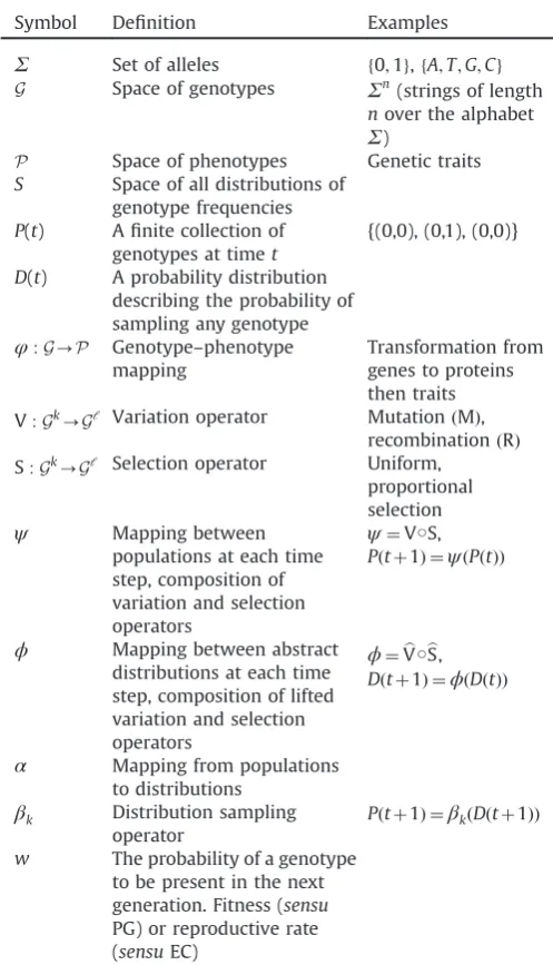
In the following section, we define the evolutionary operators and formalise their properties. The following symbols will be used for these purposes.

Symbol Definition Examples

Σ

Set of alleles f0;1g,fA;T;G;Cg G Space of genotypes

_Σ

n

(strings of length nover the alphabet

Σ

)

P Space of phenotypes Genetic traits S Space of all distributions of

genotype frequencies P(t) Afinite collection of

genotypes at timet

{(0,0), (0,1), (0,0)}

D(t) A probability distribution describing the probability of sampling any genotype

φ

:G-P Genotype–phenotype

mapping

Transformation from genes to proteins then traits V:Gk

-Gℓ Variation operator MutationðMÞ, recombinationðRÞ S:Gk_-Gℓ Selection operator Uniform,

proportional selection

ψ

Mapping between

populations at each time step, composition of variation and selection operators

ψ

¼V○S, Pðtþ1Þ ¼

_ψ

ðPðtÞÞ

ϕ

Mapping between abstract distributions at each time step, composition of lifted variation and selection operators

ϕ

¼Vb○bS, Dðtþ1Þ ¼

_ϕ

ðDðtÞÞ

α

Mapping from populations to distributions

β

k Distribution sampling operator

Pðtþ1Þ ¼

β

kðDðtþ1ÞÞ

w The probability of a genotype to be present in the next generation. Fitness (sensu PG) or reproductive rate (sensuEC)

4. Evolutionary operators

In order to be able to compare and contrast different evolu-tionary algorithms and models (processes) we need to break down these processes into their different components. We typically define operators as acting onfinite populations. Given a current population P(t), the population in the next generation becomes Pðtþ1Þ ¼

ψ

ðPðtÞÞ. As pointed out above, the distinction between variation at the genotypic and the phenotypic levels makes it natural to associate different operators that operate at these different levels, variation and selection operators, respectively.

4.1. Selection operators

[image:6.595.51.286.56.156.2]

Selection operators can be used to choose individuals for either reproduction, the so-called parent selection, or for survival, e.g. deciding which individuals will be kept in the next generation. As Fig. 2.The evolution process represented as a sequencefDðtÞ:tANgof

distribu-tions and a sequencefPðtÞ:tANgof vectors inGk _{(concrete populations) that}

[image:6.595.311.560.98.532.2]

depend on each other via various mappings. Each mapping is constructed by a composition of evolutionary operators that we characterize and classify in this work.

Fig. 3.A basic sequence of operations leading to a selectable population. A

population distributed over the genotype spaceðGÞis assigned phenotype values

a consequence, they model competitiveness in different types of populations. Nevertheless, the selection operators are defined in the same way: they have access to the phenotypic information (or the mappings

φ

) and transform one population to another, i.e.,

Sφ:Gk-Gℓ:

For simplification, we also omit

φ

from the notation. Selection operators do not introduce variation (in the sense of new geno-types), hence their defining property is that every element in the output population should be the exact copy of an element from the input population. Formally,

8gAG ifgASðPÞthengAP: ðS1Þ

Selection operators guide the search by taking advantage of local information in the fitness function w. To describe this process, the mapping

φ

first associates to each genotype ga set of

τ

measurable phenotypic traits, denoted by ð

_φ1

ðgÞ;…;

φ

τðgÞÞARτ. To each of these sets of traits theobjective functionassociates a value, representing the adaptiveness of the combination of the traits through interactions with the environ-ment. The selection operators will then sample individuals to be represented in the next generation based on the value of the objective function. This process effectively assigns each individual a probability that it will be represented in the next generation or a reproduction rate. This is typically what is meant in PG as“fitness” ðwÞ. It is common in both_fields to collapse some of these steps into one, effectively assuming the identity operator for one or more of the transformations we just described. In population genetics,w could be arbitrarily chosen, depending on the objective of the study. In evolutionary computation, the phenotypic traits ð

_φ1

ðgÞ;…;

φ

τðgÞÞ are typically collapsed to the objective function, which is multiple for

τ

41 or single for

τ

¼1, andwis rather a property deduced from the selection mechanism. However, it should be noted that even implicitly most models still define a phenotype which is distinct from the objective function. For example, in EC, it is common practice to analyze the performance of EAs on functions of unitation (functions that take as argument the number of 1 s in the bitstring). In this case, it is natural to call the number of 1 s the phenotype and the function of unitation the objective function. Very similar models of phenotype - objective function pairs exist in biology.

It should be noted that the distinction we make here between variation and selection operators, and the different properties we will require of them, resolve some philosophical questions regard-ing the concept of“fitness”. In PG,fitness is typically defined as the “the expected number of offspring of an individual”, while in EC

fitness it is the value of the objective function in question. Even though related, the subtly different meanings of this concept in the two communities still lead to much confusion. Because the expected number of offspring of a given genotype can change due to factors that have nothing to do with selection, the concept is hard to operationalize in the real world. In fact, in theoretical population geneticsfitness is often defined as a function of some underlying genotype and, in this case, it has exactly the same meaning as in EC, which has lead to confusion even within the PG community. In our framework,fitness,sensuPG, can be obtained directly from the selection operators and consists of a derived property from the selection operator used (and the functions it takes as parameters). In EC, this sense offitness has been called the reproduction rate (Table 1).

The following operators are commonly used in evolutionary algorithms (assuming maximization problems) and by their defi -nition satisfying(S1).

Uniform selection: Under this selection operator, denoted by SUnif, each individual of the output population has an equal probability of being a copy of each individual from the input

population. Formally,

SUnifððg1;…;gkÞÞ ¼ ðg01;…;g0ℓÞs:t:Pr g0i¼gj

¼1=k

for alliA½ℓ; jA½k:

There are two ways to implement this selection operator. The standard way, denoted by SUnif, is independent uniform sampling g0_iUnifððg1;…;gkÞÞ with replacement. Another way, which is denoted by SnUnif, is to do the sampling without replacement. In this variant, the outcomes of the sampling are no longer indepen-dent butexchangeable, hence they preserve the required property on the equal probability 1=k.

Proportional selection: This selection operator is defined similar to uniform selection, except that instead of having an equal probability for each individual, the probability of choosing a particular individual is proportional to the value of an objective functionfon that individual. Formally,

SPropðfÞððg1;…;gkÞÞ ¼ ðg01;…;g 0

ℓÞ s:t:Pr g0i¼gj

¼ fðgiÞ Pk

j¼1fðgjÞ for alliA½ℓ; jA½k:

Note that in PG,fis replaced by thefitness functionw, which gave the original name for the selection mechanism. In implementa-tions, g0_i is independently sampled from a custom distribution defined by the probabilitiesfðgiÞ=Pk

j¼1fðgjÞ.

Tournament selection: This selection operator, denoted by STourðf;mÞ, performs a number of experiments, called tournaments,

with respect to some objective functionf. In those tournaments, an individual with the highest value offis selected from a randomly chosen subset ofPof sizem. Formally, STourðf;mÞ:Gk-Gℓis defined as

STourðf;mÞððg1;…;gkÞÞ ¼ ðg01;…;g 0

ℓÞ s:t:g0i¼arg max fðxÞ f

x_APig

for alliA½ℓ where; Pi¼SUnifðmÞððg1;…;gkÞÞ:

Here SUnifðmÞððg1;…;gkÞÞ is the uniform selection described above with the size of the output population explicitly given asm. For mrk, the use of SnUnifðmÞððg1;…;gkÞÞ instead implies the variant SnTourðf;mÞof the selection.

Truncation selection: Under this selection operator, denoted by STruncðf;m;nÞ, each output individual is uniformly selected from a

fixed fraction, for example 10%, of thefittest individuals defined by a measure fof the input population. Formally, an ordering of a population is defined as

SSortðfÞððg1;…;gkÞÞ ¼ ðgrð1Þ;…;grðkÞÞ s:t:fðgrð1ÞÞZ⋯ZfðgrðkÞÞ:

The ordering is entirely defined by the bijection r:½k-½k so that rðiÞ is the individual at ranki in the population. Truncation selection ofn individuals among thefittest mindividuals in the populationPis defined as

STruncðf;m;nÞðPÞ ¼ ðSUnifðnÞ○STrimðf;mÞÞðPÞ where STrimðf;mÞððg1;…;gkÞÞ ¼ ðgrð1Þ;…;grðℓÞÞ s:t:fðgrðℓÞÞZfðgrðmÞÞ and fðgrðℓþ1ÞÞofðgrðmÞÞ:

Cut selection: This selection operator, denoted by SCutðf;mÞ, is

closely related to the truncation selection above. However, it is more deterministic because it simply keeps the bestmindividuals with respect tofof the input population of size kZm, whereas STruncðf;m;nÞsamples uniformly with replacement from this set: SCutðf;mÞððg1;…;gkÞÞ ¼ ðgrð1Þ;…;grðmÞÞ:

Replace selection: It is also useful to define a class of selection operators that act on populations of size 2, and make use of the fact that populations are de_fined as sequences, as opposed to simply sets. This type of selection uses the difference in objective function value between the two genotypes, filtered through a functionh_:O-½0_;1, to select which of the two will be present in the next generation. We defineSRep;has

SRep;hððg1;g2ÞÞ ¼

g2 with probabilityhð

Δ

Þ g1 with probability 1hð

Δ

Þ (

where

Δ

¼fð

_φ

ðg2ÞÞfð

φ

ðg1ÞÞ. Note that the previous operators STrimðf;mÞ, STruncðf;m;nÞ, SCutðf;mÞ, SPropðfÞand SUnifcould be cast in terms of replacement operators when applied to populations of size two to produce populations of one individual, given appropriate choices ofhfunctions.

Note that the operators SSortðfÞ, STrimðf;mÞ and SUnif satisfy (S1) and so does STruncðf;m;nÞ. In evolutionary computation, the particular

case of STruncðf;μ;λÞ:Gμ-Gλ is referred to as the ð

μ

;

λ

Þ-selection mechanism.

4.2. Variation operators

Variation operators create the variability on which selection operators can act. Two classes of variation operators can be distinguished: mutation operators and recombination operators. The major distinction between the two classes of operators is the level of variation they generate. Mutation is typically applied to a single genotype and generates new variation by introducing new variants at the allelic level. On the other hand, recombination is typically applied to a set of genotypes, often two genotypes in the biological systems we know of, and generates variation by con-structing new genotypes from the ones that currently exist in the population. Hence recombination can be seen as shuffling the genetic materials within the population without changing the allele frequencies. In the following, we identify the defining features of these two types of operators and also some properties that provide relevant distinctions between operators of the same type.

We say a variation operator V isuniformity-preservingwhen the following holds

ifPUnifðGjPj_Þ

; P0¼VðPÞ thenP0UnifðGjP0j_Þ

: ðV1Þ Intuitively, this property simply states that if the population is distributed uniformly through the space of all genotypes, then the variation operator will not change its distribution, i.e. the

(mutated or recombined) population will also be uniformly distributed in genotype space. Uniformity-preserving operators do not have an inherent bias towards particular regions of the genospace. This is a desired feature in evolutionary algorithms, when no specific knowledge on the problem is available (Droste

and Wiesmann, 2000). For an example of a mutation operator that

is not uniformity-preserving, we refer to Jansen and Sudholt

(2010); the asymmetric mutation operator presented thereinflips

zeros and ones with different probabilities and drives evolution towards bitstrings with either very few zeros or very few ones.

Lemma 1inAppendix Astates a sufficient, but not necessary

condition for a variation operator V:Gk

-G to satisfy(V1). Note that for unary variation operators, i.e. for operators that act on individual genotypes (such as mutation; k¼1 in Lemma 1), the conditions ofLemma 1imply that the variation operator must be symmetric, i.e. the probability of generating genotype x by the application of the variation operator on genotypeyis the same as the probability of generatingy fromx(formally, for allx;yAG, it holds that PrðX¼y_∣XVðxÞÞ ¼PrðX¼x_∣XVðyÞÞ.

4.2.1. Mutation operators

Mutations are the raw material on which selection can act. In biological populations, variation is created by mutation and is typically assumed to be random with respect to selection, meaning that the variation generated is isotropic in genotype space.

M:Gk -Gk

:

Mutation can be regarded as an operator for both populations and individuals, such that mutation is applied to each individual in the population: Mððg1;…;gsÞÞ ¼ ðMðg1Þ;…;MðgsÞÞ. Mutation typi-cally acts independently on each individual in the population. Formally:

8P¼ ðg1;…;gkÞAGk; 8P 0_{¼ ð}

g01;…;g0kÞAG k_;

Pr M ðPÞ ¼P0¼ ∏k

i¼1

Pr MðgiÞ ¼g0i

: ðM1Þ

Mutation can be seen as the basic search operator. From this perspective it is natural to require that mutation operators, acting on the level of individuals, are able to generate the whole search space _G. In other words, mutation is an ergodic operator of _G (meaning that its orbits are aperiodic and irreducible). We for-malize this by

8x;yAG; (tZ0; PrY¼y∣YMtðxÞ40; ðM2Þ

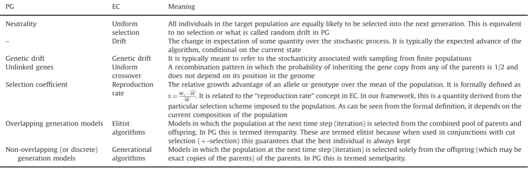
[image:8.595.43.563.82.249.2]

where Mt_{denotes the operator formed by composing M with itself} Table 1

A list of concepts in bothfields and their translation between thefields.

PG EC Meaning

Neutrality Uniform selection

All individuals in the target population are equally likely to be selected into the next generation. This is equivalent to no selection or what is called random drift in PG

– Drift The change in expectation of some quantity over the stochastic process. It is typically the expected advance of the algorithm, conditional on the current state

Genetic drift Genetic drift It is typically meant to refer to the stochasticity associated with sampling fromfinite populations Unlinked genes Uniform

crossover

A recombination pattern in which the probability of inheriting the gene copy from any of the parents is 1/2 and does not depend on its position in the genome

Selection coefficient Reproduction rate

The relative growth advantage of an allele or genotype over the mean of the population. It is formally defined as

s¼WiW

W . It is related to the“reproduction rate”concept in EC. In our framework, this is a quantity derived from the

particular selection scheme imposed to the population. As can be seen from the formal definition, it depends on the current composition of the population

Overlapping generation models Elitist algorithms

Models in which the population at the next time step (iteration) is selected from the combined pool of parents and offspring. In PG this is termed iteroparity. These are termed elitist because when used in conjunctions with cut selection (þ-selection) this guarantees that the best individual is always kept

Non-overlapping (or discrete) generation models

Generational algorithms

ttimes. We hold(M2)to be the defining characteristic of mutation operators.

To illustrate variation operators and their properties, we now discuss common mutation operators.

Uniform mutation: LetG¼

_Σ

1

Σ

2⋯

Σ

nwhere each

Σ

iis a

finite set of at least two elements. ForpA½0;1, uniform mutation is a random operator Mp:G-Gdefined as follows. For any string xAG, the result of applying the operator to x is another string MpðxÞ ¼ ðY1;…;YnÞ where each Yi is an independent random

variable de_fined for allyiA

Σ

i by

Pr Yi¼yi

¼

1p ifyi¼xi and p

j

_Σ

ij 1

otherwise: 8

< :

In many applications in evolutionary computation, uniform muta-tion is performed on bitstrings, that is

Σ

i¼ f0;1gfor alliAf1;…;ng. In this case, when p¼1=n, we refer to the operator asstandard mutation, and denote it M1=n. It should be noted that this operator

satisfies properties(V1) and (M1). Moreover, as long as 0opo1, it also satisfies(M2)(seeLemma 2inAppendix A).

Single-point mutation: LetG¼

_Σ

1

Σ

2⋯

Σ

nwhere each

Σ

i is afinite set of at least two elements. Single-point mutation is a random operator Msp:G-G that acts as follows. For any string xAG, the result of applying the operator to x is another string MspðxÞ ¼ ðY1;k;Y2;k;…;Yn;kÞwhere kUnifð1;nÞ and eachYi;k is a dependent random variable de_fined for allyiA

Σ

iwith

Pr Yi_;k¼yi

¼

1 ifiak; yi¼xi and 1

j

_Σ

ij 1

ifi¼k; yiA

Σ

i⧹fxig and

0 otherwise: 8

> > > < > > > :

Single-point mutation satisfies properties(V1), (M1), and (M2)

(Appendix A,Lemma 3).

4.2.2. Recombination operators

The role of recombination is to generate variation at the genotypic level, by shuffling information contained in the existing genotypes. In order to define recombination we require that the elements of G are ordered Cartesian products of sets: gA

Σ

1

Σ

2⋯

Σ

n, where

Σ

iis the set of available symbols at positioni, e.g. we do not require

Σ

i¼

Σ

jforiaj.

Let ½ denote the Iverson bracket, which denotes a 1 if the condition inside the bracket is true and 0 otherwise. We define the allele frequency of alleleaA

Σ

i in populationPat positionias

pPða;iÞ ¼ 1 P j j

X

gAP

½a4gi¼a:

Given these definitions, we define recombination operators as

R:Gk_-Gℓ_;

wherek;ℓAN. Here, R is a random operator that acts on aparent population of sizekto produce anoffspringpopulation of sizeℓ.

We require that a proper recombination operator RðPÞshould, in expectation, preserve allele frequencies from the population of parents. Formally, we require that

8iA½n; 8aA

Σ

i:E pRðPÞða;iÞ

h i

¼pPða;iÞ: ðR1Þ

Similar to mutation operators, we can describe recombination acting on both thepopulation leveland theindividual level. At the individual level, we define a recombination operator as a random m-ary operator R:Gm_-Gk_{, wherekAf1;2g, that produces one or} two offspring givenm41 parents. The recombination operator on individuals can then beliftedto the population level by concatena-tion and composiconcatena-tion with selecconcatena-tion, that is, given a populaconcatena-tionP

of sizek,

RðPÞ ¼ ððR○SÞðPÞÞi¼1…ℓ

where S:Gk_-Gm _{is a selection operator. Because the role of S in} this case is to select parents for R, we refer to the operation as parent selection.

If parent selection preserves uniform frequencies in expecta-tion, for example selectingmparents uniformly at random from P(t), then if property (R1) holds for an operator R, the allele frequencies in the offspring are preserved in expectation after parent selection and recombination (Appendix A,Lemma 4). If a recombination operator produces the two recombinant offspring, then it preserves allele frequencies exactly, not just in expectation. Moreover, if recombination is performed afinite number of times at the individual level to build up an intermediate population by concatenation, as long as the above properties hold, then the expected allele frequencies in the intermediate population are equal to the allele frequencies in the original population

(Appendix A,Lemma 5).

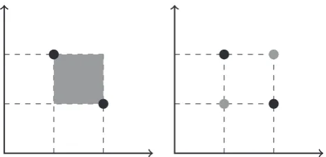
For commonly defined recombination operators, the result of RðPÞwill be in the convex hull ofP. However, our restriction on recombination operators excludes some recombination operators, such as geometric crossover on Manhattan spaces. In this example, genotypes are points in continuous space and recombination generates new individuals in the square convex hull (due to the Manhattan metric) between those two points. This does not fulfil our restriction for recombination, since it would not preserve the allele frequencies for the parent genotypes, and instead it con-stitutes a hybrid operator between recombination and mutation. A proper recombination operator would generate only the geno-types at the corners of the hypercube defined by the parent genotypes (Fig. 4).

Abstract frameworks for generalizing crossover have been proposed before Moraglio (2011). Our approach differs by not focussing on“natural”metrics of the genotype space, but instead focussing on the result of the application of recombination on elements of this space. We require the genotype space to be an ordered Cartesian product of sets (of alleles), and define recombi-nation as an operation that does not change the frequencies of these symbols on a population. It is in a sense more general than previous approaches, since it does not rely on external information about this space, such as the metric of the space, which may not be relevant for evolutionary processes (this fact has been previously articulated by Jones (1995) and Altenberg (1995)). In fact, our de_finition does not rely on the genotype being a metric space at all, even though one can always define a metric for Cartesian products of sets (the Hamming distance). However, this definition still respects the notion that the products of recombination are within the convex hull of the parental genotypes, for appropriately defined metrics. Indeed, if property(R1)holds for a recombination operator, then the resulting offspring lie in the convex hull of the parent population almost surely (Appendix A,Lemma 6).

Common recombination operators: We now instantiate common recombination operators and show that they satisfy properties of both variation and recombination operators.

One-point crossover: R1point:GG-G. This operator acts on pairs x;y of genotypes selected from the current population. A crossover point m_A½n1 is selected uniformly at random, and two new individualsz0andz″are produced, then one individual,z is uniformly selected at random, called offspring (children) where

z0i¼

xi ifirm; yi otherwise; (

z″i¼

yi ifirm; xi otherwise; (

crossover points are selected uniformly at random without repla-cement from½n1. Letm1;…;mk be a sorted list of these points andm0¼0;mkþ1¼n. Two new individualsz0andz″are produced as follows, then one individualzis uniformly selected at random, called offspring (children). For allisuch thatmjrirmjþ1

z0i¼

xi ifjmod 2¼0; yi otherwise; (

z″i¼

yi ifjmod 2¼0; xi otherwise; (

Note thatk-point crossover withk¼1 yields one-point crossover. Moreover,k-point crossover is a proper recombination operator in the sense that it preserves allele frequencies (Appendix A,

Lemma 7).

Uniform crossover: RUnif:GG-G≔ðg;g0Þ↦his defined as fol-lows. The allele at hi is inherited from gi with probability 1/2,

otherwise it is inherited fromg0_i for alliA½n. This operator also preserves allele frequencies and hence satisfies(R1)(Appendix A,

Lemma 7).

All crossover operators introduced here are uniformity-preserving and satisfy(V1)(Appendix A,Lemma 8).

4.2.3. Unbiased variation operators

The unbiased black-box model introduced byLehre and Witt

(2012), defines a general class of variation operators over the

genospace G¼ f0;1gn

(see also the extension inRowe and Vose

(2011) for other search spaces). Many variation operators on

bitstrings, such as bitwise mutation and uniform crossover, are unbiased variation operators. For any integerk, ak-ary unbiased variation operatoris any random operator V:Gk_{-G that for all} y;z;x1;…;xkAGand any permutation

σ

:½n-½nsatisfies PrðX¼y∣XVðx1;…;xkÞÞ ¼PrðY¼yz∣YVðx1z;…;xkzÞÞ; PrðX¼y∣XVðx1;…;xkÞÞ ¼PrðY¼

σ

ðyÞ∣YVð

σ

bðx1Þ;…;

σ

bðxkÞÞÞ;

where

σ

b is the permutation over G defined for all yAG by

σ

bðy1y2⋯ynÞ≔yσð1Þyσð2Þ…yσðnÞandmeans bitwise XOR between sequences. In the special case of unary variation (k¼1), the unbiased conditions imply that a genotype is mutated with equal probability into any other genotype at a given distance. This has been described as a desirable property of mutation operators (Droste and Wiesmann, 2000). Note that byLemma 1

with

σ

ðuÞ ¼x1yu, any k-ary unbiased variation operator satisfies(V1).

5. Instantiation of evolutionary models

We now show how common evolutionary models and algo-rithms can be instantiated in our framework, and which of these

fulfil common properties of our framework. We organize the following section based on the size of population they maintain (or more specifically on the amount of variability they maintain during the evolutionary process), since this seems to be the main factor that differentiates between results in bothfields.

In PG it has been found that the interplay between the influx of new mutation and the time they take to go tofixation (which is related to the strength of selection acting on the population) plays an important part in determining the variability present in the evolving population and hence, its evolutionary dynamics.

In EC these restrictions typically do not apply, since many schemes can be implemented that enforce either reduced or increased diversity in the population, which effectively decouple diversity in the population from mutation rate or population size. Thefield of evolutionary computation contains a large variety of evolutionary algorithms for optimizing a single objective func-tion, as well as variants for multiple objectives. In this paper, we focus on single-objective evolutionary algorithms, and defer the discussion of multi-objective variants to future work. We also include the so-called estimation-of-distribution algorithms

(Larrañaga and Lozano, 2002), a relatively new approach in EC

that adopts rather the distribution/sampling point of view than population/applying-operators one.

A common notation for evolutionary algorithms is the ð

_μ

þ;

_λ

_{Þ-notation (see Beyer and Schwefel, 2002), originally} devel-oped to classify evolutionary strategies, a type of evolutionary algorithm for continuous search spaces. In any generation t, a ð

_μ

þ;

_λ

_{ÞEA selects the best}

μ

_{individuals from the populationP(t).} These individuals are called the parents. The algorithm then generates

λ

offspringindividuals from the parents. The notation distinguishes between comma-selectionand plus-selection, which represent alternative ways to construct the population from which the new generation is sampled from. In að

_μ

;

λ

ÞEA, the selection operator is applied only to the

λ

offspring individuals. Such models are also called generational models or non-elitist models (see

Table 1). In að

μ

þ

λ

ÞEA, the next generation is selected from the

combined pool of both the

μ

parents and the

λ

offspring indivi-duals. This strategy–often referred to aselitism–ensures that the best individuals never die (seeTable 1).

In each generation of a (

μ

þ

λ

) EA,

λ

parents are being selected uniformly at random (Beyer and Schwefel, 2002). New offspring are being created by applying a mutation operator to these parents. Finally, cut selection chooses the best

μ

individuals among the

μ

þ

_λ

individuals, with ties being broken in favour of keeping offspring. This sequence of individuals replaces the current population.

Pðtþ1Þ ¼SCutðf;μÞPðtÞ [M1=n○SUnifðλÞðPðtÞÞ:

A further distinction is made by whether recombination operators are being used or not. If the algorithm does not use any kind of recombination operator, it is called a mutation-only EA, which many times is shortened to simply EA (even though the consensus is that all search heuristics inspired by natural evolution are EAs). If recombination is in use, it is considered a Genetic Algorithm(GA).

The (

μ

þ

λ

) EA extends to recombination as follows. We call the result a (

μ

þ

λ

) GA,Genetic Algorithm, as this term emphasizes the use of recombination in contrast to the term Evolutionary Algo-rithm. Recombination is typically applied to the set of selected parents. There is an additional parameter called crossover prob-ability pc, which determines the likelihood of two parents actually

being recombined. Formally, recombination creates

λ

pairs of parents, and for each pair it is decided independently whether crossover is being performed or not. With probability pc both

[image:10.595.51.287.55.169.2]

parents are crossed and one offspring is being returned for this pair. Otherwise, one of the two parents is returned uniformly at Fig. 4.Improper and proper geometric crossovers. In this example,Gis defined as

G¼RR. For two parental genotypesg1¼ ðx1;y1Þandg2¼ ðx2;y2Þcrossover could

defined either as the convex hull (under some metricd) of the two genotypes: Rðg1;g2Þ ¼Convdðg1;g2Þor as the union of the parental points and their position

wise permutations: Rðg1;r2Þ ¼ fg1;g2;ðx2;y1Þ;ðx1;y2Þg. Black circles represent

random. It is easy to see that (R1) still holds for crossover probabilities pco1 if it holds for pc¼1. The outcome of the

recombination operator is then mutated and fed into a cut selection operator as for the (

μ

þ

_λ

) EA.

The crossover operator may be k-point crossover or uniform crossover; we denote it by Rpc _{here to include the crossover} probability.

Pðtþ1Þ ¼SCutðf;μÞPðtÞ [ ðM1=n○Rpc○SUnifðλÞÞðPðtÞÞ:

Note that the (

μ

þ

λ

) EA emerges as a special case whenpc¼0 as

then no recombination is performed.

Several choices of

μ

and

λ

are of particular interest: the (1þ1) EA is arguably the simplest EA and among the best studied ones. The (

μ

þ1) EA was introduced for its mathematical simplicity and is a modification of theSteady State EA(Syswerda and Rawlins, 1991). In the same way, a (

μ

þ1) GA is also often called a Steady-Statealgorithm. In the following we will mention some of these special cases as we compare them to specific evolutionary regimes from PG.

5.1. Models of monomorphic populations

The simplest type of evolutionary model is when only one genotype is present in the population at any given time. This is true in PG only under certain assumptions on the influx of new mutations. However, this can be enforced by an evolutionary algorithm for parameter ranges (for example on the mutation rate) that can be outside this range.

SSWM regime: The Strong Selection Weak Mutation model applies when the population size, mutation rate and selection strength are such that the time between occurrence of new mutationsðtmut 1=N

μ

Þis long compared to the time offixation of a new mutation ðtfix logðNsÞ=sÞ (Gillespie, 1983) (notice another difficulty in translation between the two fields: here N is the population size, and

μ

is the mutation rate, while in the EC community,

μ

is the parent population size. For easier accessibility for both communities, we use the typical notation for each community). In this situation, the population is monomorphic (i. e. only one genotype present in the population) most of the time, and evolution occurs in “jumps” between different genotypes (when a new mutation fixes in the population). The relevant dynamics can then be characterized by this “jumping” process. This model is obtained as an approximation to a limit of many other models, such as the Wright–Fisher model. Moreover, this jumping process is also the approach to dynamics employed by adaptive dynamics (Dieckmann, 1997) and its connection to population genetics has been explained by Matessi and

Schneider (2009)andSchneider (2007).

This model can be instantiated in many different genotype spaces. Here, for illustrative purposes, we use Gk _{as genotype} space. In this case, the relevant mutation operator is, for example, M_μ. Recombination does not apply to this model since the population is always monomorphic (only one genotype in the population at all times). The typical selection operator is propor-tional selection, with some function w, typically some form of probability offixation. Because in this model the population size is one, this function will tend to choose preferentially individuals of higher values of the objective function (selection coefficient –

Table 1).

Evolution then proceeds by the successive application of these operators:

Pðtþ1Þ ¼SPropðw;1ÞðPðtÞ [MðPðtÞÞÞ:

(1þ1)EA: The (1þ1) Evolutionary Algorithm is arguably the simplest possible evolutionary algorithm and has been a very popular choice for theoretical research on the performance of

evolutionary algorithms. It represents a“bare-bones”evolutionary algorithm with a population of size 1. Because of this, no recombination is used. The (1þ1) EA mutates its current indivi-dual, and then survival selection picks the best of the offspring and the parent genotypes. Ties in this cut selection are broken towards favouring the offspring. The default mutation operator is bitwise mutation with mutation rate 1=n. It is formalized by

Pðtþ1Þ ¼SCutðf;1ÞPðtÞ [M1=nðPðtÞÞ:

Simulated annealing: Although not usually considered an evolu-tionary algorithm, simulated annealing also maintains a popula-tion of one individual, which is mutated. Then, one individual is chosen to constitute the next generation with a probability that depends on their relative value of the objective function. Simu-lated annealing makes use of replacement selection explicitly. The model is described by

Pðtþ1Þ ¼SRep;hðPðtÞ [MðPðtÞÞÞ

withhde_fined as

hð

_Δ

Þ ¼ 1 if

Δ

40 eγtΔ otherwise (

where

γ

_tAR is a parameter controlling the degree to which deleterious mutations are accepted. Typically,

γ

t is a function of

time and represents the cooling schedule of the algorithm, making it harder to accept worse solutions as time goes on.

Atfirst glance, the (1þ1) EA and the SSWM regime seem to share some similarities, as they both evolve just one genotype. It is reassuring that these similarities are captured in our framework. There is an obvious structural similarity between the two models, with the only difference being that the (1þ1) EA uses cut selection SCutð;Þwhile the SSWM model uses SPropð Þ as selection operator. The consequence of this difference is that in the SSWM regime some mutations may notfix even if they are beneficial. This, of course depends on the choice of the probability offixation used in the SPropð Þ, which, in some circumstances could be justified to be close to cut selection (choosing the best among the current genotype and its mutated version).

SSWM can be regarded in some sense as a slower version of the (1þ1) EA, as in the former some beneficial mutations may be rejected. On the other hand, in the SSWM regime the average “jump” will be larger than in the (1þ1) EA. A more important difference is that SSWM may accept detrimental steps, depending on the form of probability offixation used, whereas the (1þ1) EA will not. The behaviour of SSWM in that respect resembles that of simulated annealing (Kirkpatrick et al., 1983). However, depending on the choice of the probability offixation in SSWM, SSWM and (1þ1) EA may follow similar trajectories and show similar dynamics.

It is interesting that both SSWM and (1þ1) EA can also be cast in terms of replacement selection operators. For SSWM, one would choosehas the probability of_fixation of a new genotype, given its objective function value, and for (1þ1) EA one would choosehð

_Δ

Þ to be 1 for

Δ

Z0 and 0 otherwise.

Because there is a substantial body of work in all three models, we expect a translation of results to prove very fruitful for both

fields. Furthermore, the consequences of the (small) difference in selection operators will also be analyzed.

5.2. Models of polymorphic populations with“slow”dynamics