Applied Combinatorics

(1)

Applied

Combinatorics

2017 Edition

Keller

Trotter

(2)

(3)

(4)

Applied Combinatorics

Mitchel T. Keller

Washington and Lee University

Lexington, Virginia

William T. Trotter

Georgia Institute of Technology

Atlanta, Georgia

(5)

Edition: 2017 Edition

Website:http://rellek.net/appcomb/

(6)

(7)

Summary of Contents

About the Authors ix

Acknowledgements xi

Preface xiii

Preface to 2017 Edition xv

Preface to 2016 Edition xvii

Prologue 1

1 An Introduction to Combinatorics 3

2 Strings, Sets, and Binomial Coefficients 17

3 Induction 39

4 Combinatorial Basics 59

5 Graph Theory 69

6 Partially Ordered Sets 113

7 Inclusion-Exclusion 141

8 Generating Functions 157

9 Recurrence Equations 183

10 Probability 213

11 Applying Probability to Combinatorics 229

(8)

13 Network Flows 259

14 Combinatorial Applications of Network Flows 279

15 Pólya’s Enumeration Theorem 291

16 The Many Faces of Combinatorics 315

A Epilogue 331

B Background Material for Combinatorics 333

C List of Notation 361

(9)

About the Authors

About William T. Trotter

William T. Trotter is a Professor in the School of Mathematics at Georgia Tech. He was ﬁrst exposed to combinatorial mathematics through the 1971 Bowdoin Combi-natorics Conference which featured an array of superstars of that era, including Gian Carlo Rota, Paul Erdős, Marshall Hall, Herb Ryzer, Herb Wilf, William Tutte, Ron Gra-ham, Daniel Kleitman and Ray Fulkerson. Since that time, he has published more than 120 research papers on graph theory, discrete geometry, Ramsey theory, and ex-tremal combinatorics. Perhaps his best known work is in the area of combinatorics and partially ordered sets, and his 1992 research monograph on this topic has been very inﬂuential. (He takes some pride in the fact that this monograph is still in print and copies are being sold in 2016.) He has more than 70 co-authors, but considers his extensive joint work with Graham Brightwell, Stefan Felsner, Peter Fishburn, Hal Kier-stead and Endre Szemerèdi as representing his best work. His career includes invited presentations at more than 50 international conferences and more than 30 meetings of professional societies. He was the founding editor of theSIAM Journal on Discrete Math-ematicsand has served on the Editorial Board ofOrdersince the journal was launched in 1984, and his service includes an eight year stint as Editor-in-Chief. Currently, he serves on the editorial boards of three other journals in combinatorial mathematics.

Still he has his quirks. First, he insists on being called “Tom”, as Thomas is his middle name, while continuing to sign as William T. Trotter. Second, he has invested time and energy serving five terms as department/school chair, one at Georgia Tech, two at Arizona State University and two at the University of South Carolina. In addition, he has served as a Vice Provost and as an Assistant Dean. Third, he is fascinated by computer operating systems and is always installing new ones. In one particular week, he put eleven different flavors of Linux on the same machine, interspersed with four complete installs of Windows 7. Incidentally, the entire process started and ended with Windows 7. Fourth, he likes to hit golf balls, not play golf, just hit balls. Without these diversions, he might even have had enough time to settle the Riemann hypothesis.

(10)

About Mitchel T. Keller

Mitchel T. Keller is a super-achiever (this description is written by WTT) extraordi-naire from North Dakota. As a graduate student at Georgia Tech, he won a lengthy list of honors and awards, including a VIGRE Graduate Fellowship, an IMPACT Scholar-ship, a John R. Festa Fellowship and the 2009 Price Research Award. Mitch is a natural leader and was elected President (and Vice President) of the Georgia Tech Graduate Student Government Association, roles in which he served with distinction. Indeed, after completing his terms, his student colleagues voted to establish a continuing award for distinguished leadership, to be named the Mitchel T. Keller award, with Mitch as the ﬁrst recipient. Very few graduate students win awards in the ﬁrst place, but Mitch is the only one I know who has an awardnamedafter them.

Mitch is also a gifted teacher of mathematics, receiving the prestigious Georgia Tech 2008 Outstanding Teacher Award, a campus-wide competition. He is quick to exper-iment with the latest approaches to teaching mathematics, adopting what works for him while reﬁning and polishing things along the way. He really understands the lit-erature behind active learning and the principles of engaging students in the learning process. Mitch has even taught his more senior (some say ancient) co-author a thing or two and got him to try personal response systems in a large calculus section.

Mitch is oﬀ to a fast start in his own research career, and is already an expert in the subject of linear discrepancy. Mitch has also made substantive contributions to a topic known as Stanley depth, which is right at the boundary of combinatorial mathematics and algebraic combinatorics.

After ﬁnishing his Ph.D., Mitch received another signal honor, a Marshall Sherﬁeld Postdoctoral Fellowship and spent two years at the London School of Economics. He is presently an Assistant Professor of Mathematics at Washington and Lee University, and a few years down the road, he’ll probably be president of something.

(11)

Acknowledgements

We are grateful to our colleagues Alan Diaz, Thang Le, Noah Streib, Prasad Tetali and Carl Yerger, who have taught Applied Combinatorics from preliminary versions and have given valuable feedback. As this text is freely available on the internet, we wel-come comments, criticisms, suggestions and corrections from anyone who takes a look at our work.

(12)

(13)

Preface

At Georgia Tech, MATH 3012: Applied Combinatorics, is a junior-level course tar-geted primarily at students pursuing the B.S. in Computer Science. The purpose of the course is to give students a broad exposure to combinatorial mathematics, using applications to emphasize fundamental concepts and techniques. Applied Combina-torics is also required of students seeking the B.S. in Mathematics, and it is one of two discrete mathematics courses that computer engineering students may select to fulﬁll a breadth requirement. The course will also often contain a selection of other engi-neering and science majors who are interested in learning more mathematics. As a consequence, in a typical semester, some 250 Georgia Tech students are enrolled in Applied Combinatorics. Students enrolled in Applied Combinatorics at Georgia Tech have already completed the three semester calculus sequence—with many students bypassing one or more of the these courses on the basis of advanced placement scores. Also, the students will know some linear algebra and can at least have a reasonable discussion about vector spaces, bases and dimension.

Our approach to the course is to show students the beauty of combinatorics and how combinatorial problems naturally arise in many settings, particularly in computer science. While proofs are periodically presented in class, the course is not intended to teach students how to write proofs; there are other required courses in our curriculum that meet this need. Students may occasionally be asked to prove small facts, but these arguments are closer to the kind we expect from students in second or third semester calculus as contrasted with proofs we expect from a mathematics major in an upper-division course. Regardless, we cut very few corners, and our text can readily be used by instructors who elect to be even more rigorous in their approach.

(14)

applications, including algorithms. We do not get deeply into the details of what it means for an algorithm to be “eﬃcient”, but we do include an informal discussion of the basic principles of complexity, intended to prepare students in computer science, engineering and applied mathematics for subsequent coursework.

The materials included in this book have evolved over time. Early versions of a few chapters date from 2004, but the pace quickened in 2006 when the authors team taught a large section of Applied Combinatorics. In the last ﬁve years, existing chapters have been updated and expanded, while new chapters have been added. As matters now stand, our book includes more material than we can cover in a single semester. We feel that the topics of Chapters 1–9 plus Chapters 12, 13 and 14 are the core of a one semester course in Applied Combinatorics. Additional topics can then be selected from the remaining chapters based on the interests of the instructor and students.

(15)

Preface to 2017 Edition

Because I (mtk) didn’t have the chance to teach from this book during the 2016–2017 academic year, there were few opportunities to examine some of the areas where im-provements are due in the text. That said, some changes suggested in thePreface to 2016 Editiondid come to fruition in this edition. In particular, the numbering of many things inChapter 8 will not match the 2016 Edition in a number of places because of the addition ofExample 8.7to address the coeﬃcients on1/(1−x)n in a way that doesn’t require calculus. There is also one new exercise inChapter 8, which has been placed at the end to retain consistency of numbering. Other than correcting errors, there have been no changes to the exercises, so faculty members teaching from the text may continue to assign the same exercise numbers with conﬁdence that they are the same exercises they have been in the past.

The other notable update in this edition is the addition of a number of SageMathCells toChapter 8 (including in the exercises), Section 9.6, and the Discussion that ends Chapter 9. The practice of vaguely referring readers to a generic computer algebra system but not providing any advice on how to use it had always been unsatisfying. I know there are places where further reﬁnement is in order, but this edition starts a more coherent approach toward using technology for some of the unpleasant algebraic aspects of the text. Readers can edit the content of the SageMathCells in the body of the text in order to use them to tackle other problems, and those in the exercises are there for convenience more than anything and include only a bare skeleton of what might be useful for the exercise. Since SageMath is open source and can be run for free on CoCalc, this approach seems greatly preferable to targeting a commercial CAS.For those, like me, who are coming to SageMath with experience using a commercial CAS, SageMath does not do implied multiplication in input very well. When a result comes up that seems strange, my ﬁrst step is always to make sure that I’m not missing a*

in my code.

Of course, even in a text that’s been in use for over a decade, there are typos. A num-ber of small issues were resolved in this edition. The errata pagehttp://www.rellek.net/ appcomb/errata/lists the dozen mistakes corrected in this edition. Undoubtedly, there are other mistakes waiting to be found, and we welcome reports from readers. (Pull requests on GitHub are also welcome!)

(16)

alongside our text, contributions of code snippets that would be worth including are also welcomed.

(17)

Preface to 2016 Edition

In April 2016, the American Institute of Mathematics hosted a weeklong workshop in San Jose to introduce authors of open textbooks togitand Robert A. Beezer’s Math-Book xml authoring language designed to seamlessly produce html, LA_{TEX, and other} formats from a common xml source file. I (mtk) attended and eagerly began the con-version of existing LA_{TEX source for this now decade-old project into MathBook xml.} David Farmer deserves an enormous amount of credit for automating much of the process through a finely-tuned script, but the code produced still required a good deal of cleanup. This edition, the first not labeled “preliminary”, will hopefully become the first of many annual editions ofApplied Combinatoricsreleased under an open source license.

The main effort in producing this 2016 edition was to successfully convert to Math-Book xml. Along the way, I attempted to correct all typographical errors we had noted in the past. There are undoubtedly more errors (typographical or otherwise) that will be corrected in future years, so please contact us via email if you spot any. The text now has an index, which may prove more helpful than searching PDF files when looking for the most essential locations of some common terms. Since MathBook xml makes it easy, we now also have a list of notation. Instructors will likely be glad to know that there were no changes to the exercises, so lists of assigned exercises from past years remain completely valid.¹ The only significant changes to the body of the text was to convert wtt’s code snippets from C to Python/SageMath. This has allowed us to em-bed interactive SageMath cells that readers who use the html version of the text can run and edit. We’ve only scratched the surface with this powerful feature of MathBook xml, so look for more SageMath additions in future years.

The conversion to MathBook xml allows us to make a wider variety of formats avail-able:

• html: With responsive design using css, we feel that the text now looks beautiful on personal computers, tablets, and even mobile phones. No longer will students be frantically resizing a PDF on their phone in order to try to read a passage from the text. The “knowls” oﬀered in html also allow references to images, tables, and

¹There are two exceptions to this. The ﬁrst is thatExercise 8.8.7has been modiﬁed to make the computations involved cleaner. We have preserved the exercise that was previously in this position asExercise 8.8.27

(18)

even theorems from other pages (or even a distance away on the same page) to provide a copy of the image/table/theorem right there, and another click/tap makes it disappear.

• pdf: Not much is changed here from previous years, other than the pdf is pro-duced from the LA_{TEX that MathBook xml generates, and so numbering and order} is consistent with the html version.

• Print: Campus bookstores have frequently produced printed versions of the text from the pdf provided online, but we have not previously been able to provide a printed, bound version for purchase. With the 2016 edition, we are pleased to launch a print version available through a number of online purchase channels. Campus bookstores may also acquire the book through wholesale channels for sale directly to students. Because of the CreativeCommons license under which the text is released, campuses retain the option of selling their own printed ver-sion of the text for students, although this is likely only ﬁnancially advantageous to students if only a few chapters of the text are being used.

We have some ideas for what might be updated for the 2017 Edition (e.g.,Chapter 4 needs to be expanded both in the body and the exercises,Chapter 8would beneﬁt from integration of SageMath to assist with generating function computations, and Chap-ter 16is still not really ﬁnished). However, we would love to hear from those of you who are using the text, too. Are there additional topics you’d like to see added? Chap-ters in need of more exercises? Topics whose exposition could be improved? Please reach out to us via email, and we’ll consider your suggestions.

(19)

11.1 A First Taste of Ramsey Theory . . . 229 11.2 Small Ramsey Numbers . . . 230 11.3 Estimating Ramsey Numbers . . . 231 11.4 Applying Probability to Ramsey Theory . . . 232 11.5 Ramsey’s Theorem . . . 233 11.6 The Probabilistic Method . . . 234 11.7 Discussion . . . 235 11.8 Exercises . . . 236

12 Graph Algorithms 239

12.1 Minimum Weight Spanning Trees . . . 239 12.2 Digraphs . . . 245 12.3 Dĳkstra’s Algorithm for Shortest Paths . . . 245 12.4 Historical Notes . . . 252 12.5 Exercises . . . 253

13 Network Flows 259

13.1 Basic Notation and Terminology . . . 259 13.2 Flows and Cuts . . . 261 13.3 Augmenting Paths . . . 263 13.4 The Ford-Fulkerson Labeling Algorithm . . . 267 13.5 A Concrete Example . . . 269 13.6 Integer Solutions of Linear Programming Problems . . . 273 13.7 Exercises . . . 274

14 Combinatorial Applications of Network Flows 279

14.1 Introduction . . . 279 14.2 Matchings in Bipartite Graphs . . . 280 14.3 Chain partitioning . . . 284 14.4 Exercises . . . 287

15 Pólya’s Enumeration Theorem 291

(23)

Contents

16 The Many Faces of Combinatorics 315

16.1 On-line algorithms . . . 315 16.2 Extremal Set Theory . . . 318 16.3 Markov Chains . . . 320 16.4 The Stable Matching Theorem . . . 322 16.5 Zero–One Matrices . . . 323 16.6 Arithmetic Combinatorics . . . 325 16.7 The Lovász Local Lemma . . . 326 16.8 Applying the Local Lemma . . . 328

A Epilogue 331

B Background Material for Combinatorics 333

B.1 Introduction . . . 333 B.2 Intersections and Unions . . . 334 B.3 Cartesian Products . . . 337 B.4 Binary Relations and Functions . . . 337 B.5 Finite Sets . . . 339 B.6 Notation from Set Theory and Logic . . . 340 B.7 Formal Development of Number Systems . . . 341 B.8 Multiplication as a Binary Operation . . . 344 B.9 Exponentiation . . . 345 B.10 Partial Orders and Total Orders . . . 346 B.11 A Total Order on Natural Numbers . . . 347 B.12 Notation for Natural Numbers . . . 348 B.13 Equivalence Relations . . . 350 B.14 The Integers as Equivalence Classes of Ordered Pairs . . . 350 B.15 Properties of the Integers . . . 351 B.16 Obtaining the Rationals from the Integers . . . 353 B.17 Obtaining the Reals from the Rationals . . . 355 B.18 Obtaining the Complex Numbers from the Reals . . . 356 B.19 The Zermelo-Fraenkel Axioms of Set Theory . . . 358

C List of Notation 361

(24)

(25)

Prologue

A unique feature of this book is a recurring cast of characters: Alice, Bob, Carlos, Dave, Xing, Yolanda and Zori. They are undergraduate students at Georgia Tech, they’re taking an 8:05am section of Math 3012: Applied Combinatorics, and they frequently go for coﬀee at the Clough Undergraduate Learning Center immediately after the class is over. They’ve become friends of sorts and you may ﬁnd their conversations about Applied Combinatorics of interest, as they will may reveal subtleties behind topics currently being studied, reinforce connections with previously studied material or set the table for topics which will come later. Sometimes, these conversations will set aside in a clearly markedDiscussionsection, but they will also be sprinkled as brief remarks throughout the text.

In time, you will get to know these characters and will sense that, for example, when Dave comments on a topic, it will represent a perspective that Zori is unlikely to share. Some comments are right on target while others are “out in left ﬁeld.” Some may even be humorous, at least we hope this is the case. Regardless, our goal is not to entertain— although that is not all that bad a side beneﬁt. Instead, we intend that our informal approach adds to the instructional value of our text.

Now it is time to meet our characters:

Aliceis a computer engineering major from Philadelphia. She is ambitious, smart and intense. Alice is quick to come to conclusions, most of which are right. On occa-sion, Alice is not kind to Bob.

Bobis a management major from Omaha. He is a hard working and conscientious. Bob doesn’t always keep pace with his friends, but anything he understands, he owns, and in the end, he gets almost everything. On the other hand, Bob has never quite understood why Alice is short with him at times.

Carlosis a really, really smart physics major from San Antonio. He has three older brothers and two sisters, one older, one younger. His high school background wasn’t all that great, but Carlos is clearly a special student at Georgia Tech. He absorbs new concepts at lightning speed and sees through to the heart of almost every topic. He thinks carefully before he says something and is admirably polite.

(26)

Xingis a computer science major from New York. Xing’s parents immigrated from Beĳing, and he was strongly supported and encouraged in his high school studies. Xing is detail oriented and not afraid to work hard.

Yolandais a double major (computer science and chemistry) from Cumming, a small town just north of Atlanta. Yolanda is the ﬁrst in her extended family to go to a college or university. She is smart and absorbs knowledge like a sponge. It’s all new to her and her horizons are raised day by day.

(27)

CHAPTER

1

An Introduction to Combinatorics

As we hope you will sense right from the beginning, we believe that combinatorial mathematics is one of the most fascinating and captivating subjects on the planet. Combinatorics isveryconcrete and has a wide range of applications, but it also has an intellectually appealing theoretical side. Our goal is to give you a taste of both. In order to begin, we want to develop, through a series of examples, a feeling for what types of problems combinatorics addresses.

1.1 Introduction

There are three principal themes to our course:

Discrete Structures Graphs, digraphs, networks, designs, posets, strings, patterns, distributions, coverings, and partitions.

Enumeration Permutations, combinations, inclusion/exclusion, generating functions, recurrence relations, and Pólya counting.

Algorithms and Optimization Sorting, eulerian circuits, hamiltonian cycles, planarity testing, graph coloring, spanning trees, shortest paths, network ﬂows, bipartite matchings, and chain partitions.

(28)

1.2 Enumeration

Many basic problems in combinatorics involve counting the number of distributions of objects into cells—where we may or may not be able to distinguish between the objects and the same for the cells. Also, the cells may be arranged in patterns. Here are concrete examples.

Amanda has three children: Dawn, Keesha and Seth.

1. Amanda has ten one dollar bills and decides to give the full amount to her chil-dren. How many ways can she do this? For example, one way she might dis-tribute the funds is to give Dawn and Keesha four dollars each with Seth receiv-ing the balance—two dollars. Another way is to give the entire amount to Keesha, an option that probably won’t make Dawn and Seth very happy. Note that hid-den within this question is the assumption that Amanda does not distinguish the individual dollar bills, say by carefully examining their serial numbers. Instead, we intend that she need only decide theamounteach of the three children is to receive.

2. The amounts of money distributed to the three children form a sequence which if written in non-increasing order has the form: a1,a2,a3witha1 ≥ a2 ≥ a3and

a1+a2+a3 10. How many such sequences are there?

3. Suppose Amanda decides to give each child at least one dollar. How does this change the answers to the ﬁrst two questions?

4. Now suppose that Amanda has ten books, in fact the top 10 books from the New York Times best-seller list, and decides to give them to her children. How many ways can she do this? Again, we note that there is a hidden assumption—the ten books are all diﬀerent.

5. Suppose the ten books are labeledB1,B2, . . . ,B10. The sets of books given to the

three children are pairwise disjoint and their union is {B1,B2, . . . ,B10}. How

many diﬀerent sets of the form{S1,S2,S3}whereS1,S2andS3are pairwise

dis-joint andS1∪S2∪S3 {B1,B2, . . . ,B10}?

6. Suppose Amanda decides to give each child at least one book. How does this change the answers to the preceding two questions?

(29)

1.3 Combinatorics and Graph Theory

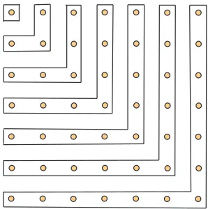
A circular necklace with a total of six beads will be assembled using beads of three different colors. InFigure 1.1, we show four such necklaces—however, note that the first three are actually thesamenecklace. Each has three red beads, two blues and one green. On the other hand, the fourth necklace has the same number of beads of each color but it is adifferentnecklace.

Figure 1.1:Necklaces made with three colors

1. How many diﬀerent necklaces of six beads can be formed using three reds, two blues and one green?

2. How many diﬀerent necklaces of six beads can be formed using red, blue and green beads (not all colors have to be used)?

3. How many diﬀerent necklaces of six beads can be formed using red, blue and green beads if all three colors have to be used?

4. How would we possibly answer these questions for necklaces of six thousand beads made with beads from three thousand diﬀerent colors? What special soft-ware would be required to ﬁnd the exact answer and how long would the com-putation take?

1.3 Combinatorics and Graph Theory

AgraphGconsists of avertexsetVand a collectionEof2-element subsets ofV.

Ele-ments ofEare callededges. In our course, we will (almost always) use the convention

thatV{1,2,3, . . . ,n}for some positive integern. With this convention, graphs can

be describedpreciselywith a text ﬁle:

1. The ﬁrst line of the ﬁle contains a single integern, the number of vertices in the graph.

(30)

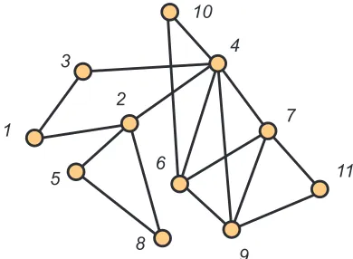
We illustrate this convention inFigure 1.2with a text ﬁle and the diagram for the graphGit deﬁnes.

graph1.txt 9

6 2 1 5 1 7 6 8 9 1 4 3 5 7 1 3 5 9 7 9

1

5 3

6

4 2

7

8 9

Figure 1.2:A graph defined by data

Much of the notation and terminology for graphs is quite natural. See if you can make sense out of the following statements which apply to the graphGdeﬁned above:

1. Ghas9vertices and10edges.

2. {2,6}is an edge.

3. Vertices5and9are adjacent.

4. {5,4}is not an edge.

5. Vertices3and7are not adjacent.

6. P(4,3,1,7,9,5)is a path of length5from vertex4to vertex5.

7. C(5,9,7,1)is cycle of length4.

8. Gis disconnected and has two components. One of the components has vertex set{2,6,8}.

9. {1,5,7}is a triangle.

10. {1,7,5,9}is a clique of size4.

(31)

1.3 Combinatorics and Graph Theory

Equipped only with this little bit of background material, we are already able to pose a number of interesting and challenging problems.

Example 1.3. Consider the graphGshown inFigure 1.4.

1

5 3

6 4

2 7

8 9

10 11

12

13 14

15

16

17 18

19 20

21

22 23

24

Figure 1.4:A connected graph

1. What is the largestkfor whichGhas a path of lengthk?

2. What is the largestkfor whichGhas a cycle of lengthk?

3. What is the largestkfor whichGhas a clique of sizek?

4. What is the largestkfor whichGhas an independent set of sizek?

5. What is the shortest path from vertex7to vertex6?

Suppose we gave the class a text data ﬁle for a graph on1500vertices and asked whether the graph contains a cycle of length at least500. Raoul says yes and Carla says no. How do we decide who is right?

Suppose instead we asked whether the graph has a clique of size500. Helene says that she doesn’t think so, but isn’t certain. Is it reasonable that her classmates insist that she make up her mind, one way or the other? Is determining whether this graph has a clique of size500harder, easier or more or less the same as determining whether it has a cycle of size500.

(32)

Example 1.5. InFigure 1.6, we show the location of some radio stations in the plane, together with a scale indicating a distance of200miles. Radio stations that are closer than200miles apart must broadcast on diﬀerent frequencies to avoid interference.

200 miles

1

3 4

6 5

2

4 5

1

3

4 6

5 1

4

6 1 2

4

6 5

3 ₆

5

Figure 1.6:Radio Stations

We’ve shown that6diﬀerent frequencies are enough. Can you do better?

Can you find4stations each of which is within200miles of the other3? Can you find8stations each of is more than200miles away from the other7? Is there a natural way to define a graph associated with this problem?

Example 1.7. How big must an applied combinatorics class be so that there are either

(a) six students with each pair having taken at least one other class together, or (b) six students with each pair together in a class for the ﬁrst time. Is this really a hard problem or can we ﬁgure it out in just a few minutes, scribbling on a napkin?

1.4 Combinatorics and Number Theory

Broadly, number theory concerns itself with the properties of the positive integers. G.H. Hardy was a brilliant British mathematician who lived through both World Wars and conducted a large deal of number-theoretic research. He was also a paciﬁst who was happy that, from his perspective, his research was not “useful”. He wrote in his 1940 essayA Mathematician’s Apology“[n]o one has yet discovered any warlike purpose to be served by the theory of numbers or relativity, and it seems very unlikely that anyone will do so for many years.”¹ Little did he know, the purest mathematical ideas

(33)

1.4 Combinatorics and Number Theory

of number theory would soon become indispensable for the cryptographic techniques that kept communications secure. Our subject here is not number theory, but we will see a few times where combinatorial techniques are of use in number theory.

Example 1.8. Form a sequence of positive integers using the following rules. Start with

a positive integern >1. Ifnis odd, then the next number is3n+1. Ifnis even, then the next number isn/2. Halt if you ever reach1. For example, if we start with28, the sequence is

28,14,7,22,11,34,17,52,26,13,40,20,10,5,16,8,4,2,1.

Now suppose you start with19. Then the ﬁrst few terms are

19,58,29,88,44,22.

But now we note that the integer22appears in the ﬁrst sequence, so the two sequences will agree from this point on. Sequences formed by this rule are calledCollatz se-quences.

Pick a number somewhere between100and200and write down the sequence you get. Regardless of your choice, you will eventually halt with a1. However, is there some positive integern(possibly quite large) so that if you start fromn, you will never reach1?

Example 1.9. Students in middle school are taught to add fractions by ﬁnding least

common multiples. For example, the least common multiple of15and12is60, so:

2 15+

7 12

8 60+

35 60

43 60.

How hard is it to ﬁnd the least common multiple of two integers?

It’s really easy if you can factor them into primes. For example, consider the problem of ﬁnding the least common multiple of351785000and316752027900if you just happen to know that

35178500023×54×7×19×232 and

31675202790022×3×52×73×11×234.

Then the least common multiple is

30091442650500023×3×54×73×11×19×234.

So to ﬁnd the least common multiple of two numbers, we just have to factor them into primes. That doesn’t sound too hard. For starters, can you factor1961? OK, how about1348433? Now for a real challenge. Suppose you are told that the integer

(34)

2043138898236817075547572153799

is the product of two primesaandb. Can you ﬁnd them?

What if factoring is hard? Can you ﬁnd the least common multiple of two relatively large integers, say each with about500digits, by another method? How should middle school students be taught to add fractions?

As an aside, we note that most calculators can’t add or multiply two20digits num-bers, much less two numbers with more than500digits. But it is relatively straight-forward to write a computer program that will do the job for us. Also, there are some powerful mathematical software tools available. Two very well known commercial ex-amples areMaple® andMathematica®. In this text, we will from time to time, make use of the open source computer algebra systemSageMath. We will sometimes embed interactive SageMath cells in the text, but you can also use SageMath for free online via theSageMath Cloud. For example, the SageMath cell below will produce the fac-torization shown above.

factor (300914426505000)

2^3 * 3 * 5^4 * 7^3 * 11 * 19 * 23^4

If you’re reading this text in a web browser, go ahead and change the integer in the SageMath cell above to some other, perhaps larger, integer and click the button again to get the prime factorization of your new integer.

Now here’s how we made up the challenge problem. First, we found a site on the web that lists large primes and found these two values:

a2425967623052370772757633156976982469681 and

b22953686867719691230002707821868552601124472329079.

The SageMath code below calculatesa×b, and returns the result instantly.

a = 2425967623052370772757633156976982469681

b = 22953686867719691230002707821868552601124472329079 a* b

On the other hand, if you ask SageMath to factorc, as in the cell below, you’ll likely be waiting a long time. If you get a response in more than a couple of minutes, please email us so that we can update the text with larger primesaandb!

(35)

1.5 Combinatorics and Geometry

Questions arising in number theory can also have an enumerative ﬂair, as the fol-lowing example shows.

Example 1.10. InFigure 1.11, we show the integer partitions of8.

8 distinct parts

7+1 distinct parts, odd parts

6+2 distinct parts

6+1+1

5+3 distinct parts, odd parts

5+2+1 distinct parts

5+1+1+1 odd parts

4+4

4+3+1 distinct parts

4+2+2

4+2+1+1

4+1+1+1+1

3+3+2

3+3+1+1 odd parts

3+2+2+1

3+2+1+1+1

3+1+1+1+1+1 odd parts

2+2+2+2

2+2+2+1+1

2+2+1+1+1+1

2+1+1+1+1+1+1

1+1+1+1+1+1+1+1 odd parts

Figure 1.11:The partitions of8, noting those into distinct parts and those into odd

parts.

There are22partitions altogether, and as noted, exactly6of them are partitions of8 into odd parts. Also, exactly6of them are partitions of8into distinct parts.

What would be your reaction if we asked you to ﬁnd the number of integer partitions of25892? Do you think that the number of partitions of25892into odd parts equals the number of partitions of25892into distinct parts? Is there a way to answer this question

withoutactually calculating the number of partitions of each type?

1.5 Combinatorics and Geometry

(36)

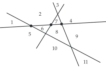
Example 1.12. InFigure 1.13, we show a family of4lines in the plane. Each pair of lines intersects and no point in the plane belongs to more than two lines. These lines determine11regions.

1

2

3

4 6

7 8

9

10 5

[image:36.545.183.407.128.268.2]

11

Figure 1.13:Lines and regions

Under these same restrictions, how many regions would a family of8947lines de-termine? Can diﬀerent arrangements of lines determine diﬀerent numbers of regions?

Example 1.14. Mandy says she has found a set of882points in the plane that determine

exactly752lines. Tobias disputes her claim. Who is right?

Example 1.15. There are many diﬀerent ways to draw a graph in the plane. Some

drawings may have crossing edges while others don’t. But sometimes, crossing edges must appear in any drawing. Consider the graphGshown inFigure 1.16.

1

2

3

4

5

6

7

8

9

10

[image:36.545.205.387.412.541.2]

(37)

1.6 Combinatorics and Optimization

Can you redrawGwithout crossing edges?

Suppose Sam and Deborah were given a homework problem asking whether a par-ticular graph on2843952 vertices and 9748032edges could be drawn without edge crossings. Deborah just looked at the number of vertices and the number of edges and said that the answer is “no.” Sam questions how she can be so certain—without look-ing more closely at the structure of the graph. Is there a way for Deborah to justify her deﬁnitive response?

1.6 Combinatorics and Optimization

You likely have already been introduced to optimization problems, as calculus students around the world are familiar with the plight of farmers trying to fence the largest area of land given a certain amount of fence or people needing to cross rivers down-stream from their current location who must decide where they should cross based on the speed at which they can run and swim. However, these problems are inher-ently continuous. In theory, you can cross the river at any point you want, even if it were irrational. (OK, so not exactly irrational, but a good decimal approximation.) In this course, we will examine a few optimization problems that are not continuous, as only integer values for the variables will make sense. It turns out that many of these problems are very hard to solve in general.

Example 1.17. InFigure 1.18, we use letters for the labels on the vertices to help

dis-tinguish visually from the integer weights on the edges.

11

17

4 2 16

13 12

9

3 7

27 10

32

19 14 5 18

8 28

A

B C

D E

F

G

H J

[image:37.545.151.348.370.540.2]

K

(38)

Suppose the vertices are cities, the edges are highways and the weights on the edges representdistance.

1. What is the shortest path from vertexEto vertexB?

2. Suppose Ariel is a salesperson whose home base is cityA. In what order should Ariel visit the other cities so that she goes through each of them at least once and returns home at the end—while keeping the total distance traveled to a min-imum? Can Ariel accomplish such a tour visiting each cityexactlyonce?

3. Sanjay is a highway inspection engineer and must traverse every highway each month. Sanjay’s homebase is CityE. In what order should Sanjay traverse the highways to minimize the total distance traveled? Can Sanjay make such a tour traveling along each highway exactly once?

Example 1.19. Now suppose that the vertices are locations of branch banks in Atlanta

and that the weights on an edge represents the cost, in millions of dollars, of building a high capacity data link between the branch banks at it two end points. In this model, if there is no edge between two branch banks, it means that the cost of building a data link between this particular pair is prohibitively high (here we might be tempted to say the cost is inﬁnite, but the authors don’t admit to knowing the meaning of this word). Our challenge is to decide which data links should be constructed to form a network in which any branch bank can communicate with any other branch. We assume that data can ﬂow in either direction on a link, should it be built, and that data can be relayed through any number of data links. So to allow full communication, we should construct aspanning treein this network. InFigure 1.20, we show a graphGon the left and one of its many spanning trees on the right. The weight of the spanning tree is the sum of the weights on the edges. In our model, this represents the costs, again in millions of dollars, of building the data links associated with the edges in the spanning tree. For the spanning tree shown inFigure 1.20, this total is

12+25+19+18+23+19116.

Of all spanning trees, the bank would naturally like to ﬁnd one having minimum weight.

How many spanning trees does this graph have? For a large graph, say one with 2875vertices, does it make sense to ﬁnd all spanning trees and simply take the one with minimum cost? In particular, for a positive integern, how many trees have vertex

(39)

1.7 Sudoku Puzzles

16 13 12

27

18 28

A

C E

F

G B

D

23 19

14 25

19

12 18

A

C E

F

G B

D

23 19 25

19

Figure 1.20:A weighted graph and spanning tree

1.7 Sudoku Puzzles

Here’s an example which has more substance than you might think at ﬁrst glance. It involves Sudoku puzzles, which have become immensely popular in recent years.

Example 1.21. ASudoku puzzleis a9×9 array of cells that when completed have

the integers1,2, . . . ,9appearing exactly once in each row and each column. Also (and this is what makes the puzzles so fascinating), the numbers1,2,3, . . . ,9appear once in each of the nine3×3subsquares identiﬁed by the darkened borders. To be considered a legitimate Sudoku puzzle, there should be auniquesolution. InFigure 1.22, we show two Sudoku puzzles. The one on the right is fairly easy, and the one on the left is far more challenging. There are many sources of Sudoku puzzles, and software that generates Sudoku puzzles and then allows you to play them with an attractive GUI is available for all operating systems we know anything about (although not recommend to play them during class!). Also, you can ﬁnd Sudoku puzzles on the web at: http: //www.websudoku.com. On this site, the “Evil” ones are just that.

How does Rory make up good Sudoku puzzles, ones that are diﬃcult for Mandy to solve? How could Mandy use a computer to solve puzzles that Rory has constructed? What makes some Sudoku puzzles easy and some of them hard?

(40)

Figure 1.22:Sudoku puzzles

1.8 Discussion

Over coﬀee after their ﬁrst combinatorics class, Xing remarked “This doesn’t seem to be going like calculus. I’m expecting the professor to teach us how to solve problems— at least some kinds of problems. Instead, a whole bunch of problems were posed and we were asked whetherwecould solve them.”

Yolanda jumped in, saying “You may be judging things too quickly. I’m fascinated by these kinds of questions. They’re diﬀerent.”

Zori grumpily laid bare her concerns: “After getting out of Georgia Tech, who’s go-ing to pay me to count necklaces, distribute library books or solve Sudoku puzzles?”

Bob politely countered, “But the problems on networks and graphs seemed to have practical applications. I heard my uncle, a very successful business guy, talk about franchising problems that sound just like those.”

Alice speculated, “All those network problems sound the same to me. A fair to mid-dling computer science major could probably write programs to solve any of them.”

Dave mumbled, “Maybe not. Similar sounding problems might actually be quite diﬀerent in the end. Maybe we’ll learn to tell the diﬀerence.”

After a bit of quiet time interrupted only by lattes disappearing, Carlos said softly, “It might not be so easy to distinguish hard problems from easy ones.”

(41)

CHAPTER

2

Strings, Sets, and Binomial

Coeﬃcients

Much of combinatorial mathematics can be reduced to the study of strings, as they form the basis of all written human communications. Also, strings are the way humans communicate with computers, as well as the way one computer communicates with another. As we shall see, sets and binomial coeﬃcients are topics that fall under the string umbrella. So it makes sense to begin our in-depth study of combinatorics with strings.

2.1 Strings: A First Look

Letnbe a positive integer. Throughout this text, we will use the shorthand notation[n]

to denote then-element set{1,2, . . . ,n}. Now letXbe a set. Then a functions:[n] → Xis also called anX-string of lengthn. In discussions ofX-strings, it is customary to refer to the elements ofXascharacters, while the elements(i)is theith_{character of}_s_. Whenever practical, we prefer to denote a stringsby writings“x1x2x3. . .xn”, rather

than the more cumbersome notations(1)x1,s(2)x2, …,s(n)xn.

There are a number of alternatives for the notation and terminology associated with strings. First, the characters in a string s are frequently written using subscripts as

s1,s2, . . . ,sn, so the ith-term of scan be denoted si rather thans(i). Strings are also

calledsequences, especially whenXis a set of numbers and the functionsis deﬁned by an algebraic rule. For example, the sequence of odd integers is deﬁned bysi2i−1. Alternatively, strings are calledwords, the setXis called thealphabetand the ele-ments ofXare calledletters. For example,aababbccabcbbis a13-letter word on the 3-letter alphabet{a,b,c}.

In many computing languages, strings are calledarrays. Also, when the character

(42)

the form(x1,x2, . . . ,xn)such thatxi∈ Xifor alli∈ [n].

Example 2.1. In the state of Georgia, license plates consist of four digits followed by a

space followed by three capital letters. The ﬁrst digit cannot be a0. How many license plates are possible?

Solution. LetXconsist of the digits{0,1,2, . . . ,9}, letYbe the singleton set whose only element is a space, and letZdenote the set of capital letters. A valid license plate is just a string from

(X− {0}) ×X×X×X×Y×Z×Z×Z

so the number of diﬀerent license plates is9×103_×₁_×₂₆3 _{158 184 000, since the}

size of a product of sets is the product of the sets’ sizes. We can get a feel for why this is the case by focusing just on the digit part of the string here. We can think about the digits portion as being four blanks that need to be filled. The first blank has9options (the digits1 through9). If we focus on just the digit strings beginning with1, one perspective is that they range from1000to1999, so there are1000of them. However, we could also think about there being10options for the second spot,10options for the third spot, and10options for the fourth. Multiplying10×10×10gives1000. Since our analysis of filling the remaining digit blanks didn’t depend on our choice of a1for the first position, we see that each of the9choices of initial digit gives1 000strings, for a total of9 0009×103_.

In the case thatX{0,1}, anX-string is called a0–1string (also abinary stringor

bit string.). WhenX{0,1,2}, anX-string is also called aternarystring.

Example 2.2. A machine instruction in a32-bit operating system is just a bit string of

length32. Thus, there are2options for each of32positions to ﬁll, making the number of such strings2324 294 967 296. In general, the number of bit strings of lengthn is 2n.

Example 2.3. Suppose that a website allows its users to pick their own usernames for

accounts, but imposes some restrictions. The ﬁrst character must be an upper-case letter in the English alphabet. The second through sixth characters can be letters (both upper-case and lower-case allowed) in the English alphabet or decimal digits (0–9). The seventh position must be ‘@’ or ‘.’. The eighth through twelfth positions allow lower-case English letters, ‘*’, ‘%’, and ‘#’. The thirteenth position must be a digit. How many users can the website accept registrations from?

Solution. We can visualize the options by thinking of the13positions in the string as

(43)

2.2 Permutations

# # # # #

D D D D D % % % % %

L L L L L . * * * * *

U U U U U U @ L L L L L D

26 62 62 62 62 62 2 29 29 29 29 29 10

Table 2.4:String Template

Below each position in the string, we’ve written the number of options for that po-sition. (For example, there are 62 options for the second position, since there are52 letters once both cases are accounted for and10digits. We then multiply these possi-bilities together, since each choice is independent of the others. Therefore, we have

26×625×2×295×109 771 287 250 890 863 360

total possible usernames.

2.2 Permutations

In the previous section, we considered strings in which repetition of symbols is al-lowed. For instance, “01110000” is a perfectly good bit string of length eight. How-ever, in many applied settings where a string is an appropriate model, a symbol may be used in at most one position.

Example 2.5. Imagine placing the26letters of the English alphabet in a bag and

draw-ing them out one at a time (without returndraw-ing a letter once it’s been drawn) to form a six-character string. We know there are266_{strings of length six that can be formed}

from the English alphabet. However, if we restrict the manner of string formation, not all strings are possible. The string “yellow” has six characters, but it uses the letter “l” twice and thus cannot be formed by drawing letters from a bag. However, “jacket” can be formed in this manner. Starting from a full bag, we note there are26choices for the ﬁrst letter. Once it has been removed, there are25letters remaining in the bag. After drawing the second letter, there are24letters remaining. Continuing, we note that immediately before the sixth letter is drawn from the bag, there are21letters in the bag. Thus, we can form26·25·24·23·22·21six-character strings of English letters by drawing letters from a bag, a little more than half the total number of six-character strings on this alphabet.

To generalize the preceding example, we now introduce permutations. To do so, let

(44)

apermutation if alln characters used ins are distinct. Clearly, the existence of an

X-permutation of lengthnrequires that|X| ≥n.

Whennis a positive integer, we deﬁnen!(read “nfactorial” ) by

n!n· (n−1) · (n−2) · · · · ·3·2·1.

By convention, we set0!1. As an example,7!7·6·5·4·3·2·15040. Now for integersm,nwithm≥n≥0deﬁneP(m,n)by

P(m,n) m!

(m−n)! m(m−1) · · · (m−n+1).

For example,P(9,3)9·8·7504andP(8,4)8·7·6·51680. Also, a computer algebra system will quickly report that

P(68,23)20732231223375515741894286164203929600000.

Proposition 2.6. IfXis anm-element set andn is a positive integer withm ≥ n, then the

number ofX-strings of lengthnthat are permutations isP(m,n).

Proof. The proposition is true since when constructing a permutations x1x2, . . .xn from anm-element set, we see that there aremchoices forx1. After ﬁxingx1, we have

that forx2, there are m−1choices, as we can use any element of X− {x1}. Forx3,

there arem−2choices, since we can use any element inX− {x1,x2}. Forxn, there are

m−n+1choices, because we can use any element ofXexceptx1,x2, . . .xn−1. Noting

that

P(m,n) m!

(m−n)! m(m−1)(m−2). . .(m−n+1),

our proof is complete. □

Note that the answer we arrived at inExample 2.5is simplyP(26,6)as we would expect in light ofProposition 2.6.

Example 2.7. It’s time to elect a slate of four class oﬃcers (President, Vice President,

Secretary and Treasurer) from the pool of80students enrolled in Applied Combina-torics. If any interested student could be elected to any position (Alice contends this is a big “if” since Bob is running), how many diﬀerent slates of oﬃcers can be elected?

Solution. To count possible oﬃcer slates, work from a setXcontaining the names of

(45)

2.3 Combinations

Example 2.8. Let’s return to the license plate question ofExample 2.1. Suppose that

Georgia required that the three letters be distinct from each other. Then, instead of having263 _{17 576}_{ways to ﬁll the last three positions on the license plate, we’d have}

P(26,3)26×25×2415 600options, giving a total of140 400 000license plates. As another example, suppose that repetition of letters were allowed but the three digits in positions two through four must all be distinct from each other (but could repeat the ﬁrst digit, which must still be nonzero). Then there are still9 options for the ﬁrst position and 263 options for the letters, but the three remaining digits can be completed inP(10,3)ways. The total number of license plates would then be9×

P(10,3) ×263_{. If we want to prohibit repetition of the digit in the ﬁrst position as}

well, we need a bit more thought. We ﬁrst have9choices for that initial digit. Then, when ﬁlling in the next three positions with digits, we need a permutation of length 3chosen from the remaining9digits. Thus, there are9×P(9,3)ways to complete the digits portion, giving a total of9×P(9,3) ×263_{license plates.}

2.3 Combinations

To motivate the topic of this section, we consider another variant on the officer elec-tion problem fromExample 2.7. Suppose that instead of electing students to specific offices, the class is to elect an executive council of four students from the pool of80 students. Each position on the executive council is equal, so there would be no differ-ence between Alice winning the “first” seat on the executive council and her winning the “fourth” seat. In other words, we just want to pick four of the80students without any regard to order. We’ll return to this question after introducing our next concept.

LetXbe a ﬁnite set and letkbe an integer with0≤k≤ |X|. Then ak-element subset ofXis also called acombinationof sizek. When|X| n, the number ofk-element subsets ofXis denoted(n_k). Numbers of the form(n_k)are calledbinomial coeﬃcients, and many combinatorists read(n_k)as “nchoosek.” When we need an in-line version, the preferred notation isC(n,k). Also, the quantityC(n,k)is referred to as the number of combinations ofnthings, takenkat a time.

Bob notes that with this notation, the number of ways a four-member executive coun-cil can be elected from the80interested students isC(80,4). However, he’s puzzled about how to compute the value ofC(80,4). Alice points out that it must be less than

P(80,4), since each executive council could be turned into4!different slates of officers. Carlos agrees and says that Alice has really hit upon the key idea in finding a formula to computeC(n,k)in general.

Proposition 2.9. Ifnandkare integers with0 ≤k≤n, then

(

n k

)

C(n,k) P(n,k) k!

n!

(46)

Proof. IfXis ann-element set, thenP(n,k)counts the number ofX-permutations of lengthk. Each of theC(n,k)k-element subsets ofXcan be turned intok!permutations, and this accounts for each permutation exactly once. Therefore,k!C(n,k)P(n,k)and dividing byk!gives the formula for the number ofk-element subsets. □

UsingProposition 2.9, we can now determine thatC(80,4) 1581580is the num-ber of ways a four-memnum-ber executive council could be elected from the80interested students.

Our argument above illustrates a common combinatorial counting strategy. We counted one thing and determined that the objects we wanted to count were over-countedthe same number of times each, so we divided by that number (k!in this case). The following result is tantamount to saying that choosing elements to belong to a set (the executive council election winners) is the same as choosing those elements which are to be denied membership (the election losers).

Proposition 2.10. For all integersnandkwith0≤k≤n,

(

n k

)

(

n n−k

)

.

Example 2.11. A Southern restaurant lists 21 items in the “vegetable” category of its

menu. (Like any good Southern restaurant, macaroni and cheese isoneof the vegetable options.) They sell a vegetable plate which gives the customer four diﬀerent vegetables from the menu. Since there is no importance to the order the vegetables are placed on the plate, there areC(21,4)5985diﬀerent ways for a customer to order a vegetable plate at the restaurant.

Our next example introduces an important correspondence between sets and bit strings that we will repeatedly exploit in this text.

Example 2.12. Letnbe a positive integer and letXbe ann-element set. Then there is

a natural one-to-one correspondence between subsets ofXand bit strings of lengthn. To be precise, letX{x1,x2, . . . ,xn}. Then a subsetA⊆Xcorresponds to the string

swhere s(i) 1if and only ifi ∈ A. For example, ifX {a,b,c,d,e,f,1,h}, then the subset{b,c,1} corresponds to the bit string01100010. There areC(8,3) 56bit strings of length eight with precisely three1’s. Thinking about this correspondence, what is the total number of subsets of ann-element set?

2.4 Combinatorial Proofs

(47)

2.4 Combinatorial Proofs

involving large amounts of tedious algebraic manipulations) have very short proofs once you can make a connection to counting. In this section, we introduce a new way of thinking about combinatorial problems with several examples. Our goal is to help you develop a “gut feeling” for combinatorial problems.

Example 2.13. Letnbe a positive integer. UseFigure 2.14to explain why

1+2+3+· · ·+n n(n+1)

[image:47.545.179.320.165.356.2]

2 .

Figure 2.14:The sum of the firstnintegers

Solution. Consider an(n+1)×(n+1)array of dots as depicted inFigure 2.14. There are

(n+1)2_{dots altogether, with exactly}_n₊₁_{on the main diagonal. The oﬀ-diagonal entries}

split naturally into two equal size parts, those above and those below the diagonal. Furthermore, each of those two parts hasS(n)1+2+3+· · ·+ndots. It follows that

S(n) (n+1)

2_{− (}_n₊₁₎

2

and this is obvious! Now a little algebra on the right hand side of this expression produces the formula given earlier.

Example 2.15. Letnbe a positive integer. Explain why

(48)

[image:48.545.220.369.75.225.2]

Figure 2.16:The sum of the firstnodd integers

Solution. The left hand side is just the sum of the ﬁrstn odd integers. But as

sug-gested inFigure 2.16, this is clearly equal ton2_.

Example 2.17. Letnbe a positive integer. Explain why

( n 0 ) + ( n 1 ) + ( n 2 ) +· · ·+ ( n n ) 2n.

Solution. Both sides count the number of bit strings of lengthn, with the left side

ﬁrst grouping them according to the number of0’s.

Example 2.18. Letnandkbe integers with0≤k<n. Explain why

(

n k+1

) ( k k ) + (

k+1

k

) +

(

k+2

k

) +· · ·+

(

n−1

k

)

.

Solution. To prove this formula, we simply observe that both sides count the number

of bit strings of lengthnthat containk+1 1’s with the right hand side ﬁrst partitioning them according to the last occurence of a1. (For example, if the last1occurs in position

k+5, then the remainingk1’s must appear in the precedingk+4positions, giving

C(k+4,k)strings of this type.) Note that whenk1(sok+12), we have the same formula as developed earlier for the sum of the ﬁrstnpositive integers.

Example 2.19. Explain the identity

3n (

n

0 )

20+ (

n

1 )

21+ (

n

2 )

22+· · ·+ (

n n

(49)

2.5 The Ubiquitous Nature of Binomial Coeﬃcients

Solution. Both sides count the number of{0,1,2}-strings of lengthn, the right hand

side first partitioning them according to positions in the string which are not2. (For instance, if6of the positions are not2, we must first choose those6positions inC(n,6) ways and then there are26ways to fill in those six positions by choosing either a0or a1for each position.)

Example 2.20. Explain why, for each non-negative integern,

( 2n

n

)

(

n

0 )2

+ (

n

1 )2

+ (

n

2 )2

+· · ·+ (

n n

)2

.

Solution. Both sides count the number of bit strings of length2nwith half the bits

being0’s, with the right side ﬁrst partitioning them according to the number of 1’s occurring in the ﬁrstn positions of the string. Note that we are also using the trivial identity(n_k)(_nn₋_k).

2.5 The Ubiquitous Nature of Binomial Coefficients

In this section, we present several combinatorial problems that can be solved by ap-peal to binomial coeﬃcients, even though at ﬁrst glance, they do not appear to have anything to do with sets.

Example 2.21. The oﬃce assistant is distributing supplies. In how many ways can he

distribute 18 identical folders among four oﬃce employees: Audrey, Bart, Cecilia and Darren, with the additional restriction that each will receive at least one folder?

Imagine the folders placed in a row. Then there are 17 gaps between them. Of these gaps, choose three and place a divider in each. Then this choice divides the folders into four non-empty sets. The ﬁrst goes to Audrey, the second to Bart, etc. Thus the answer isC(17,3). InFigure 2.22, we illustrate this scheme with Audrey receiving6 folders, Bart getting1, Cecilia4and Darren 7.

Figure 2.22:Distributing Identical Objects into Distinct Cells

Example 2.23. Suppose we redo the preceding problem but drop the restriction that

(50)

Solution. The solution involves a “trick” of sorts. First, we convert the problem to one that we already know how to solve. This is accomplished byartificiallyinflating everyone’s allocation by one. In other words, if Bart will get7folders, we say that he will get8. Also, artificially inflate the number of folders by4, one for each of the four persons. So now imagine a row of22 18+4 folders. Again, choose3 gaps. This determines a non-zero allocation for each person. The actual allocation is one less— and may be zero. So the answer isC(21,3).

Example 2.24. Again we have the same problem as before, but now we want to count

the number of distributions where only Audrey and Cecilia are guaranteed to get a folder. Bart and Darren are allowed to get zero folders. Now the trick is to artiﬁcially inﬂate Bart and Darren’s allocation, but leave the numbers for Audrey and Cecilia as is. So the answer isC(19,3).

Example 2.25. Here is a reformulation of the preceding discussion expressed in terms

of integer solutions of inequalities.

We count the number of integer solutions to the inequality

x1+x2+x3+x4+x5+x6 ≤538

subject to various sets of restrictions on the values ofx1,x2, . . . ,x6. Some of these

restrictions will require that the inequality actually be an equation. The number of integer solutions is:

1. C(537,5), when allxi >0and equality holds;

2. C(543,5), when allxi ≥0and equality holds;

3. C(291,3), whenx1,x2,x4,x6 >0,x352,x5194, and equality holds;

4. C(537,6), when allxi >0and the inequality is strict (Imagine a new variablex7

which is the balance. Note thatx7must be positive.);

5. C(543,6), when allxi ≥ 0and the inequality is strict (Add a new variablex7as

above. Now it is the on